Proceeding Paper

Lightweight Model for Weather Prediction †

Department of Information Engineering and Computer Science, Feng Chia University, Taichung 407102, Taiwan
*
Author to whom correspondence should be addressed.
Presented at the 2025 IEEE 5th International Conference on Electronic Communications, Internet of Things and Big Data, New Taipei, Taiwan, 25–27 April 2025.
Eng. Proc. 2025, 108(1), 18; https://doi.org/10.3390/engproc2025108018
Published: 1 September 2025

Abstract

Autonomous driving technology is developing rapidly, particularly in vision-based approaches that rely on cameras to monitor the environment. However, one of the critical challenges for autonomous vehicles is the ability to adapt to different weather conditions, as environmental factors such as clouds, fog, rain, sand, shine, snow, and the sunrise significantly impact their perceptual capabilities. Control strategies of the vehicles must be dynamically adjusted based on real-time weather conditions to ensure safe and efficient driving. For the strategies, we developed a novel weather perception model to improve the adaptability of autonomous driving systems. The model is more lightweight than an existing study, as it is computationally efficient with enhanced performance. Moreover, the model detects a weather type, improving its robustness, and providing reliable weather awareness for autonomous driving.

1. Introduction

Weather perception is crucial in various applications, including intelligent transportation systems (ITS), autonomous vehicles (AVS), and advanced driver assistance systems (ADAS). Accurate weather perception enables these applications to adapt to changing environmental conditions to enhance safety and operational efficiency. For example, a stopping distance in autonomous driving is determined by the thinking and braking distances. Weather conditions alter the thinking distance through changes in environmental perception and the braking distance considering impacts on vehicle dynamics. This reveals the importance of the weather perception technique. Traditionally, weather perceptions rely on simple binary classifications, using sensors to detect conditions, such as rain to operate wipers, daylight or darkness to control headlights, and so forth. This is not sufficient to meet the requirements of modern smart vehicles. On the other hand, weather information obtained through communication only reflects the weather forecast in a given area. Since it is not based on real-time perception, its accuracy is limited.
Recently, with deep learning techniques, AVS effectively identifies weather conditions to make appropriate decisions to adapt to new situations and environments easily. In Ref. [1], a model was developed to detect six weather classes: cloudy, rainy, snowy, sandy, shine, and sunrise, demonstrating their superior classification capacity. They used deep neural networks utilizing transfer learning techniques. Specifically, they developed a deep learning model for weather detection based on the performance of three well-known efficient deep convolutional neural networks (CNNs), i.e., SqueezeNet CNN, (Residual Network (ResNet)-50 CNN, and EfficientNet-b0 CNN. Moreover, the performance was evaluated using a combination of two weather imaging datasets, MCWRD2018 [2] and DAWN2020 [3]. Both two datasets are available for download and reuse and support open science.
In this study, we made two improvements over the previous model [1]. First, since the combination of MCWRD2018 and DAWN2020 includes seven weather classes (without “fog”), we incorporated fog, too. We evaluated the models, including the version without ImageNet pretraining. Then, we designed a new model with fewer trainable parameters and lower floating-point operations (FLOPs), while maintaining high performance. In other words, the developed model in this study has lower complexity and demonstrates high sensing accuracy. The performances of the models were compared without pretraining on the datasets.
The structure of this paper is organized as follows: Section 2 provides a comprehensive overview of the fundamental concepts underlying this study. Section 3 details the methodologies, including the network architecture and experimental procedure. In Section 4, we present an evaluation of the experimental results. Finally, Section 5 summarizes the findings and discusses potential directions for future research.

2. Preliminary Studies

CNNs are deep learning models for image classification tasks. They automatically extract spatial features from images using convolutional layers, which apply filters to detect patterns such as edges, textures, and shapes. These features are passed through activation functions and pooling layers to reduce dimensionality while preserving important information. Finally, fully connected layers classify the features into various classes [4]. CNNs are known for their high accuracy in recognizing objects and scenes. Their ability to learn hierarchical features from raw pixel data without manual operations makes them the base of modern computer vision.
There are three types of CNNs used for weather perception [1].
  • SqueezeNet is a lightweight convolutional neural network architecture designed to achieve high accuracy with a drastically reduced model size. This design minimizes the number of parameters without compromising performance. Also, it is ideal for deployment on embedded systems and Internet of Things (IoT) applications where memory and computational resources are limited [5].
  • ResNet-50 is a deep convolutional neural network with 50 layers, part of the ResNet family. It uses residual learning to address the problem of vanishing gradients in deep networks, where ResNet layers learn residual functions with shortcut connections that skip one or more layers. This allows the model to train much deeper networks effectively [6].
  • EfficientNet-b0 is the baseline model of the EfficientNet family. Unlike traditional CNNs that arbitrarily scale depth, width, or resolution, it uses a compound scaling method to balance all three dimensions systematically. EfficientNet-b0 is particularly well-suited for deployment in real-world applications with critical speed and resource usage. It provides a balance between speed, size, and accuracy [7].

3. Method

The model in this study was developed in the following procedure regarding the training and testing phases and the detailed architecture of our neural network.

3.1. Training and Testing

The pseudocode regarding training and testing procedures is shown in Table 1. First, a combination of MCWRD2018 and DAWN2020 was inputted as the sole source (line 01). Then, variables were defined for the algorithm. Three datasets (augmenting, training, and testing datasets) were used (lines 02–04) for the machine learning model (line 05), and benchmarks of the three models were given (line 06) [1].
In the initial phase, the augmenting dataset was output (line 07). Then, we split the dataset into the training and training sets (80:20) (lines 08–09). In the training phase, the developed model and benchmark models were trained using the training dataset (lines 10–11). Finally, in the evaluating phase, the models were evaluated using the testing dataset (lines 12–13). To ensure a fair performance evaluation, the two datasets were mutually exclusive [8].

3.2. Architecture of Neural Network

The neural network in this study adopted a modular design with repeated custom blocks and multiple branches with linear, normalization, and dropout layers (Figure 1). First, the input passes through a series of custom modules are detailed in Figure 2. The block marked with ‘×x’ is repeated x times during the computation. After the stacked blocks, the network branches into three parallel paths: path 1 (a simple linear transformation), path 2 (a more profound sequence of layers), and path 3 (an even deeper structure). Finally, the outputs from all three paths are merged to produce the final result. By combining deep modular blocks with multi-branch paths through linear, dropout, and normalization layers, the architecture of the developed model improves feature learning, reduces overfitting, and captures diverse representations.

4. Results and Discussions

The settings of the experiments included the following.
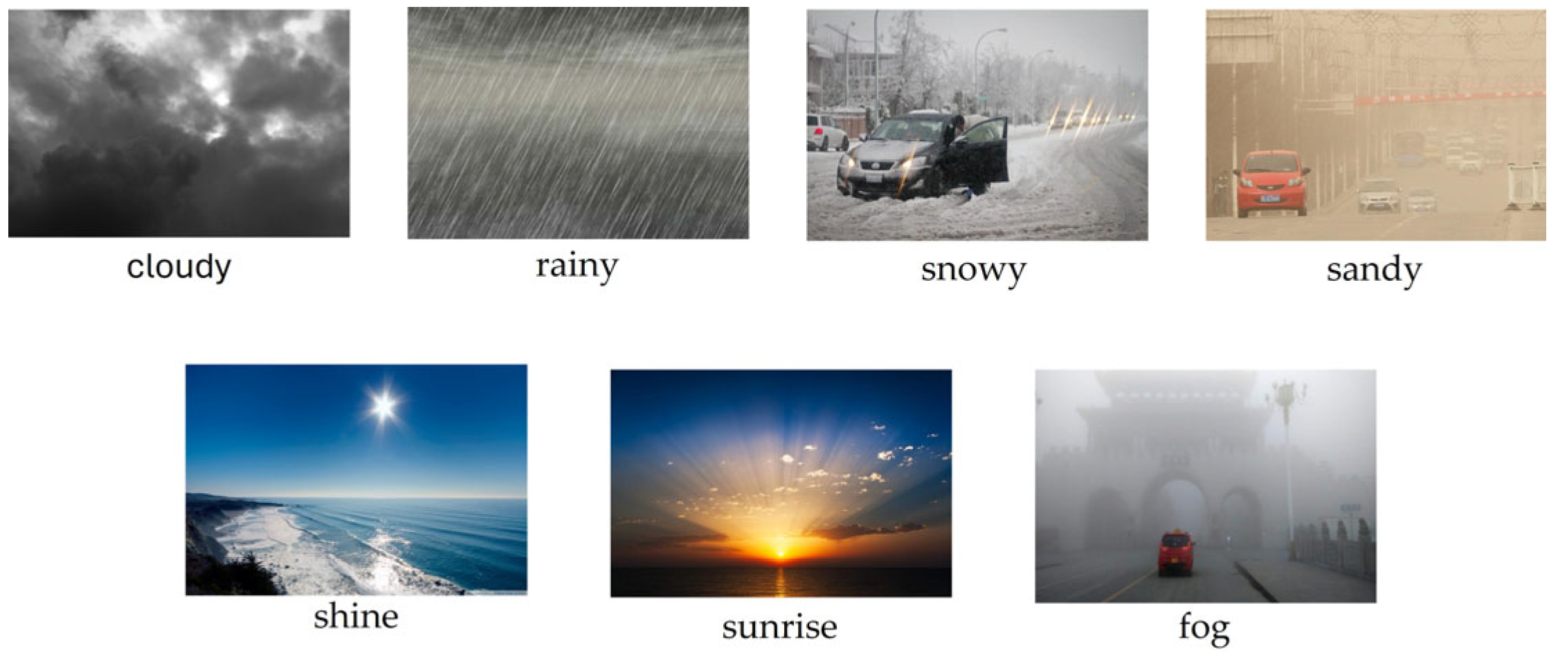
  • Original datasets: MCWRD2018 and DAWN2020 in seven categories (Figure 3).
  • Data augmentation: Original image, horizontally flipped image, and the original image cropped by 10% from each of the four sides.
  • Training and testing datasets: We split the augmenting dataset into the training (80%) and the testing datasets (20%). To ensure a fair evaluation, the two datasets’ contents are mutually exclusive.
  • Input resolution: 224 × 224.
  • Epoch: 300.
  • Batch size: 16.
  • Learning rate: 0.0001.
  • Loss function: CrossEntropyLoss.
  • Optimizer: Adam.
  • Language and machine library: Python [9] and PyTorch [10].
The experimental results are presented in Table 2. Among these models, the developed model achieved the best performance between accuracy and computational efficiency. It showed an accuracy of 98.37% with 0.3972 million parameters and 0.0955 GFLOPs. This proved its lightweight design and low computational costs. In contrast, EfficientNet-b0 showed a slightly higher accuracy of 98.61% but required over 10 times more parameters (4.0165 M) and significantly higher computational costs (0.4139 GFLOPs). ResNet-50 fell behind in accuracy (96.75%) and was much more resource-intensive, with 23.5224 million parameters and 4.1317 GFLOPs. SqueezeNet showed the lowest accuracy (73.82%), limiting its practical usability despite its relatively low parameter count and moderate GFLOPs. The results demonstrated that the model of this study outperformed others in terms of accuracy-to-efficiency ratio, making it superior for real-time embedded applications where resources are limited.

5. Conclusions and Future Work

We developed a lightweight and efficient weather perception model that enhanced the adaptability of autonomous driving systems under diverse environmental conditions. By considering an additional weather class and utilizing a modular and multi-branch neural architecture, the model demonstrated better classification accuracy while maintaining a significantly smaller parameter size and computational cost. The results confirmed its superiority for deployment in resource-constrained or real-time embedded systems. It is necessary to expand the weather classes to more region-specific phenomena or incorporate video sequences to improve classification robustness under rapidly changing conditions. Both ensure more intelligent autonomous driving systems.

Author Contributions

Conceptualization, T.-Y.T. and C.-C.C.; methodology, P.-T.W., T.-Y.T. and C.-C.C.; software, P.-T.W. and T.-Y.T.; validation, P.-T.W., T.-Y.T. and C.-C.C.; writing—original draft preparation, P.-T.W. and C.-C.C.; writing—review and editing, C.-C.C. All authors have read and agreed to the published version of the manuscript.

Funding

This work was supported by the National Science and Technology Council, Taiwan, under Grant 112-2221-E-035-062-MY3.

Institutional Review Board Statement

Not applicable.

Informed Consent Statement

Not applicable.

Data Availability Statement

Data will be made available on reasonable request.

Conflicts of Interest

The authors declare no conflicts of interest.

References

  1. Al-Haija, Q.A.; Gharaibeh, M.; Odeh, A. Detection in Adverse Weather Conditions for Autonomous Vehicles via Deep Learning. AI 2022, 3, 303–317. [Google Scholar] [CrossRef]
  2. Multi-Class Weather Dataset for Image Classification—Mendeley Data. Available online: https://data.mendeley.com/datasets/4drtyfjtfy/1 (accessed on 8 April 2025).
  3. DAWN—Mendeley Data. Available online: https://data.mendeley.com/datasets/766ygrbt8y/3 (accessed on 8 April 2025).
  4. Ooi, Y.-M.; Chang, C.-C.; Su, Y.-M.; Chang, C.-M. Vision-Based UAV Localization on Various Viewpoints. IEEE Access 2025, 13, 38317–38324. [Google Scholar] [CrossRef]
  5. Iandola, F.N.; Han, S.; Moskewicz, M.W.; Ashraf, K.; Dally, W.J.; Keutzer, K. SqueezeNet: AlexNet-level accuracy with 50x fewer parameters and <0.5MB model size. arXiv 2016, arXiv:1602.07360. [Google Scholar]
  6. He, K.; Zhang, X.; Ren, S.; Sun, J. Deep Residual Learning for Image Recognition. arXiv 2015, arXiv:1512.03385. [Google Scholar] [CrossRef]
  7. Tan, M.; Le, Q.V. EfficientNet: Rethinking Model Scaling for Convolutional Neural Networks. arXiv 2020, arXiv:1905.11946. [Google Scholar] [CrossRef]
  8. Hwang, K. Cloud Computing for Machine Learning and Cognitive Applications; The MIT Press: Cambridge, MA, USA, 2017. [Google Scholar]
  9. Welcome to Python.org. Available online: https://www.python.org/ (accessed on 8 April 2025).
  10. PyTorch. Available online: https://pytorch.org/ (accessed on 8 April 2025).
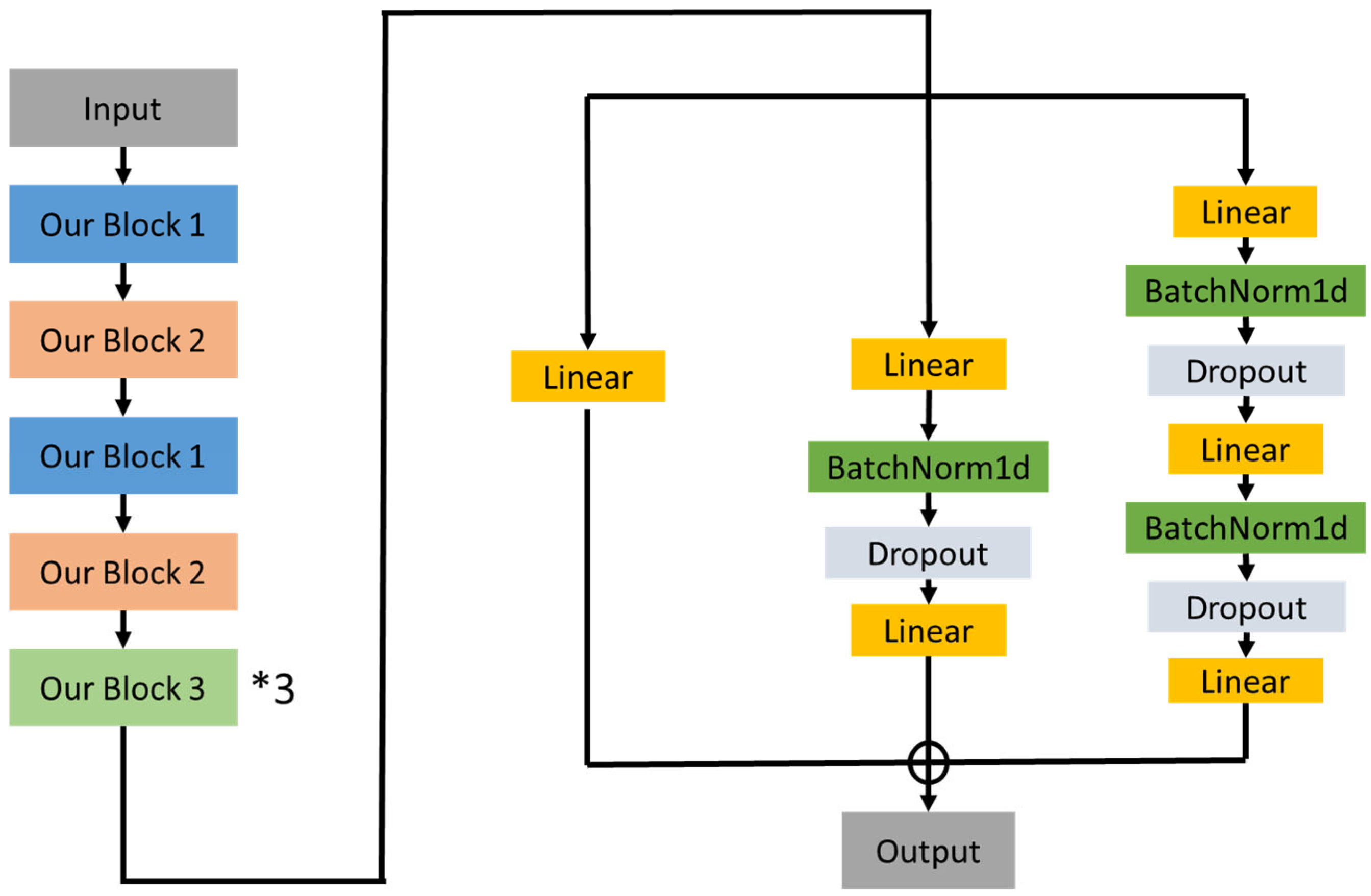
Figure 1. Architecture of neural network of developed model in this study. * indicates repetition.
Engproc 108 00018 g001
Figure 2. Custom blocks: (a) block 1, (b) block 2, and (c) block 3. * indicates repetition.
Engproc 108 00018 g002
Figure 3. Examples of seven weather categories.
Engproc 108 00018 g003
Table 1. Experimental procedure.
Procedures: Training and testing procedures in our weather perception approach.
input:
(01) data: a combination of MCWRD2018 and DAWN2020;
variables:
(02) augmenting-data: a dataset;
(03) training-data: a dataset;
(04) testing-data: a dataset;
(05) model: our machine learning model;
(06) benchmarks: the models used in [1];
initial phase:
(07) augmenting-dataaugment data;
(08) training-datasplit augmenting-data into 80% for training;
(09) testing-datasplit augmenting-data into 20% for testing;
training phase:
(10) train model via training-data;
(11) train benchmarks via training-data;
evaluating phase:
(11) evaluate model via testing-data;
(12) evaluate benchmarks via testing-data.
Table 2. Comparison of experimental models.
ModelEpochAccuracyParameter (Million)GFLOPs
Developed model29098.370.39720.0955
EfficientNet-b028298.614.01650.4139
ResNet-5029796.7523.52244.1317
SqueezeNet14073.821.25540.8191
Disclaimer/Publisher’s Note: The statements, opinions and data contained in all publications are solely those of the individual author(s) and contributor(s) and not of MDPI and/or the editor(s). MDPI and/or the editor(s) disclaim responsibility for any injury to people or property resulting from any ideas, methods, instructions or products referred to in the content.