1. Introduction
In recent years, renewable energy sources have gained significant attention as sustainable alternatives, with geothermal power generation being one of the most promising forms [
1]. Unlike solar or wind power, geothermal power harnesses high-temperature water and steam from deep underground, making it less susceptible to weather conditions and a viable baseload power source [
2,
3]. However, prolonged operation of geothermal wells often leads to a gradual decline in steam production due to factors such as reservoir pressure depletion, flow path blockage, and scale deposition [
4,
5,
6,
7]. These factors contribute to reduced power generation efficiency, increased risks of unplanned shutdowns, and higher operational costs.
Despite advancements in geothermal technology, the underlying physical and chemical processes governing anomalies in geothermal reservoirs remain partially understood, making it difficult to accurately identify the causes of steam production fluctuations [
8,
9]. As a result, planned shutdowns and appropriate maintenance strategies are crucial for effective geothermal well management [
10]. Traditionally, maintenance schedules have been determined based on periodic inspections and empirical analysis of operational data. However, failure to detect early signs of anomalies can lead to sudden production drops and equipment failures, significantly impairing power generation efficiency. Conversely, excessive maintenance can impose unnecessary costs and result in production losses due to operational downtime. Thus, there is a strong demand for objective and automated anomaly detection techniques [
11].
To address these challenges, this study proposes an anomaly detection system for geothermal steam production time-series data using Singular Spectrum Analysis (SSA). In particular, we focus on the largest singular value (i.e., the first principal component in SSA) and compute the corresponding left singular vector for the current time window. By comparing it with the left singular vector from past data, we derive an anomaly score that reflects how much the present time-series segment diverges from historical patterns. A data point is classified as anomalous when this score exceeds a predefined threshold. This approach enables early detection of anomalies that conventional methods may overlook, supporting more accurate operational decisions.
To evaluate the effectiveness of the proposed method, we conduct experiments using real geothermal power plant data and assess its anomaly detection performance. Furthermore, we analyze the impact of different threshold settings and explore the feasibility of well-specific adaptive anomaly detection. Specifically, we compare two threshold-setting approaches: (1) a unified threshold for all wells, optimized for maximum F1 score, and (2) individual thresholds for each well, optimized separately to maximize F1 score. This paper presents the experimental results, discusses the effectiveness of the proposed method, provides guidelines for optimal threshold selection, and highlights future research directions.
2. Method
Figure 1 illustrates the workflow of the anomaly detection method employed in this study. First, the collected steam production data undergoes preprocessing. During this step, a Butterworth low-pass filter is applied for noise removal and smoothing. This filtering process reduces the influence of unnecessary high-frequency components, enabling more precise anomaly detection.
Next, SSA is applied to decompose the time-series data using SVD. The singular values extracted from SSA serve as anomaly scores, which are used to detect abnormalities. The anomaly detection threshold is determined by optimizing the F1 score using training data.
Finally, the optimized threshold is applied to the test dataset to evaluate the performance of anomaly detection. The evaluation metrics include the Receiver Operating Characteristic (ROC) curve and the Precision–Recall (PR) curve, which quantitatively assess the accuracy of the detection model.
The following subsections provide a detailed explanation of each process.
2.1. Data Collection
This study utilizes steam production data from nine geothermal wells. The dataset consists of time-series records sampled at 5-min intervals over 14 years (2007–2021). Since each geothermal well exhibits unique production characteristics, the data does not follow a single pattern but instead demonstrates various fluctuations. These fluctuations are influenced by well conditions and operational factors, sometimes resulting in abrupt changes in steam production. This study aims to identify such fluctuations as anomalies and develop an anomaly detection model for their classification and evaluation.
The data collection process involved the following steps:
2.2. Smoothing and Noise Reduction Using Butterworth Filter
In singular spectrum analysis, if the time-series data contains noise, there is a risk of mistakenly identifying unintended noise as an anomaly. Therefore, in this study, a Butterworth low-pass filter was applied as a preprocessing step to the steam production data to remove high-frequency noise and smooth the data [
12]. The Butterworth filter is widely used for noise reduction and signal smoothing in various applications. It is particularly suitable for this task because it provides a maximally flat frequency response in the transition band, effectively suppressing high-frequency components while preserving the overall trend of the data.
In geothermal power generation, noise can arise due to measurement errors, seismic activity, and external environmental influences. When applying butterworth filtering, excessively narrowing the transition band may result in the loss of actual steam production variations. Therefore, an appropriate setting of the transition band is crucial.
This study set the transition band within a frequency range of 7 to 11 oscillations per day. This range was determined to allow a certain level of noise while effectively eliminating high-frequency components.
2.3. SSA for Anomaly Detection
In this study, SSA was applied to analyze the time-series data of steam production and detect anomalies. SSA is a powerful non-parametric technique that decomposes time-series data into interpretable components such as trends, periodicity, and noise [
13]. The basic steps of SSA are outlined below.
- 1.
Embedding
The time-series data
is used to construct a Trajectory Matrix as follows (
1):
In Equation (
1),
w represents the number of data points extracted from the time series, corresponding to the number of matrix rows, and
K denotes the number of shifts in the time series, corresponding to the number of matrix columns. This study used
w = 12 and
K = 12 to capture one hour of data. Additionally, to account for past data, we constructed a similar Trajectory Matrix (
2) by going back
L = 24 steps (two hours). These parameters were chosen to capture abrupt fluctuations in steam production while avoiding excessive redundancy.
- 2.
SVD
SVD is applied to the constructed matrix
, decomposing it as follows (
3):
where
U is the left singular vector matrix,
is the diagonal matrix of singular values, and
V is the right singular vector matrix.
Similarly, SVD is applied to
, the past trajectory matrix, as shown in (
4):
- 3.
Computation of Anomaly Score
To perform anomaly detection based on SSA, we evaluate the norm of the first-column component
derived from the left singular vectors of the current data
and the first-column component
derived from the left singular vectors of the past data
. Because this first-column component corresponds to the largest singular value, it allows for a low-cost extraction of a vector with high singularity. We then define the anomaly score according to Equation (
5).
Here, represents the norm between the singular vectors of the current and past data. Since these vectors belong to an orthonormal basis, the inequality holds. Consequently, the anomaly score is constrained within the range , where a higher value indicates a greater degree of anomaly.
2.4. Non-Maximum Suppression
In this study, Non-Maximum Suppression (NMS) is applied to the time series of anomaly scores computed by SSA to reduce false detections. NMS is traditionally used in computer vision to eliminate redundant detections in object detection tasks. However, this study adapted it for time-series data to aggregate closely occurring peaks and treat them as a single significant anomaly.
Procedure
- 1.
Set the window size
A fixed-width window is defined along the time axis.
- 2.
Select the maximum value within each window
Only the maximum anomaly score within each window is retained, while all other values are suppressed.
- 3.
Reconstruct the anomaly scores
The window is iteratively shifted across the entire time series, ensuring that only the highest anomaly score remains within each window.
By consolidating consecutive high anomaly scores into a single anomaly event, this method enhances interpretability and facilitates alarm management in operational settings. Additionally, in the final anomaly score plot, peaks become more structured and visually distinct, allowing operators to intuitively grasp the timing of major anomalies.
2.5. Threshold Optimization and Alarm Setting
To detect anomalies using the anomaly score derived from SSA, it is essential to establish an appropriate threshold. The threshold is determined by considering the distribution of anomaly scores and optimizing it to maximize classification accuracy between normal and anomalous states. This section describes the threshold selection method.
In anomaly detection, achieving a high recall is crucial to avoid missing anomalies, while excessive anomaly detection can lead to an increased false alarm rate. Therefore, precision must also be considered. In this study, the threshold was chosen to maximize the F1 score on the training dataset.
One key advantage of the F1 score is that it balances precision and recall, ensuring an optimal trade-off between anomaly detection accuracy and false alarms. The threshold that maximizes the F1 score was selected for implementation.
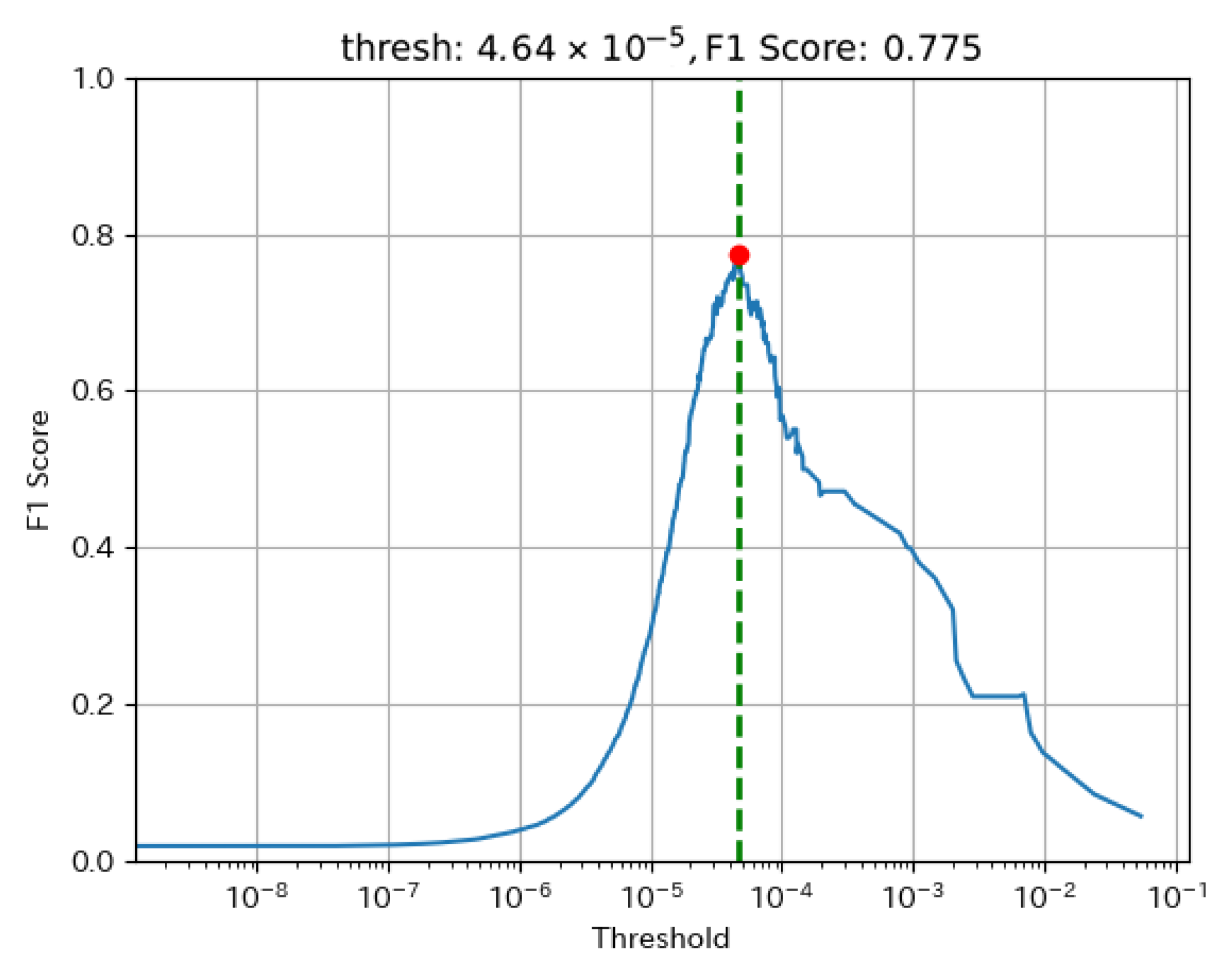
Figure 2 illustrates the relationship between the threshold and the F1 score for a representative well. The red point represents the selected threshold, corresponding to the highest F1 score on the training dataset.
2.6. Evaluation
To assess the performance of the proposed anomaly detection method, the optimized threshold was applied to the validation dataset. The evaluation was conducted using two standard performance metrics: the ROC and PR curves.
The ROC curve illustrates the relationship between the TPR and the FPR across different threshold values. This allows for a visual assessment of the optimal threshold for anomaly detection.
Additionally, the Area Under the Curve (AUC) of the ROC curve is widely used as a quantitative measure of model performance. AUC values closer to 1.0 indicate better performance, while values near 0.5 suggest that the model performs no better than random classification.
The PR curve evaluates model performance by considering Precision (the proportion of predicted anomalies that are actual anomalies) and Recall (the proportion of actual anomalies that are correctly identified).
The PR curve is particularly effective in scenarios where anomalies constitute a small fraction of the dataset, as it directly measures how many detected anomalies are correct and how many actual anomalies are successfully identified, making it less affected by class imbalance.
3. Results
This section presents the results of anomaly detection using the proposed method. The evaluation was conducted under two different thresholding approaches: (1) a unified threshold optimized for all wells and (2) individual thresholds optimized separately for each well. The performance metrics obtained for each case are summarized in
Table 1 and
Table 2. Additionally, visualized anomaly detection results and a comparison of ROC and PR curves are reported.
3.1. Comparison of Performance Metrics
Table 1 presents the performance metrics obtained using a single unified threshold for all wells. The threshold value was determined through optimization to maximize the F1 score. The table includes values for F1 score, Precision, Recall, TPR, and FPR.
Table 2 presents the performance metrics when optimizing individual thresholds for each well. The results indicate substantial variations in the optimal threshold values, as well as in the F1 score, Precision, and Recall, depending on the well.
3.2. Visualization of Anomaly Detection Results
This subsection presents visualized examples of the anomaly detection results.
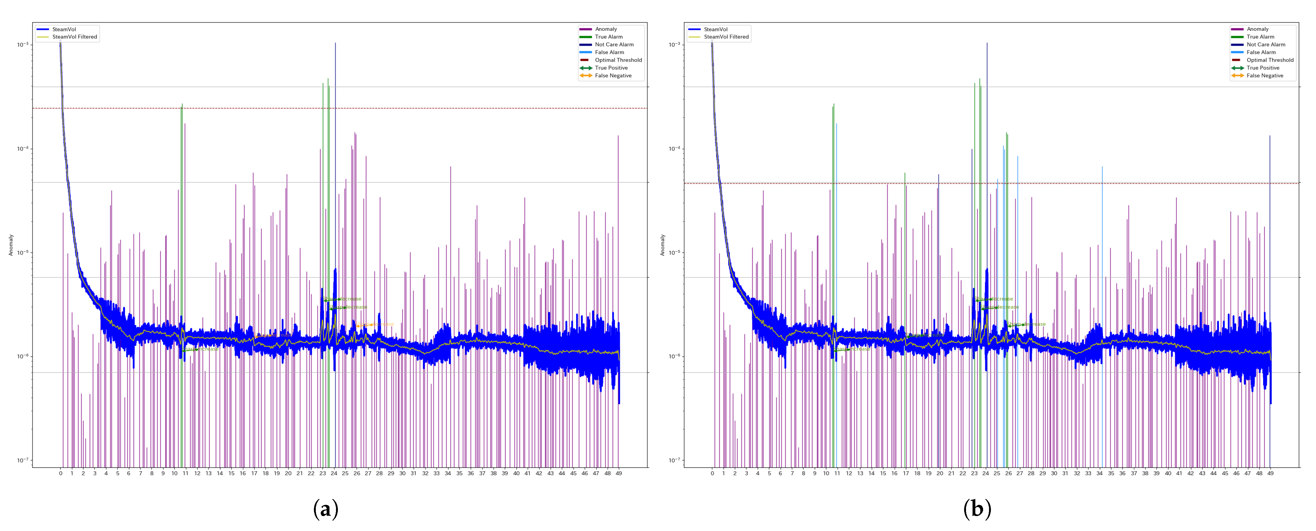
Figure 3 illustrates the results for a specific segment of Well 4 (denoted as W4), comparing the outcomes obtained using a unified threshold and individual thresholds.
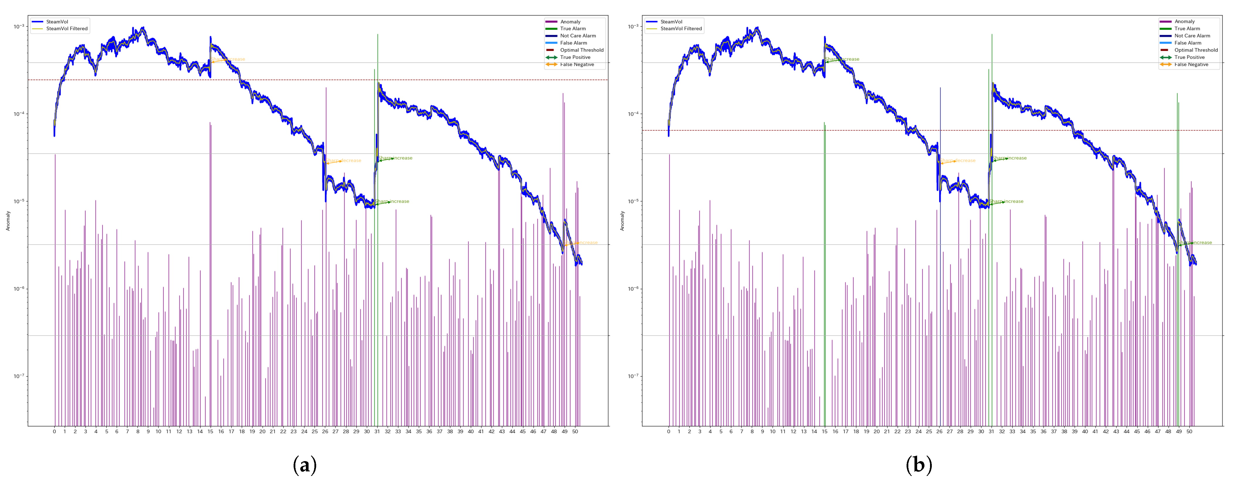
The blue and yellow lines represent the original steam production data and the filtered series, respectively. The green and orange arrows indicate manually assigned anomaly labels, distinguishing between True Positives (TPs) and False Negatives (FNs).
The bar graph represents the anomaly scores computed using SSA. Purple bars indicate True Negatives (TNs). Green bars indicate True Positives (TPs). Light blue bars indicate False Positives (FPs). Dark blue bars represent detected anomalies that do not correspond to abrupt changes in the manually assigned labels.
The dashed line represents the threshold used for classification, and any anomaly score exceeding this threshold is classified as an anomaly.
Comparing the
a (unified threshold) and the
b (individual threshold) in
Figure 3, the individual threshold is set at a lower value, leading to an increase in false positives, which in turn reduces the F1 score. Similarly,
Figure 4 illustrates the results for another segment of Well 1 (denoted as W1). In this case, the individual threshold reduces the number of false negatives (FNs), thereby improving the F1 score.
3.3. ROC and PR Curves
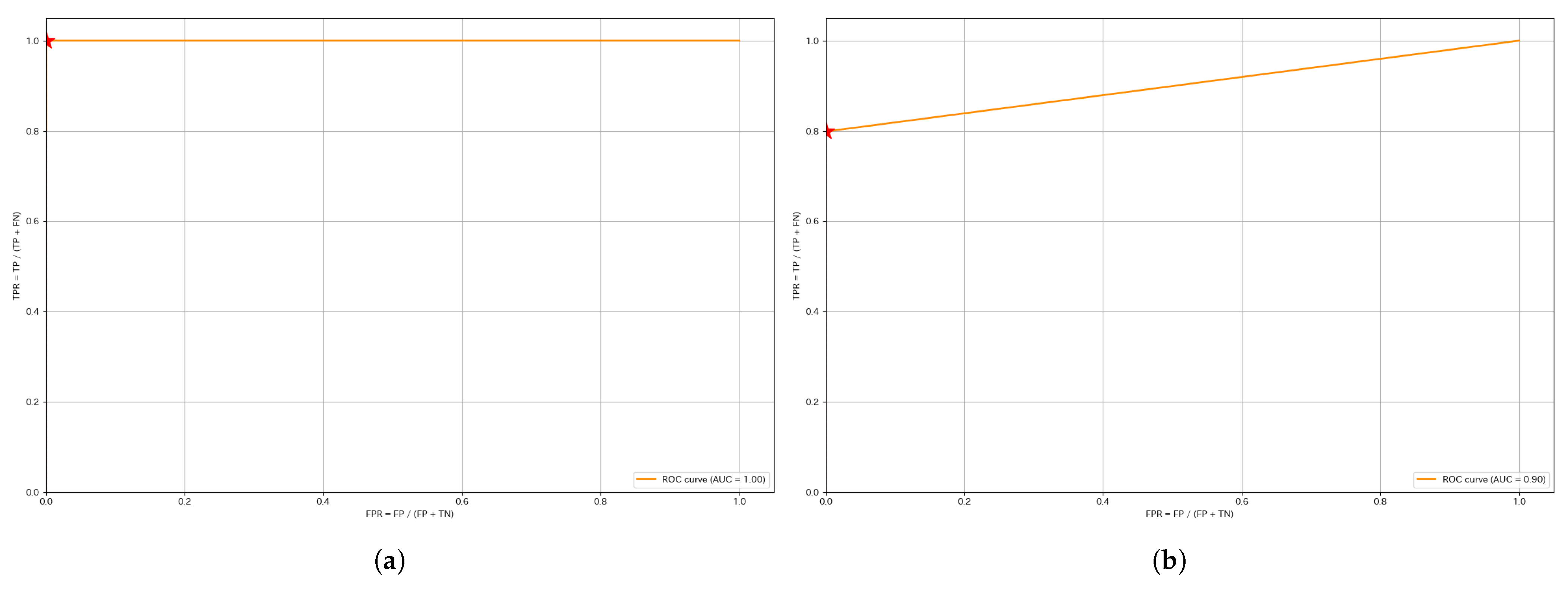
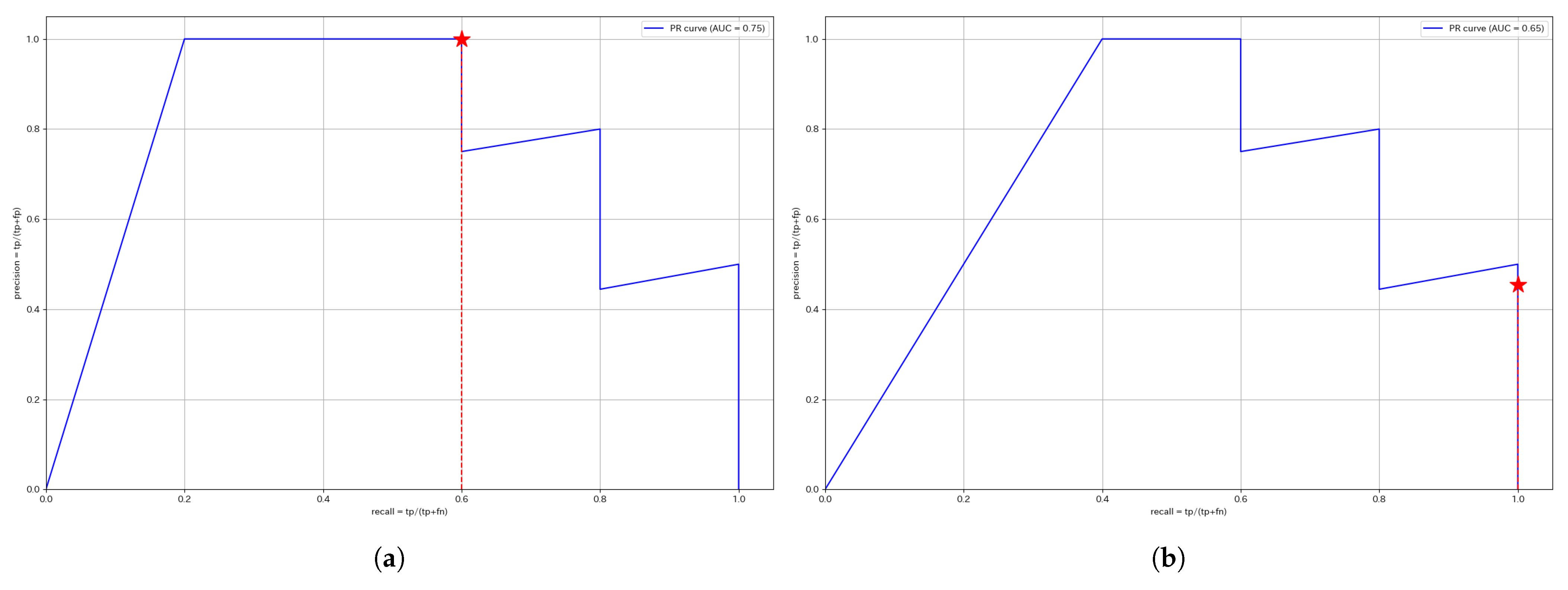
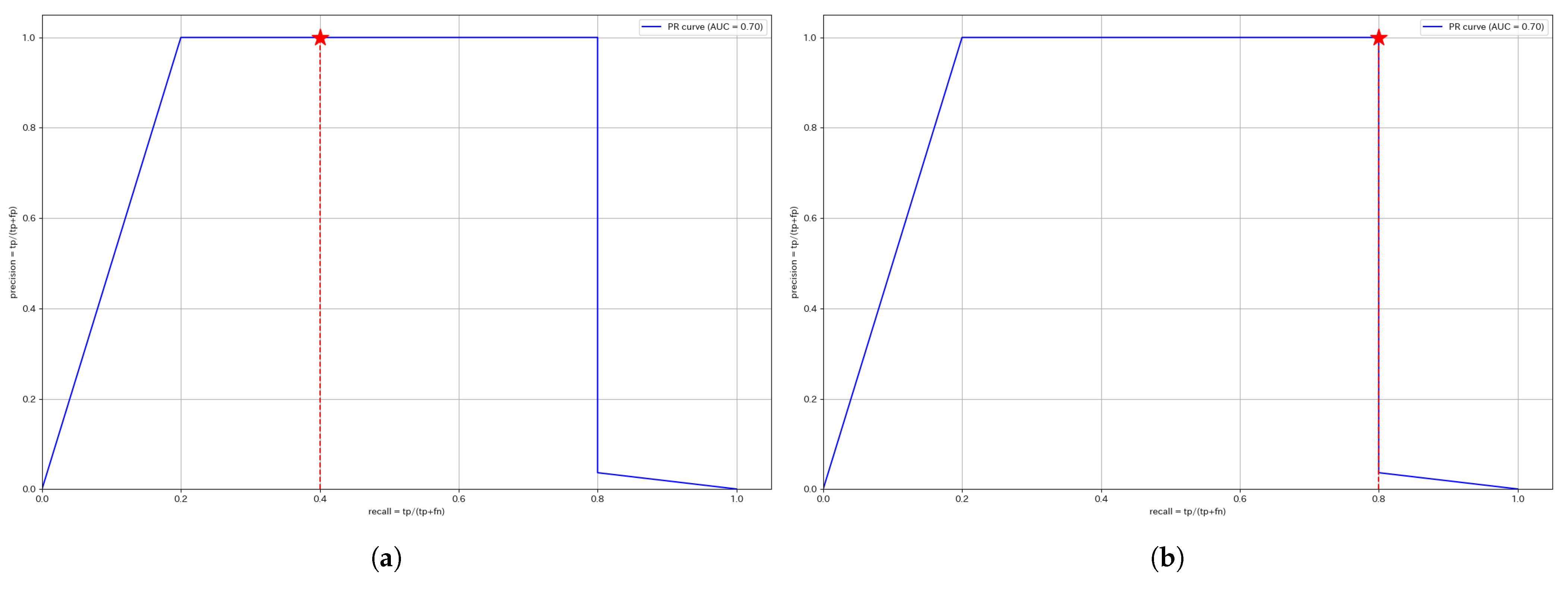
This section presents the ROC and PR curves. Since the anomaly score calculation is identical, the curves for the same segment remain unchanged regardless of whether a unified threshold or individual thresholds are used. The red stars plotted in each figure indicate the Precision and Recall values at the optimized threshold determined using the training data.
Figure 5 shows the ROC curves for W4 and W1. Most ROC curves, including those not shown here, exhibit a shape approaching the upper left corner, with AUC values close to 1. This suggests that the model is able to distinguish anomalies from normal data with relatively high accuracy. However, it also reflects the class imbalance in the dataset. Since the dataset is imbalanced, such results are expected.
Figure 6 presents the PR curves for W4, while
Figure 7 displays the PR curves for W1. The F1 score is the harmonic mean of Precision and Recall, meaning that a curve closer to the upper right corner indicates a higher F1 score. Therefore, segments, where the curve approaches the upper right corner, suggest that anomalies are effectively captured using the anomaly score.
For W4, the unified threshold achieves a Precision of 1, while the individual threshold achieves a Recall of 1. Since the Recall of the unified threshold is higher than the Precision of the individual threshold, the F1 score is higher for the unified threshold, making it the better approach for W4.
For W1, both thresholds achieve a Precision of 1. However, since the individual threshold achieves a higher Recall, the F1 score is higher for the individual threshold, making it the better approach for W1.
These results indicate that optimizing thresholds for individual wells does not always guarantee improved accuracy. It is crucial to consider the operational conditions and characteristics of each well when selecting an appropriate threshold.
4. Discussion
This study applied SSA to geothermal well steam production data and validated its effectiveness for anomaly detection. Based on the results presented in the Results section, the following insights were obtained:
4.1. Threshold Selection and Adaptation to Well Characteristics
This study examined two approaches: a unified threshold for all wells and individual thresholds for each well. Both methods have their own advantages and challenges.
For the unified threshold, a single threshold is applied across all wells, increasing the amount of data and capturing average characteristics. However, in some wells, this approach leads to a higher rate of false positives or false negatives, resulting in a lower F1 score.
For the individual threshold, thresholds are optimized for each well, allowing for greater flexibility in wells with distinct characteristics. However, when the behavior of a well deviates from past patterns, the effectiveness of this approach may be reduced.
These results indicate that optimizing thresholds for individual wells does not always guarantee improved accuracy. Instead, a balanced threshold design tailored to each well’s characteristics is necessary.
4.2. Insights from ROC and PR Curves
The ROC curves confirm that the dataset is imbalanced, with anomalies being significantly fewer than normal data. The PR curves further demonstrate how Precision and Recall trade-offs vary based on the selected threshold. Particularly in cases where the class imbalance is severe, PR curves allow for a more accurate assessment of false positive (FP) and false negative (FN) risks.
For instance, in W1, the AUC of the ROC curve did not reach 1, suggesting that some anomalies exhibit lower anomaly scores, leading to potential misclassifications. This finding indicates the need for further refinement of the anomaly score calculation method.
4.3. Operational Challenges in Anomaly Detection
In practical geothermal power plant operations, this study primarily focused on detecting sudden changes in steam production. However, future research should consider other types of anomalies, such as reservoir characteristics or scale deposition. Effective classification and differentiation of these anomalies remain a key challenge.
From an operational standpoint, early anomaly detection can help prevent unscheduled shutdowns, which may lead to significant losses in power generation and increased maintenance costs. For instance, detecting anomalies even 1–2 days earlier could translate into substantial cost savings, depending on the plant’s capacity and the responsiveness of maintenance teams.
Additionally, SSA primarily focuses on trend analysis of production volumes. Integrating SSA with geological modeling, pressure monitoring, and temperature observations could enable more precise anomaly detection and root cause analysis.
4.4. Limitations and Future Work
Although SSA effectively decomposes time-series data into interpretable components, it has limitations. The choice of window length and embedding dimension strongly influences the decomposition, and inappropriate settings can cause either over-smoothing or sensitivity to noise. Moreover, SSA assumes stationarity within each window, which may not hold in rapidly changing geothermal environments. Therefore, additional verification is required to evaluate the generalizability of the proposed method to other geothermal sites and wells.
Future research should focus on the following:
Refining anomaly classification: Identifying different anomaly types beyond sudden production drops.
Cost-aware optimization: Incorporating shutdown costs, repair costs, and other economic factors to enhance operational decision-making.
Extended threshold optimization: Expanding the threshold optimization approach to include well-specific error estimates and geological parameters for a more comprehensive anomaly detection and adaptive control system.
Application to other domains: Leverage the general-purpose, noise-robust nature of the SSA-based framework to apply it to other industrial time-series data, such as photovoltaic output or wind turbine monitoring.
By addressing these areas, this research aims to contribute to the development of a practical and reliable anomaly detection system for geothermal power plant operations.
5. Conclusions
This study applied SSA to geothermal well steam production data and proposed an anomaly detection method based on singular values. The effectiveness of the proposed approach was evaluated through comparative analysis.
The approach of setting individual thresholds for each well has the potential to capture well-specific characteristics and improve F1 score. However, it also carries the risk of overfitting due to insufficient training data. Conversely, using a unified threshold across all wells allows for a larger dataset but may fail to adequately address well-specific anomalies.
By utilizing both ROC and PR curves, it was confirmed that threshold selection significantly affects model performance. In particular, for datasets with severe class imbalance, PR curves and F1 score evaluations proved to be more effective for assessing anomaly detection performance.
These findings suggest that SSA-based anomaly detection is a valuable tool for supporting shutdown decisions in geothermal power plants. Future research should focus on refining anomaly classification to account for different types of anomalies, incorporating economic factors into a comprehensive optimization framework, and integrating geological parameters to improve anomaly detection accuracy. Addressing these aspects is expected to contribute to the development of a more practical and reliable anomaly detection system for geothermal well operations.
Furthermore, given the non-parametric nature and noise robustness of the proposed framework, its applicability is not limited to geothermal settings. Although this study focused on geothermal steam production, the SSA-based anomaly detection method could also be extended to other industrial time-series applications such as photovoltaic output monitoring and wind turbine diagnostics.
Author Contributions
K.A.: Conceptualization, methodology, investigation, writing—original draft preparation. Y.H.: Conceptualization, writing—review and editing, supervision. All authors have read and agreed to the published version of the manuscript.
Funding
This work was supported by The New Energy and Industrial Technology Development Organization (NEDO) JPNP21001.
Institutional Review Board Statement
Not applicable.
Informed Consent Statement
Not applicable.
Data Availability Statement
The data used in this study were collected by Okuaizu Geothermal Co., Ltd. and are currently available only within the scope of this research project. Therefore, the data cannot be shared with third parties.
Acknowledgments
The authors would like to thank Oku-Aizu Geothermal Co., Ltd. for providing the time-series data and expert annotations used in this study.
Conflicts of Interest
The authors declare no conflicts of interest.
References
- Rakhmatov, A.; Primov, O.; Mamadaliyev, M.; Tòrayev, S.; Xudoynazarov, U.; Xaydarov, S.; Ulugmurodov, E.; Razzoqov, I. Advancements in renewable energy sources (solar and geothermal): A brief review. E3S Web Conf. 2024, 497, 01009. [Google Scholar] [CrossRef]
- Adams, C.A.; Auld, A.M.; Gluyas, J.G.; Hogg, S. Geothermal energy–The global opportunity. Proc. Inst. Mech. Eng. Part A J. Power Energy 2015, 229, 747–754. [Google Scholar] [CrossRef]
- Basosi, R.; Bonciani, R.; Frosali, D.; Manfrida, G.; Parisi, M.L.; Sansone, F. Life cycle analysis of a geothermal power plant: Comparison of the environmental performance with other renewable energy systems. Sustainability 2020, 12, 2786. [Google Scholar] [CrossRef]
- Baymatov, S.H.; Kambarov, M.; Berdimurodov, A.; Tulyaganov, Z.; Muminov, A. Employing Geothermal Energy: The Earth’s Thermal Gradient as a Viable Energy Source. E3S Web Conf. 2023, 449, 06008. [Google Scholar] [CrossRef]
- Duplyakin, D.; Beckers, K.F.; Siler, D.L.; Martin, M.J.; Johnston, H.E. Modeling subsurface performance of a geothermal reservoir using machine learning. Energies 2022, 15, 967. [Google Scholar] [CrossRef]
- Longval, R.; Meirbekova, R.; Fisher, J.; Maignot, A. An Overview of Silica Scaling Reduction Technologies in the Geothermal Market. Energies 2024, 17, 4825. [Google Scholar] [CrossRef]
- Fanicchia, F.; Karlsdottir, S.N. Research and Development on Coatings and Paints for Geothermal Environments: A Review. Adv. Mater. Technol. 2023, 8, 2202031. [Google Scholar] [CrossRef]
- Guillou-Frottier, L.; Duwiquet, H.; Launay, G.; Taillefer, A.; Roche, V.; Link, G. On the morphology and amplitude of 2D and 3D thermal anomalies induced by buoyancy-driven flow within and around fault zones. Solid Earth 2020, 11, 1571–1595. [Google Scholar] [CrossRef]
- Barragán, R.M.; Arellano, V.M.; Nieva, D. Analysis of Geochemical and Production Well Monitoring Data—A Tool to Study the Response of Geothermal Reservoirs to Exploitation. In Advances in Geothermal Energy; IntechOpen: London, UK, 2016. [Google Scholar]
- Buster, G.; Siratovich, P.; Taverna, N.; Rossol, M.; Weers, J.; Blair, A.; Huggins, J.; Siega, C.; Mannington, W.; Urgel, A.; et al. A new modeling framework for geothermal operational optimization with machine learning (Gooml). Energies 2021, 14, 6852. [Google Scholar] [CrossRef]
- Liu, Y.; Ling, W.; Young, R.; Zia, J.; Cladouhos, T.T.; Jafarpour, B. Latent-space dynamics for prediction and fault detection in geothermal power plant operations. Energies 2022, 15, 2555. [Google Scholar] [CrossRef]
- Wang, B. Signal Processing Based on Butterworth Filter: Properties, Design, and Applications. Highlights Sci. Eng. Technol. 2024, 97, 72–77. [Google Scholar] [CrossRef]
- Espinosa, F.; Bartolomé, A.B.; Hernández, P.V.; Rodriguez-Sanchez, M. Contribution of singular spectral analysis to forecasting and anomalies detection of indoors air quality. Sensors 2022, 22, 3054. [Google Scholar] [CrossRef]
| Disclaimer/Publisher’s Note: The statements, opinions and data contained in all publications are solely those of the individual author(s) and contributor(s) and not of MDPI and/or the editor(s). MDPI and/or the editor(s) disclaim responsibility for any injury to people or property resulting from any ideas, methods, instructions or products referred to in the content. |
© 2025 by the authors. Licensee MDPI, Basel, Switzerland. This article is an open access article distributed under the terms and conditions of the Creative Commons Attribution (CC BY) license (https://creativecommons.org/licenses/by/4.0/).

