Abstract
In the contemporary era, the pursuit of precise predictions based on datasets is predominantly motivated by the science of computer systems. Therefore, this study attempts to further enhance prediction efforts. A city-wide electricity consumption dataset, which includes temporal and environmental characteristics, is analyzed. This dataset is subjected to rigorous preprocessing to extract relevant characteristics. A wide range of machine learning models, such as XGBoost and Python’s Scikit, are used to build prediction models. These models are then rigorously trained and tuned using sophisticated optimization techniques for optimal performance. Finally, the evaluation of their efficiency, interpretability, and computational efficiency is derived. Furthermore, programming techniques are investigated, and new structures and learning methods elucidate intricate patterns and relationships in the data. This approach facilitates a more comprehensive understanding of the pivotal factors influencing electrical consumption trends and enables the identification of the most suitable methodologies for specific prediction tasks. In conclusion, the present study contributes by utilizing the knowledge gained from previous research for the advancement of predictive analysis. The findings have the potential to be useful in decision-making processes, optimizing resource allocation, and improving urban planning and management practices.
1. Introduction
In today’s world, there is a wealth of data concerning all areas of human and physical activity. This data is collected and stored for either prediction or improvement, which may involve, for example, saving resources, developing products and services, expanding markets, improving processes, security, protecting the environment, etc.
For this knowledge extraction, a variety of data mining methods and techniques have been developed and applied [1,2,3]. One of them is the use of machine learning [4].
The present work therefore hopes to contribute to the extension of the above methodology and also aims to improve previous prediction efforts with a different software approach [5,6].
Its aim is therefore to create a prediction model based on machine learning. This model was created using the Python programming interface because, through this environment, it was possible to access a large number of libraries related to data science [7]. The model was then trained using a combination of data collected from the area of the city of Kavala in Greece and related to environmental conditions such as temperature, humidity, rainfall, etc. [8]. The above were then combined with the variation in the city’s total electricity consumption, recorded at a frequency of half an hour, over the course of a year.
The created database, once properly cleaned and formatted, was fed into the model, which was then trained via supervised learning. Finally, the predictions generated were compared with the existing real values in order to evaluate the whole system through its results.
From the completion of the whole effort, the potential of the export of predictions and the analytical character of the method can be assessed. On the other hand, the need for a larger volume of data that will optimize the training and performance of the model is considered positive.
2. Materials and Methods
2.1. Model Training
Firstly, the algorithm’s code was created in a Python environment that includes libraries such as the Pandas and Numpy, etc. As the main library for the prediction model, XGBoost is employed for supervised learning, where the training data with multiple features xi is used to predict a target variable y. In this case, the prediction is expressed using the following equation:
where ŷ is the predicted value, (x1, x2, …, xn) are the input attributes, (w1, w2, …, wn) are the weights associated with each input attribute, and b is the bias [9,10,11]. Furthermore, the SKLearn metrics and Seaborn libraries were also implemented to visualize the charts from the database and to make a simpler comparison between the predictions and the actual data.
ŷ = w1x1 + w2x2 + … + wnxn + b,
Moreover, the initial data were subjected to prepossessing as shown in Figure 1, all the steps of the knowledge discovery process were followed.
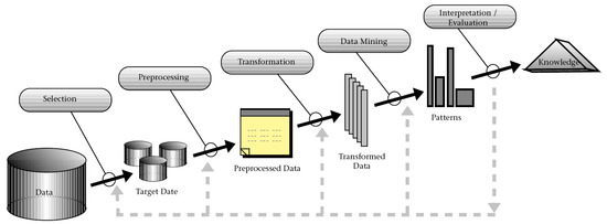
Figure 1.
The stages of the knowledge discovery process.
The above steps [12] will not be examined further as they are not the main purpose of the present work. It will only be mentioned that, during the Transformation stage, the format of some data was converted into numerical form in order to facilitate their processing by the machine learning algorithm.
As a next step, in order to obtain the prediction of electricity consumption, the constructed algorithm should initially be trained. For this purpose, the above data was provided to the model so that the learning process could be completed. The model was trained on labeled data (X_train, Y_train) where the input features (X_train) were paired with their corresponding target values (Y_train). The goal was to predict continuous numerical values (regression), which is a typical supervised learning task.
For the above purpose, the data was divided into two groups, as shown in Figure 2, where the dashed line in the month of September indicates the separation of the data.
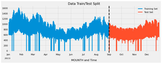
Figure 2.
Training and test data split.
Thus, up to the month of August, the data was used for training the algorithm and from September onwards was used for testing the prediction results obtained from the model.
2.2. Feature Creation
Feature Creation was then followed. This procedure creates time-based features from the DataFrame’s index and adds them as columns. It also includes existing weather and energy consumption features.
Every variable was then visualized in relation to the target variable, which is the electricity consumption. The following images are represented in the form of a Boxplot and provide information on the smallest and largest observations of the lower and upper quartile values (Q1 and Q3) and the median. From then it can be observed how much each variable influences energy consumption.
Figure 3 indicates the impact of the hours of the day compared to the electrical consumption. It can be observed that the peak use of electricity during the day is, in general, in the late evening hours between 18:00 and 21:00, and, in particular, the highest average consumption of the day is at 20:00, as it appears from the median. On the other hand, it can be observed that during the midnight hours, consumption drops significantly, with the lowest being at 04:00. These results seem obvious, but they prove that the process produces reasonable outcomes.
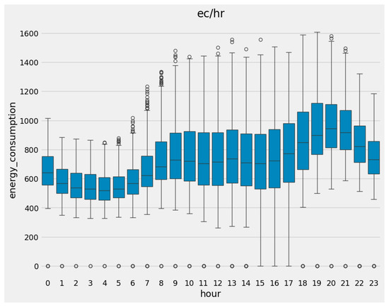
Figure 3.
Energy consumption during the day hours.
Furthermore, Figure 4 represents the effect that the days of the week have on electricity consumption. As can be observed, during the weekend days (Saturdays (5) and Sundays (6)), consumption is reduced. Moreover, it is derived that in the particular dataset, this variable has less impact on electricity consumption compared to the hour of the day.
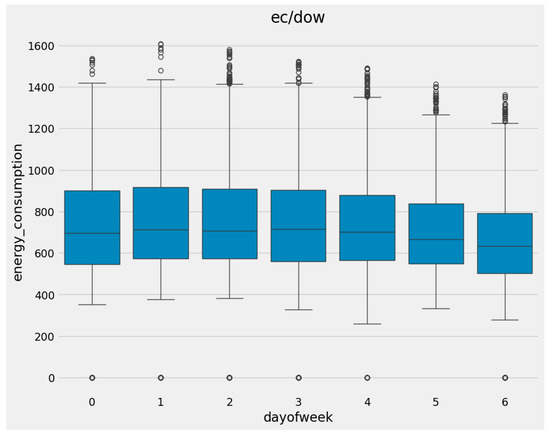
Figure 4.
Energy consumption per day of the week.
In addition, from Figure 5 it can be concluded that the winter season had a larger impact on the overall electricity consumption. This would suggest that people in the area would rather utilize electricity than other methods of heating to warm up in the colder months. Additionally, a slight increase in consumption in the summer months June and July can also be observed, which can be translated to electricity usage for cooling purposes.
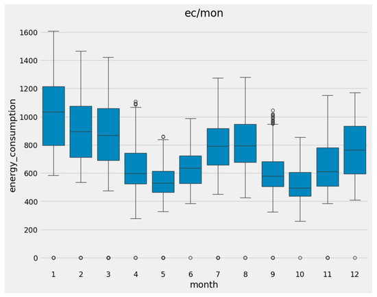
Figure 5.
Energy consumption per month.
The previous claims can also be confirmed by Figure 6, showing peaks in overall electricity consumption at temperatures between 5.6 and 9 degrees Celsius in winter and at about 25.5 degrees Celsius in summer time. Since consumption is therefore affected by temperature, it follows that part of the electrical energy is used to regulate it.
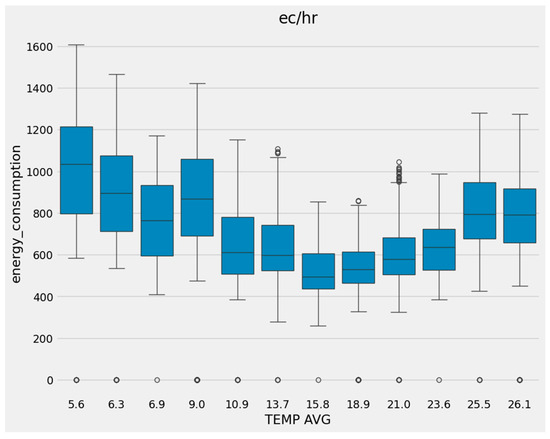
Figure 6.
Energy consumption compared to the average temperature.
As a result of all of the above, a summary diagram of the significance of the feature importance is obtained. As shown in Figure 7, it is obvious that in this specific database, the factor that most influences the consumption of electricity in the region is the hours of day.
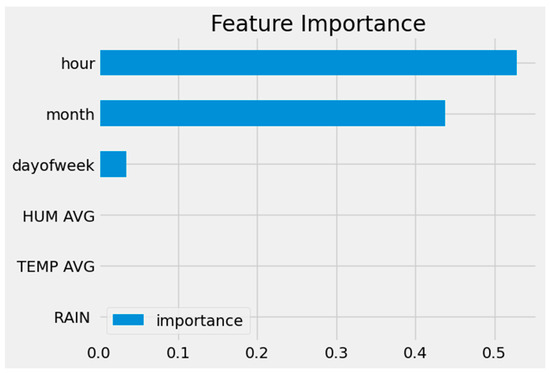
Figure 7.
Feature importance.
3. Model Creation
The following procedure is the creation of a model using the XGBoost algorithm [13]. Specifically, the boosted tree algorithm was implemented, with a selected number of 5000 trees.
For training, all the data was used, except for the consumption of electrical energy, which was set as a target. Subsequently, the regression from XGBoost was deployed from the library and the model was executed.
As a result of the above processes, the algorithm generated a prediction for the missing values of the test months (September, October, November, and December) based on the existing truth data.
This prediction is visualized in Figure 8.
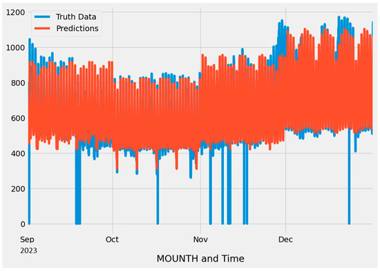
Figure 8.
Prediction for the test months.
As can easily be observed, the prediction is highly correlated with actual consumption. In addition, one of the advantages of this pattern is that it is modular, so it allows the data to be examined in greater detail. This gives the ability for research to be carried out at shorter intervals, even days or hours. In this case, Figure 9 shows the analysis for the first seven days of September 2023.
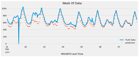
Figure 9.
General graph for the first week of September 2023.
The above figure illustrates in greater detail how the prediction follows actual consumption prices with considerable accuracy.
The results were subsequently evaluated using the Root Mean Square Error, with an evaluation metric of 42 R-squared. From this error, the best and worst predictions can be calculated, as shown in Table 1.

Table 1.
Relative errors.
As shown in Table 1, the lowest error was 14.94%, recorded on 24th October, and the highest was 19.6%, recorded on 15th September.
As a result of all the above procedures, Figure 10 is created. This is a record of the final prediction of electricity consumption for the whole year of 2024.
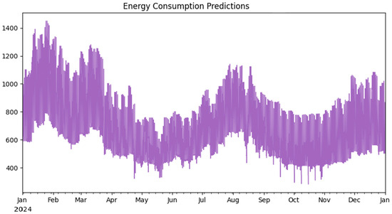
Figure 10.
Prediction for the year 2024.
The average value of the predictions is 704. On the other hand, the actual average value of the year 2024, based on the real recorded electrical consumption data, is 697. The real, existing values for consumption in 2024 are presented separately in the graph in Figure 11.
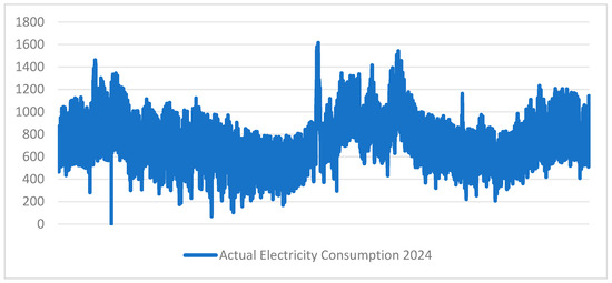
Figure 11.
Actual values for the year 2024.
As can be easily observed from the above two figures, there is an obvious similarity between the prediction (Figure 10) and the actual (Figure 11) consumption. That gives an estimated error of only 0.99%, which is relatively low and indicates that the developed machine learning algorithm has generated an output that can be considered reliable.
4. Conclusions
In this study, the XGBoost algorithm was employed to predict electricity consumption. The model was trained on real-world data, incorporating relevant features such as weather patterns, time-based factors, and environmental variables.
The findings indicate that XGBoost demonstrates promising potential in forecasting electricity consumption. The model achieved a relatively accurate prediction, with an RMSE of 42, and the percentage difference between the prediction and the actual average of electrical consumption was only 0.99%, suggesting its ability to capture complex patterns and relationships within the data.
However, further research and refinements are recommended to enhance the model’s predictive capabilities. This may involve exploring additional feature engineering techniques, optimizing hyperparameters, or incorporating more far-reaching external data sources to improve model robustness and accuracy.
Overall, the XGBoost model presents a valuable tool for stakeholders in the energy sector and beyond. As an outcome, accurate electricity consumption forecasting can aid in demand management, resource allocation, and grid stability, contributing to a more efficient and sustainable energy system.
Author Contributions
Conceptualization, D.K.; methodology, D.K.; investigation, C.D.F. and D.K.; resources, D.K.; data curation, D.K.; writing—original draft preparation, D.K. and J.F.; writing—review and editing, D.K. and J.F.; visualization, D.K. and C.D.F.; supervision, J.F.; project administration, D.K. All authors have read and agreed to the published version of the manuscript.
Funding
This research received no external funding.
Institutional Review Board Statement
Not applicable.
Informed Consent Statement
Not applicable.
Data Availability Statement
The raw data supporting the conclusions of this article will be made available by the authors upon request.
Conflicts of Interest
The authors declare no conflicts of interest.
References
- Gera, M.; Goel, S. Data Mining—Techniques, Methods and Algorithms: A Review on Tools and their Validity. Comput. Sci. Int. J. Comput. Appl. 2015, 113, 22–29. [Google Scholar] [CrossRef]
- Kazolis, D.; Fantidis, J.; Roumeliotis, N. Knowledge discovery from energy consumption data. E3S Web Conf. 2024, 551, 02002. [Google Scholar] [CrossRef]
- Beloev, H.; Stoyanov, I.; Iliev, T. Good Practices in Implementing Energy Efficiency Measures in “Angel Kanchev” University of Ruse. In Proceedings of the 2022 8th International Conference on Energy Efficiency and Agricultural Engineering (EE&AE), Ruse, Bulgaria, 30 June–2 July 2022; pp. 1–4. [Google Scholar] [CrossRef]
- Krishnaiah, V.; Narsimha, G.; Chandra, N. Survey of Classification Techniques in Data Mining. Int. J. Comput. Sci. Eng. 2014, 2, 65–74. [Google Scholar]
- Ali, A.; Gravino, C. A systematic literature review of software effort prediction using machine learning methods. J. Softw. Evol. Process 2019, 31, e2211. [Google Scholar] [CrossRef]
- Kazolis, D.; Fotakis, C.D.; Tramantzas, K. Comparison of Functionality and Evaluation of Results in Different Prediction Models. Eng. Proc. 2024, 70, 31. [Google Scholar] [CrossRef]
- Stančin, I.; Jovićan, A. Overview and comparison of free Python libraries for data mining and big data analysis. In Proceedings of the 42nd International Convention on Information and Communication Technology, Electronics and Microelectronics, Opatija, Croatia, 20–24 May 2019. [Google Scholar] [CrossRef]
- Hellenic National Meteorological Service. Available online: https://emy.gr/en?area=forecast (accessed on 15 February 2025).
- DMLC XGBoost. Available online: https://xgboost.readthedocs.io/en/stable/tutorials/model.html (accessed on 15 February 2025).
- Machine Learning Mastery. Available online: https://machinelearningmastery.com/tune-learning-rate-for-gradient-boosting-with-xgboost-in-python (accessed on 15 February 2025).
- Medium. Available online: https://medium.com/@ethannabatchian/exploring-time-series-prediction-of-energy-consumption-using-xgboost-and-cross-validation-5d299655bec6 (accessed on 15 February 2025).
- Vlahavas, I.; Kefalas, I.; Bassiliades, P.; Kokkoras, N.; Sakellariou, F. Artificial Intelligence, 4th ed.; University of Macedonia Press: Thessaloniki, Greece, 2020. [Google Scholar]
- Chen, T.; Guestrin, C. XGBoost: A Scalable Tree Boosting System. In Proceedings of the 22nd ACM SIGKDD International Conference on Knowledge Discovery and Data Mining, San Francisco, CA, USA, 13–17 August 2016; pp. 785–794. [Google Scholar] [CrossRef]
Disclaimer/Publisher’s Note: The statements, opinions and data contained in all publications are solely those of the individual author(s) and contributor(s) and not of MDPI and/or the editor(s). MDPI and/or the editor(s) disclaim responsibility for any injury to people or property resulting from any ideas, methods, instructions or products referred to in the content. |
© 2025 by the authors. Licensee MDPI, Basel, Switzerland. This article is an open access article distributed under the terms and conditions of the Creative Commons Attribution (CC BY) license (https://creativecommons.org/licenses/by/4.0/).