Abstract
3D printing is increasingly used in industrial practice as an important additive technology. Both the choice of material and the printing parameters play a critical role in the mechanical and physical characteristics of parts 3D printing parameters play a major role in the strength of parts, the efficiency of the technology, and the production time. All this requires solving optimization issues using mathematical models in order to find balanced technological solutions. In this article, the main mechanical properties of PETG—hardness and maximum tensile strength, produced with different printing parameters—will be investigated. This study was conducted through a planned experiment with the aim of reducing the experimental samples without compromising the experimental results. The experimental results were statistically processed using MiniTab 13 experimental samples were tested with the following printing parameters—speed in the range of 40–120 m/min and a layer thickness between 0.1 to 0.4 mm. The aim of the article is to investigate in which discrete zone of 3D printing parameters the parts have the highest strength characteristicshardness and maximum tensile strength.
1. Introduction
3D printing is a promising additive technology related to manufacturing physical objects. 3D printing technology involves joining material layer by layer. This technology is a crucial part of modern manufacturing, especially in aerospace, medicine, mechanical engineering, dentistry, etc., industries. The technology is used in the manufacture of individual and customized parts. 3D printer filament is the primary material used to create three-dimensional objects [1]. These filaments are polymers that are melted and extruded through a printer nozzle to build a model layer by layer. Choosing the right filament is critical to the success of any 3D-printed part, as different materials offer different mechanical and physical properties.
The most common types of filaments in the field of 3D printing are PLA, ABS, and PETG. Along with these materials, engineered filaments such as PEEK, PEI, and PC are used in industrial applications due to their thermal stability, chemical resistance, and exceptional strength [2].
The application of 3D printing in modern mechanical engineering is related to the optimization of 3D printing parameters in order to obtain desired mechanical and physical properties. Mechanical properties describe how materials react to applied force. To a large extent, mechanical properties determine the application of each material. Mechanical properties are tensile strength, hardness, elasticity, plasticity, impact strength, etc 3D printing parameters affect the anisotropy and mechanical properties. The optimization of 3D printing parameters is a key factor in good processing technologies. 3D parameters include nozzle diameter, layer thickness, printing temperature, printing speed, bed temperature, infill density, etc.
2. Materials and Methods
PETG (Polyethylene terephthalate glycol) is one of the most popular and versatile filaments for 3D printing [3]. PETG combines some of the best features of PLA and ABS, offering good flexibility, strength, and chemical resistance. It is used to create functional parts that need to withstand higher loads than PLA. PETG is the preferred material for applications requiring stiffness and resistance to external loads [4].
Unlike ABS, PETG is easier to print, as it has better adhesion to the 3D printing bed and is less prone to warping. In addition, PETG is resistant to chemicals and UV rays, making it an excellent choice for outdoor applications. PETG is resistant to most chemicals, including oils, acids, and alkalis, making it suitable for technical applications. PETG has good adhesion between layers and minimum deformation during printing.
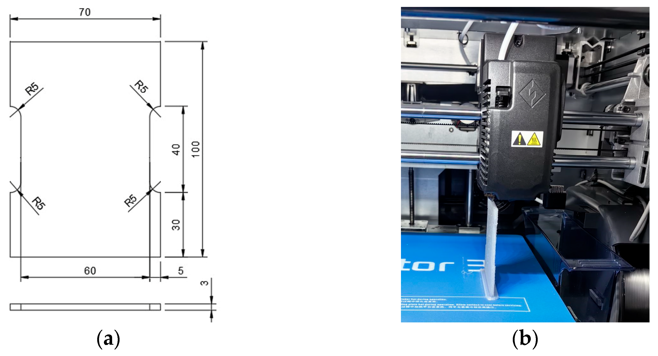
The experiment was planned using a central composite design [5]. When using such a design, the resulting mathematical regression model provides equal accuracy for all points equally distant from the center of the factor space. The design of experiment was carried out using Minitab, and the printing speed values are in the range of 40–120 mm/min and the heights of the layers are in the range of 0.1–0.4 mm. The value of α in this two-factor design is 1.41 across a total of 13 trials, with 5 trials in the center of the square. Figure 1a shows a drawing of a test specimen [6].

Figure 1.
(a) Test specimen dimensions. (b) 3D printing a specimen.
The main parameters under which the samples were printed are as follows:
- Material: PetG;
- Printing speed range: 40–120 mm/s;
- Extruder temperature range: 235 °C;
- Bed temperature: 65 °C;
- Layer height range: 0.1–0.4 mm;
- Infill: 100%;
- Flow: 103%;
- Printing time range: 25–28 min.
Thirteen samples were printed using a Flashforge Creator 3 3D printer, as shown in Figure 1b. The samples were printed vertically to investigate the connection between the layers.
Hardness tests were performed on a calibrated Shore D durometer according to ASTMD2240. The tested material was within the working range of the instrument [7]. The requirements for distances between test runs were met.
Tensile strength tests were performed on a calibrated tensile testing machine operating with a maximum possible force of 10 kN. The selected strain rate was 40 mm/min in order to obtain more precise results [8].
The optimization was performed through a regression equation, which aims to analyze the influence of the variables, both individually and interactionally. Based on the experimental results, a mathematical model was created and the statistical sample was analyzed and summarized. The model was checked for statistical significance and the coefficients of the variables in the regression equation were calculated. They were analyzed to see how well the data corresponded to the equation. The resulting mathematical model was interpreted in accordance with the physicochemical technological features of the process.
3. Results and Discussion
The experimental data from Table 1 were processed mathematically and statistically with the MINITAB software product to obtain a math model [9].

Table 1.
Obtained results.
For the mathematical description of the objective function (maximum force—F max), the following regression model was obtained [10]:
Table 2 presents the coefficient value. T-value is used to determine whether the coefficients are significant. However, the p-value is more commonly used because the threshold for rejecting the null hypothesis does not depend on the degrees of freedom. In our case, the p-value for each coefficient is lower than 0.05, so we can reject the null hypothesis. In other words, the coefficients have a lower p-value and are significant for this model [11].

Table 2.
Coefficients of the statistical equation for F max.
The calculated coefficient of determination R-sq = 99.88%, the adjusted coefficient of determination R-sq(adj) = 99.82%, and the predicted coefficient of determination has the value R-sq(pred) = 99.58% (Table 3) [12]. R-squared and adjusted R-squared are both around 99%, which means about 99% of variability in the outcome. The model fits very the model well.

Table 3.
Summary of the statistical model for Fmax.
The p-value for the F-test of the overall significance test is lower than 0.05, which gives us grounds to reject the null hypothesis and conclude that the resulting model provides a good and adequate description of the studied variable (Table 4) [13].

Table 4.
Statistical analysis of variance for F max.
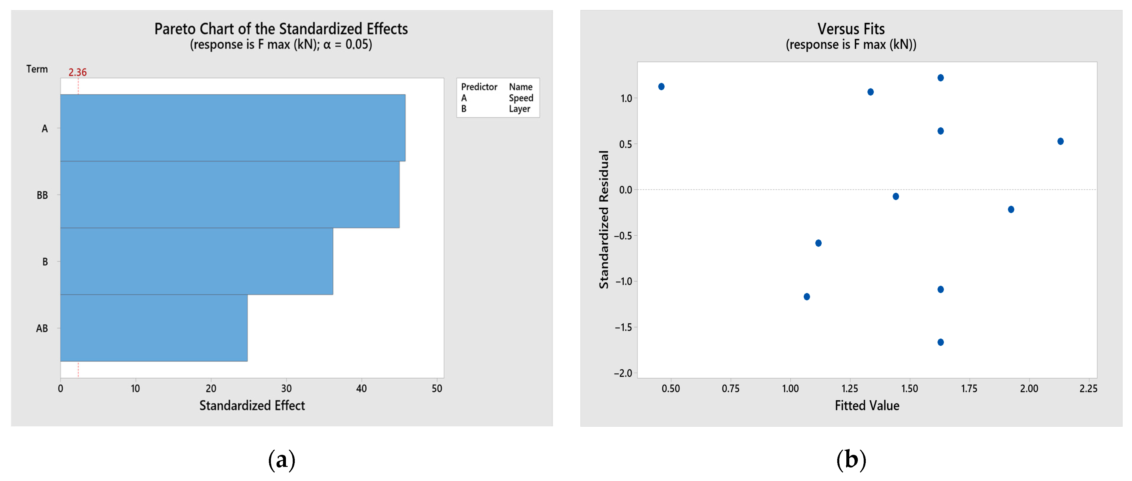
The Pareto diagram, Figure 2a, arranges the coefficients according to their effect on the desired function from largest to smallest. The diagram also draws a reference line to show where the limit of statistical significance is. It can be seen that the components pass the significance line; therefore, they are significant [14].

Figure 2.
Results: (a) Pareto diagram; (b) Standard residuals.
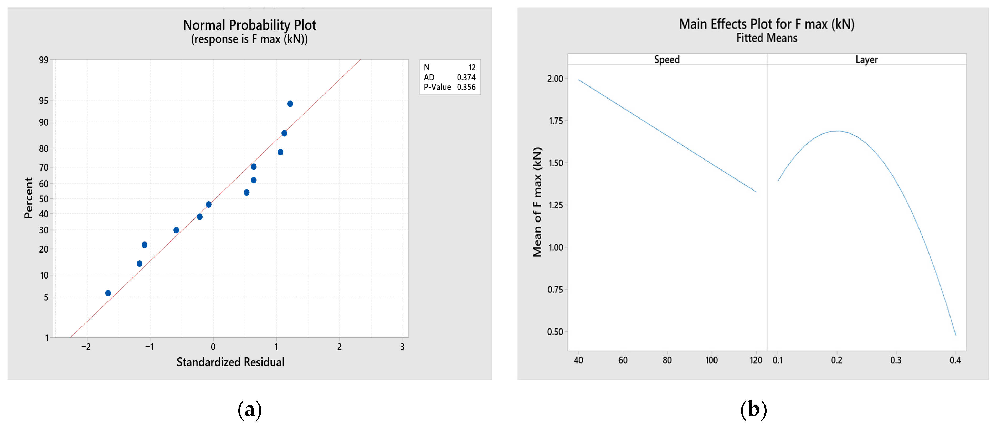
The standard residual is equal to the value of the residual divided by an estimate of its standard deviation. These residuals are useful because raw residuals may not be good indicators of a deviation in the regression model. It is clear from Figure 2b and Figure 3a that there are no gross errors in this regression model. The analysis of the residuals does not indicate a violation of the assumptions of the regression analysis. From Figure 3a, it can be seen that all residuals have an interval of ±2
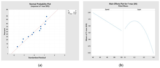
Figure 3.
Results: (a) Standardized residuals; (b) Main effects plot for F max.
The Anderson–Darling (AD) statistical test was used, which measures how well the data follow the chosen distribution [15]. The test was also used to determine the adequacy of the model. The AD test confirmed the normal distribution of the standardized residuals. The calculated AD value of 0.374 is less than the critical value of 0.683 for the sample of 12 observations and the associated p-value of 0.356 of the AD statistics is significantly above the 0.05 level. The lower value of AD compared to the critical value and the p-value ≥ α confirm a normal probability distribution of the residuals [16]. Therefore, it may be concluded that the regression model is adequate. The main effects plots, Figure 3b, show mean values for each predictor variable while keeping the other variables in the model constant. Since the lines are not horizontal, the main effects are present for speed and layers.
The results of the regression analysis confirm that all main effects are statistically significant [17]. However, because the interaction effects are statistically significant, the main effects plot can be misleading. Therefore, it cannot interpret the main effects without considering interaction effects.
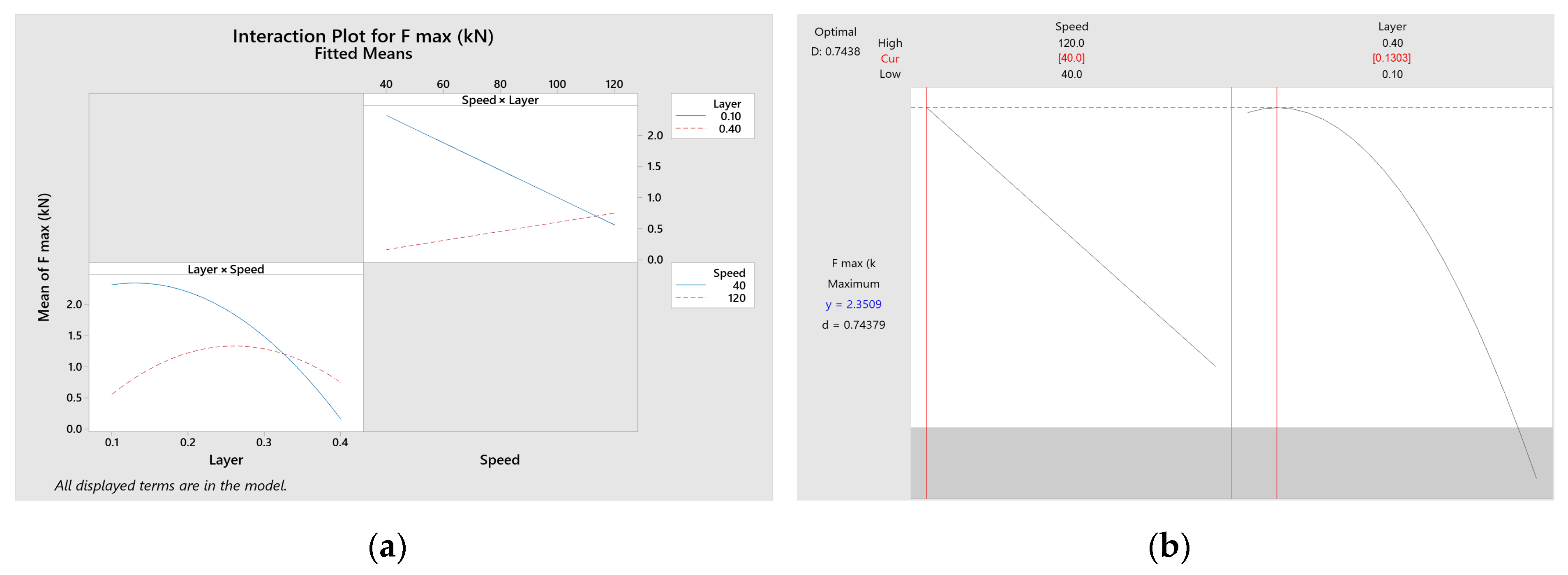
The interaction plot, Figure 4a, shows an obvious interaction effect, as the lines are not horizontal, suggesting that the maximum tensile force depends on the speed and layer height.
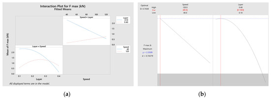
Figure 4.
Results: (a) Interaction plot for F max; (b) Optimal solution.
For technological reasons, a maximum is sought for the maximum force—F max. Based on a preliminary analysis of the experimental results, 2.4 kN was selected as a logical maximum value. A single-parameter optimization was performed and the maximum values for the objective function were found. Table 5 contains the desired response (F max), according to a defined target of 2.4 kN.

Table 5.
Parameters of the statistical model for F max.
Table 6 contains the possible solutions, according to the defined goal. Table 7 presents the best optimization fit of the variables, according to the desired response. The graphical optimization consists of plotting graphs with lines of constant values for the objective function. The results for a speed of 40 mm/s and a layer thickness of 0.13 mm were obtained, with a maximum force of 2.35 kN; they are presented in Figure 4b.

Table 6.
Solutions of the statistical model for F max.

Table 7.
Multiple response prediction for F max.
The experimental data from Table 1 for hardness (H Shore D) were also processed mathematically and statistically with the MINITAB software product, and the following regression model was obtained:
In this case, the p-value for almost every coefficient is lower than 0.05, except for Layer and Layer × Layer, so these coefficients are insignificant for this model (Table 8).

Table 8.
Coefficients of the statistical equation for hardness.
The calculated coefficient of determination R-sq = 97.06%, the adjusted coefficient of determination R-sq(adj) = 95.37%, and the predicted coefficient of determination has a value of R-sq(pred) = 90.25%, as shown in Table 9. The obtained determination fits the model very well, according to the experimental data.

Table 9.
Summary of the statistical model for hardness.
The p-value for the F-test, the overall significance test of the regression model, is lower than 0.05, which gives us grounds to reject the null hypothesis and conclude that the resulting model is adequate. There are two coefficients with slightly elevated values above 0.05, i.e., speed and Layer × Layer shown in Table 10, which do not affect the overall regression.

Table 10.
Statistical analysis of variance for hardness.
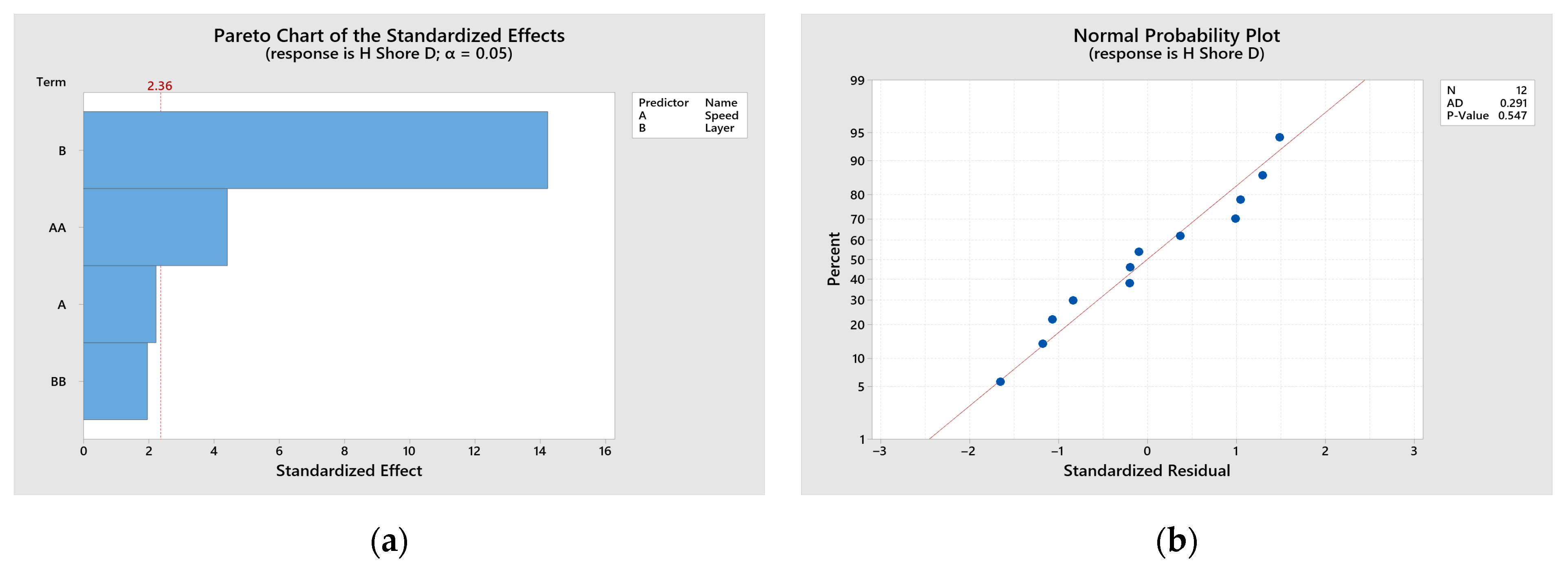
The Pareto diagram, Figure 5a, arranges the coefficients according to their effect on the objective function from the largest to the smallest [18]. The diagram also draws a reference line to show where the statistical significance limit is. It can be seen that components B and AA pass the significance line; therefore, they are significant, and the remaining A and BB are very close to it [19].

Figure 5.
Results: (a) Pareto chart; (b) Standardized residuals.
From Figure 5b, it can be seen that all standardized residuals are within an interval of ±2. The lower value of AD compared to the critical value and p-value ≥ α confirm a normal probability distribution of the residuals [20]. Therefore, it can be concluded that the regression model is adequate and the null hypothesis can be rejected.
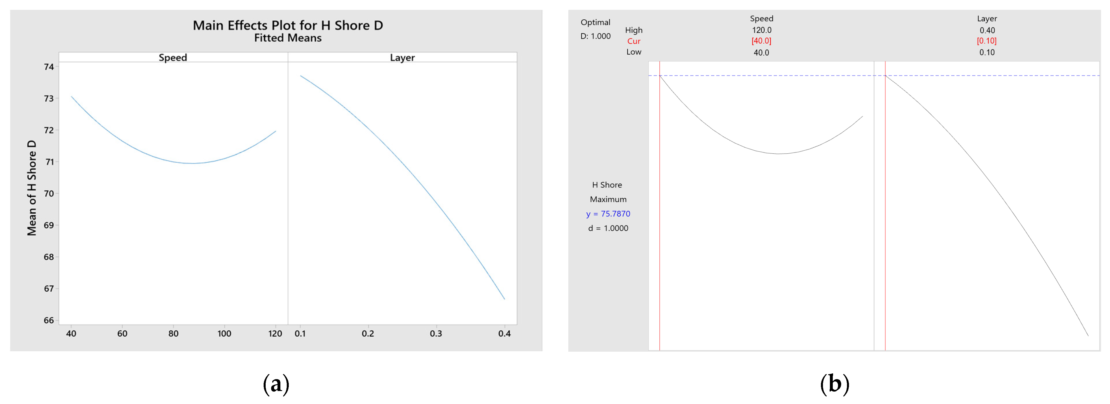
From the diagram of the main effects, Figure 6a, it can be seen that the greatest influence on the hardness is the printing layer [21].
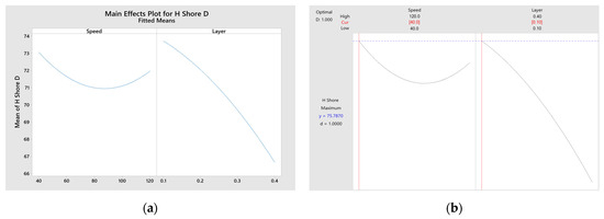
Figure 6.
Results: (a) Main effects plot for hardness Shore D; (b) Graphical presentation of the optimization.
For technological reasons, a maximum hardness—H Shore D—is sought, as shown in Table 11. A single-parameter optimization was performed, and the maximum values for the objective function were found [22]. The printing modes for four values obtained from the hardness optimization are presented in Table 12, Table 13 and Table 14.

Table 11.
Parameters of the statistical model for hardness.

Table 12.
Solutions of the statistical model for hardness.

Table 13.
Settings of variables.

Table 14.
Multiple response prediction. for hardness.
The results obtained for the graphical optimization with a speed of 40 mm/s and a layer thickness of 0.1 mm, obtaining a maximum hardness of 75.79 Shore D, are presented in Table 12.
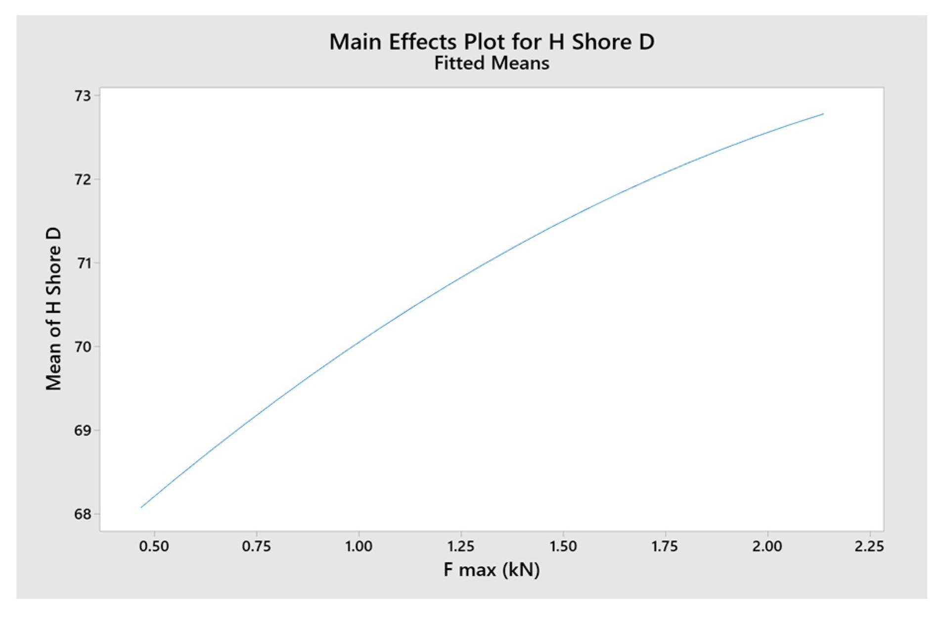
Figure 7 presents a graph of the relationship between tensile strength and hardness.
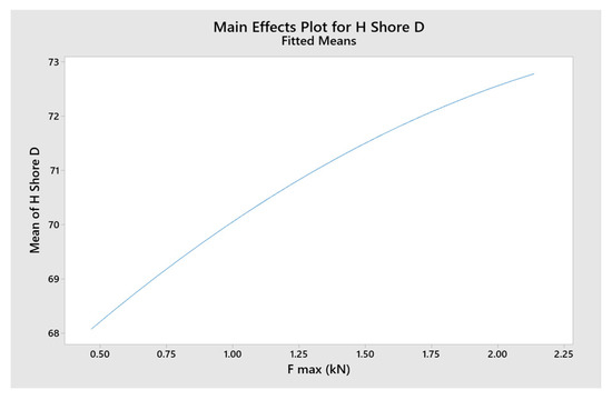
Figure 7.
Main effects plot for Hardness Shore D.
From the analysis of the experimental results, it may be concluded that the tensile strength and hardness decrease when the layer thickness increases. This is due to the higher density of defects [23]. Compared to experimental results of PLA, the decrease in strength characteristics is weaker [24]. Increasing the printing speed reduces the tensile strength because more defects are obtained due to impaired polymerization [25].
4. Conclusions
The following conclusions may be indicated:
- From the research it may be concluded that the greatest influence on tensile strength is exerted by printing speed.
- The tensile strength is highest at low speeds and small height between the layers of 3D printing.
- For the optimization with 95% probability, the printing speed is 40 mm/s, the layer height is 0.13 mm, and the tensile strength ranges from 2.30 to 2.40 kN.
- The study of the hardness shows that only the layer height factor is relevant to the hardness. The printing speed factor can be ignored as a factor.
- The hardness of the sample is highest at printed layers with small heights.
- From the optimization with 95% probability, it can be observed that at a printing speed of 40 mm/s and a 0.1 mm layer height, the hardness ranges from 74.50 to 77.07 Shore.
- It may be concluded that the 3D printing of the PetG material should be performed at the lowest possible printing speeds and the minimum possible height between the layers for maximum tensile strength and maximum hardness.
Author Contributions
Conceptualization, V.B., S.S. and K.C.; methodology, K.C.; software, S.S.; validation, V.B., S.S. and K.C.; formal analysis, V.B.; investigation, K.C.; resources, S.S.; data curation, K.C.; writing—original draft preparation, K.C.; writing—review and editing, V.B.; visualization, V.B.; supervision, V.B.; project administration, K.C.; funding acquisition, S.S. All authors have read and agreed to the published version of the manuscript.
Funding
This research was funded by the European Regional Development Fund as part of the OP “Research, Innovation and Digitalization Programme for Intelligent Transformation 2021–2027”, Project № BG16RFPR002-1.014-0005, Center of competence “Smart Mechatronics, Eco- and Energy Saving Systems and Technologies”.
Institutional Review Board Statement
Not applicable.
Informed Consent Statement
Not applicable.
Data Availability Statement
Data will be made available upon request.
Conflicts of Interest
The authors declare no conflicts of interest.
Abbreviations
The following abbreviations are used in this manuscript:
| PLA | Polylactic acid |
| ABS | Acrylonitrile butadiene styrene |
| PETG | Polyethylene terephthalate |
| PEEK | Polyether ether ketone |
| PEI | Polyethylenimine |
References
- Li, Y.; Li, X.; Shen, D. Existing 3D Printing Technologies. In Additive Manufacturing: Fundamentals and Advances; Springer: Singapore, 2024. [Google Scholar] [CrossRef]
- Xu, Y. Types and applications of 3D printing. Highlights Sci. Eng. Technol. 2024, 119, 697–702. [Google Scholar] [CrossRef]
- Nerella, M.; Kumar, R.; Naik, G.; Vinoth, R.; Ram, S.; Thakur, G.; Verma, A. Performance Evaluation of Carbon Fiber Reinforced with Polyethylene Terephthalate Glycol (PETG) in Additive Manufacturing. E3S Web Conf. 2024, 588, 01014. [Google Scholar] [CrossRef]
- Baltic, M.; Vasić, M.; Vorkapić, M.; Bajić, D.; Piteľ, J.; Svoboda, P.; Vencl, A. PETG as an Alternative Material for the Production of Drone Spare Parts. Polymers 2024, 16, 2976. [Google Scholar] [CrossRef]
- Iwundu, M. Construction of Modified Central Composite Designs for Non-standard Models. Int. J. Stat. Probab. 2024, 7, 95. [Google Scholar]
- Arhamnamazi, S.; Aymerich, F.; Buonadonna, P.; El Mehtedi, M.; Taheri, H. Application of Central Composite Design in the Drilling Process of Carbon Fiber-Reinforced Polymer Composite. Appl. Sci. 2024, 14, 7610. [Google Scholar] [CrossRef]
- Ganapathi, C.; Sunil, K.C.; Maddani, M.; Narayana, Y. A Study on Shore D Hardness of Areca Husk Fibre Reinforced Polyester Resin Composite: Impact of Fibre Maturity. Mater. Sci. Forum 2023, 1111, 83–88. [Google Scholar] [CrossRef]
- Kanlı, E.; Parmaksız, F.; Kocar, O.; Mert, F.; Anaç, N. Effect of Dimensional Differences on Tensile Strength in Tensile Test Specimens. Gazi J. Eng. Sci. 2024, 10, 619–631. [Google Scholar] [CrossRef]
- Nashrudin, I.S.; Isywatuddiyanah; Muzaffar, I. Calculation of Parameter Estimation for Two Means Using Minitab. ResearchGate Prepr. 2024, 23, 1–23. [Google Scholar] [CrossRef]
- Runkler, T. Regression. In Data Science and Machine Learning; Springer: Berlin/Heidelberg, Germany, 2024. [Google Scholar]
- Zhou, N.; Blaha, O.; Zelterman, D. Distributions and Their Approximations for p-Values. In Statistical Methods for Research; Springer: Cham, Switzerland, 2024. [Google Scholar]
- Lecca, P. Regression and Variable Selection. In Modern Statistical Modeling; Springer: Cham, Switzerland, 2024. [Google Scholar]
- Zhao, G.; Yang, J.; Zhang, L.; Yang, H. ANOVA F Test of Non-Null Hypothesis. Eur. J. Stat. 2024, 4, 4. [Google Scholar] [CrossRef]
- Funke, D.; Hespe, D.; Sanders, P.; Storandt, S.; Truschel, C. Pareto Sums of Pareto Sets: Lower Bounds and Algorithms. arXiv 2024. [Google Scholar] [CrossRef]
- Coronel-Brizio, H.; Hernandez-Montoya, A.; Rodríguez-Achach, M.; Tapia-McClung, H.; Segovia, J.T. Anderson-Darling and Watson Tests for the Geometric Distribution with Estimated Probability of Success. PLoS ONE 2024, 19, e0315855. [Google Scholar] [CrossRef]
- Qu, X. Exact Moments of Residuals of Independence. Mathematics 2024, 12, 3987. [Google Scholar] [CrossRef]
- Finkelstein, M.; Levin, B. Regression Models. In Biostatistics Handbook; Springer: New York, NY, USA, 2024. [Google Scholar]
- Ye, R.; Chen, L.; Kou, W.-B.; Zhang, J.; Ishibuchi, H. Pareto Front Shape-Agnostic Pareto Set Learning in Multi-Objective Optimization. arXiv 2024. [Google Scholar] [CrossRef]
- Fodouop Kouam, A.W. Assimilating Mediating and Moderating Variables in Academic Research: Role and Significance. Int. J. Res. Publ. 2024, 143, 273–278. [Google Scholar] [CrossRef]
- Chen, Z.; Yao, F. Matrix Completion via Residual Spectral Matching. arXiv 2024. [Google Scholar] [CrossRef]
- Andiku, C.; Lubadde, G.; Aru, J.; Ugen, A.; Ebiyau, J. Additive Main Effects and Multiplicative Interaction and Genotype Main Effect and Genotype by Environment Interaction Effects-Biplot Analysis of Sorghum Grain Yield in Uganda. J. Agric. Sci. 2024, 12, 98. [Google Scholar] [CrossRef]
- Shih, C.-J.; Ding, J.-J. A Tutorial of Optimization. ResearchGate Prepr. 2024, 222, 60–95. [Google Scholar] [CrossRef]
- Jovanić, D.; Desnica, E.; Malić, D. The Influence of the Layer Height on the Hardness of the TPU Plastic Specimen Made by 3D Printing. In Proceedings of the International Conference on Material Science, Amsterdam, The Netherlands, 26–27 September 2024; pp. 77–83. [Google Scholar] [CrossRef]
- Cahyati, S.; Furqon, Y. The Layer Height Variations Effect on Tensile Strength of 3D Printing Product PLA Material Based. J. Rekayasa Mesin 2022, 13, 647–657. [Google Scholar] [CrossRef]
- Loskot, J.; Jezbera, D.; Loskot, R.; Bušovský, D.; Barylski, A.; Glowka, K.; Duda, P.; Aniołek, K.; Voglová, K.; Zubko, M. Influence of Print Speed on the Microstructure, Morphology, and Mechanical Properties of 3D-Printed PETG Products. Polym. Test. 2023, 123, 108105. [Google Scholar] [CrossRef]
Disclaimer/Publisher’s Note: The statements, opinions and data contained in all publications are solely those of the individual author(s) and contributor(s) and not of MDPI and/or the editor(s). MDPI and/or the editor(s) disclaim responsibility for any injury to people or property resulting from any ideas, methods, instructions or products referred to in the content. |
© 2025 by the authors. Licensee MDPI, Basel, Switzerland. This article is an open access article distributed under the terms and conditions of the Creative Commons Attribution (CC BY) license (https://creativecommons.org/licenses/by/4.0/).

