Approximation of Dynamic Systems Using Deep Neural Networks and Laguerre Functions ^†

Abstract

This article presents a hybrid approach that combines Laguerre orthonormal functions with deep neural networks (DNN) for effective approximation of impulse responses of dynamic systems. Attention is given to key limitations in approximation with Laguerre functions, such as the selection of the optimal scaling factor, the number of functions used, and computational complexity. By training compact DNNs that directly predict the decomposition coefficients, increased functionality is achieved, as well as greater flexibility and efficiency in the context of implementing MPC. The proposed architecture provides good scalability, robustness, and computational efficiency, making it applicable in tasks related to system approximation and identification under uncertainty and noise conditions.

1. Introduction

In the last decade, elements of artificial intelligence have been used almost everywhere to solve various tasks. Deep neural networks (DNNs) have emerged as a very powerful tool. They are used in a variety of applications such as image processing and recognition [1,2], process prediction [3], solving mathematical problems [4], optimal control [5], intelligent control of robotic systems [6], energy system management [7], workers’ safety [8], and many others.

Their technical success is mainly due to their computational efficiency, but they also possess other properties such as automatic feature extraction, good generalization ability, flexible architecture, easy combination with other approaches, and more. Function approximation is one of the tasks in which DNNs show remarkable results. The approximation of functions or systems through their characteristics is a widely spread problem in various engineering fields [9,10,11], and new and reliable approaches are constantly being sought to achieve better results. Deep neural networks can approximate various functions in high dimensionality with arbitrary precision due to their expressive capabilities.

In approximation tasks, DNNs have a number of advantages and outperform classical numerical methods and even conventional (shallow) neural networks [12,13,14]. They overcome the so-called curse of dimensionality (COD). This term refers to the exponential degradation of results as dimensionality increases. Several studies provide explanations for the approximation properties of DNNs, such as the role of compositionality [15], approximation in appropriate functional spaces [16], the manifold hypothesis [17,18], and more.

Other advantages include their ability to provide both local and sparse approximation [12], for which the neural network must have at least two hidden layers. The use of the ReLU activation function and, consequently, deep ReLU networks, demonstrates better generalization capabilities [19]. Another key issue is saturation. Early research in this area reached the conclusion that this problem exists in all types of artificial neural networks [20], while [21] presents neural networks with controllable weight norms that can approximate one-dimensional functions without saturation.

A fundamental conclusion when determining the choice of DNN for solving a given problem, particularly function approximation, is the architecture of the network itself. In approximation theory, the topic of constructing DNNs is widely discussed and forms the basis for achieving good results. Another commonly used approach in modern AI implementation is breaking down a complex task into several simpler ones, leading to efficiency both in training and subsequent computations, which allows for applications in real-time autonomous systems and even real-time control.

In the literature, there are many known methods for approximation, and the set of methods is extremely large, making it impossible to cover all of them. However, the most frequently studied groups are: analytical methods, numerical methods for approximation, series expansion methods, and approximation based on intelligent methods.

The task of approximation applied to systems is highly significant, as it offers the replacement of the original system model with a simpler one while maintaining a sufficiently accurate representation in accordance with the defined objectives. Among all the approaches used for system approximation, an important class of functions for approximation are orthonormal functions. Any linear system with constant parameters can be approximated by an infinite series of such functions, which may include one or more free parameters. A key representativ e of this type of special functions that meet the necessary requirements are the Laguerre functions.

Laguerre orthonormal functions are traditionally used in the synthesis of model-predictive controllers and other similar applications [22,23,24,25]. Decomposition of continuous and discrete systems using a set of Laguerre functions is also applied in computational tasks in mathematical physics [26] for approximation and asymptotic analysis [27], reduction in system order with time delays [28], system identification [29], extension of spectral methods with applications in nuclear magnetic resonance [30], and many others.

Relatively less attention has been given to the use or rather the combination of orthonormal functions and artificial neural networks (ANNs). In terms of combining Laguerre functions and ANNs, two main directions can be distinguished:

-

Integration of Laguerre orthonormal functions into the structure of ANNs [31,32,33,34]

-

Integration of ANNs into the Laguerre network [35,36,37]

In this article, the issue of approximating impulse (transient) characteristics of systems is addressed by using orthonormal Laguerre functions and deep neural networks (DNNs), with the aim of optimizing the process of generating the set of Laguerre functions for noisy systems with parametric uncertainties.

2. Material and Methods

2.1. Problem Statement

Based on the presented literature review, it is clear that orthonormal Laguerre functions are primarily applied in the synthesis of model predictive controllers (MPC). When designing an MPC using Laguerre functions, which is based on modeling the control signal, i.e., solving a time-function approximation problem, new challenges arise from production constraints. These challenges pertain to both the approximation process and the synthesis of the controller itself, and include the following main aspects:

-

Selection of the time scaling factor—although the influence of this parameter on orthonormal functions has been well studied, there is no universal method for determining it, especially in the context of approximation tasks.

-

Determining the number of orthonormal functions—although a definition for the completeness of the set of orthonormal functions exists [35], it assumes a finite number of functions for approximation. However, excessively increasing this number leads to significant computational complexity. It is necessary to find the optimal number of functions that is sufficient for an accurate representation of a system of a given order.

-

Calculation of the decomposition coefficients—this process is computationally intensive, especially when implementing MPC with a long prediction horizon, using adaptive basis functions, or dealing with objects exhibiting parametric uncertainty and noise. In such cases, continuous recalculation of the coefficients can complicate the application of the method. The problem is further exacerbated by the fact that Laguerre orthonormal functions cannot directly approximate the transient characteristics of open systems.

The solution to these problems can be achieved by using DNNs, thereby avoiding additional complications such as: computational inefficiency, both during training and operation; saturation and overfitting; and forgetting.

2.2. Laguerre Orthonormal Functions

The orthonormal decomposition using Laguerre functions is described in detail in [38]. Avoiding strict mathematical descriptions in Hilbert space, a function must satisfy the conditions for orthonormality, i.e., each function in the set must be orthogonal to every other function and have a norm equal to 1:

$${\int }_0^{\infty }{l}_i\left(t\right)l_j\left(t\right)dt=\left\{\begin{array}{c}1, if i=j\\ 0, if i\ne j\end{array}\right.$$

(1)

where $l_i\left(t\right)$ is a set of real functions, with i, j = 1,2,3 … in [0,∞).

A set of orthonormal functions $l_i\left(t\right)$ is complete if the condition:

$${\int }_0^{\mathrm{\infty }}f\left(t\right)l_i\left(t\right)dt=0$$

(2)

can be satisfied for all values of $i$ only if the square of the function $f\left(t\right)$ satisfies:

$${\int }_0^{\infty }f{\left(t\right)}^{2}dt=0$$

(3)

If a set of functions satisfies conditions (2) and (3), they can be used to approximate any function, similar to a Fourier series expansion [39].

An arbitrary function f(t) can be approximated arbitrarily closely with an increasing number of terms N using:

$$f\left(t\right)=\sum _{i=1}^N{c}_i{l}_i\left(t\right).$$

(4)

The general form of the decomposition coefficients $c_i=\mathrm{1,2},3,\dots$ is determined by:

$$c_i={\int }_0^{\infty }{l}_i\left(t\right)f\left(t\right)dt$$

(5)

The Laguerre functions are a set of orthonormal functions that satisfy conditions (2) and (3) and are defined for each p > 0 as:

$$\begin{array}{c}{l}_1\left(t\right)=\sqrt{2p}\times e^{-pt}\\ l_2\left(t\right)=\sqrt{2p}(-2pt+1)\times e^{-pt}\\ ..........\\ l_i\left(t\right)=\sqrt{2p}{\displaystyle \frac{e^{pt}}{(i-1)!}}{\displaystyle \frac{d^{i-1}}{d{t}^{i-1}}}\left[t^{i-1}{e}^{-2pt}\right]\end{array}$$

(6)

where p is called the scaling factor.

The scaling factor determines the exponential decay of the Laguerre functions and serves as a user-defined parameter, which is set depending on the application (approximation, MPC, identification, or others).

The formation of the network of Laguerre functions is performed by applying the Laplace transform to the set of functions:

$$\begin{array}{c}{L}_1\left(s\right)={\int }_0^{\infty }{l}_1\left(t\right)e^{-st}dt={\displaystyle \frac{\sqrt{2p}}{\left(s+p\right)}}\\ L_2\left(s\right)={\int }_0^{\infty }{l}_2\left(t\right)e^{-st}dt={\displaystyle \frac{\sqrt{2p}\left(s-p\right)}{{\left(s+p\right)}^2}}\\ .........\\ L_i\left(s\right)={\int }_0^{\infty }{l}_i\left(t\right)e^{-st}dt={\displaystyle \frac{\sqrt{2p}{\left(s-p\right)}^{i-1}}{{\left(s+p\right)}^i}}\end{array}$$

(7)

where $L_i\left(s\right)$ are also called Laguerre filters, and by sequentially connecting them, they form a Laguerre network.

The generation of Laguerre functions can be performed using (6) or (7), but it is more practical to do so by representing them in state space. This form is more compact, especially considering its application in MPC synthesis. The orthonormal Laguerre functions are represented in state space form in detail in [38], where the state vector is first chosen as $L\left(t\right)={\left[\begin{array}{cccc}{l}_1\left(t\right)& l_2\left(t\right)& ...& l_N\left(t\right)\end{array}\right]}^T$. The initial states of the variables from this vector are $L\left(0\right)=\sqrt{\left(2p\right)}{\left[\begin{array}{cccc}1& 1& ...& 1\end{array}\right]}^T$, and they are then obtained after solving the equation:

$$\left[\begin{array}{c}{i}_1\left(t\right)\\ i_2\left(t\right)\\ ...\\ i_N\left(t\right)\end{array}\right]=\left[\begin{array}{cccc}-p& 0& \dots & 0\\ -2p& -p& \dots & 0\\ ⋮& \ddots & \ddots & ⋮\\ -2p& \dots & -2p& -p\end{array}\right].\left[\begin{array}{c}{l}_1\left(t\right)\\ l_2\left(t\right)\\ ...\\ l_N\left(t\right)\end{array}\right]$$

(8)

In Figure 1a,b, the graphs of the Laguerre functions for N = 6 are presented, with p = 1 and p = 4, i.e., the first six functions, implemented in the MATLAB environment.

As the scaling factor increases, the Laguerre orthonormal functions must decay exponentially at a faster rate, as seen in the presented graphs in Figure 1.

2.3. Approximation of Systems Using Laguerre Functions

Laguerre functions are widely used for the approximation and identification of systems. In the literature, system approximation refers to the approximation of the transient or impulse response of a given system. When using orthonormal Laguerre functions, approximating the transient response is not directly possible, as Laguerre functions are used only for exponentially decaying functions, such as the impulse response.

In the problem of approximating the characteristics of a system, it is assumed that we do not always have an ideal mathematical model of the system. Usually, identification is based on the transient response, which is obtained experimentally, and its parameters are determined using some of the known methods [40]. From the transient response, the impulse response can be obtained, and vice versa, using the following relationships:

$$h\left(t\right)={\displaystyle \frac{dy\left(t\right)}{dt}}, for y\left(t\right)\to h\left(t\right)$$

(9)

$$y\left(t\right)={\int }_0^{t}h\left(\tau \right)d\tau , for h\left(t\right) \to y\left(t\right)$$

(10)

where y(t) is the transient response, h(t) is the impulse response.

Since using (9) and (10), it is always possible to transition from one characteristic to the other, the idea behind approximating a system with orthonormal functions is to work with the impulse response. The impulse response is represented as an orthonormal decomposition using Laguerre functions in the following way:

$$h\left(t\right)=c_1{l}_1\left(t\right)+c_2{l}_2\left(t\right)+\cdots +c_i{l}_i\left(t\right)$$

(11)

The condition for Equation (11) to be valid is that the impulse function must satisfy the condition for L2 stability, i.e., all poles of the system must be located in the left half of the complex plane and the condition for $h\left(t\right)$ must be satisfied:

$${\int }_0^{\infty }{h}^2\left(t\right)dt<\infty$$

(12)

For this type of systems, for $\epsilon >0$, there exists a number N indicating the number of orthonormal functions used, such that:

$${{\int }_0^{\infty }\left(h\left(t\right)-\sum _{i=1}^N{c}_i{l}_i\left(t\right)\right)}^{2}dt< \epsilon$$

(13)

From condition (13), it can be seen that the accuracy of the approximation will increase with the increase in N for every value of the scaling factor p > 0. If the function h(t) is known, the optimal coefficients ci can be found by minimizing the objective function from (13). Taking into account the orthonormal property of the Laguerre functions, the coefficients are found using Formula (5), where the function f(t) is the impulse response h(t)).

$$\begin{array}{c}{c}_1={\int }_0^{\infty }{l}_1\left(t\right)h\left(t\right)dt\\ c_2={\int }_0^{\infty }{l}_2\left(t\right)h\left(t\right)dt\\ \dots \dots \dots \\ c_N={\int }_0^{\infty }{l}_N\left(t\right)h\left(t\right)dt\end{array}$$

(14)

This is where the problem arises if the impulse response is not explicitly given. Typically, other methods and criteria are used to optimally determine the decomposition coefficients.

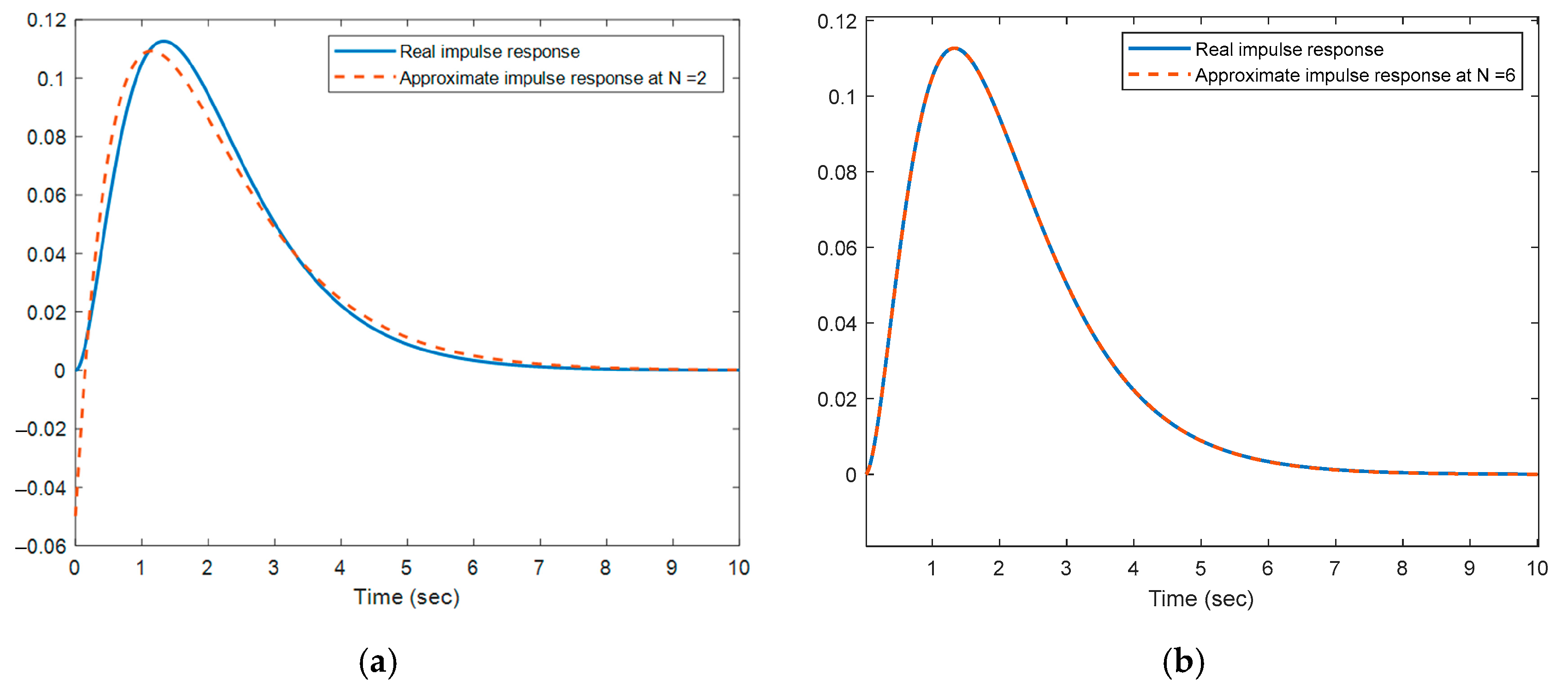
Figure 2 shows the approximated and actual impulse responses obtained from the system’s transfer function $G(s)={\displaystyle \frac{1}{(s+1.1)(s+2.4)(1+1.3)}}$, for N = 2 and N = 6.

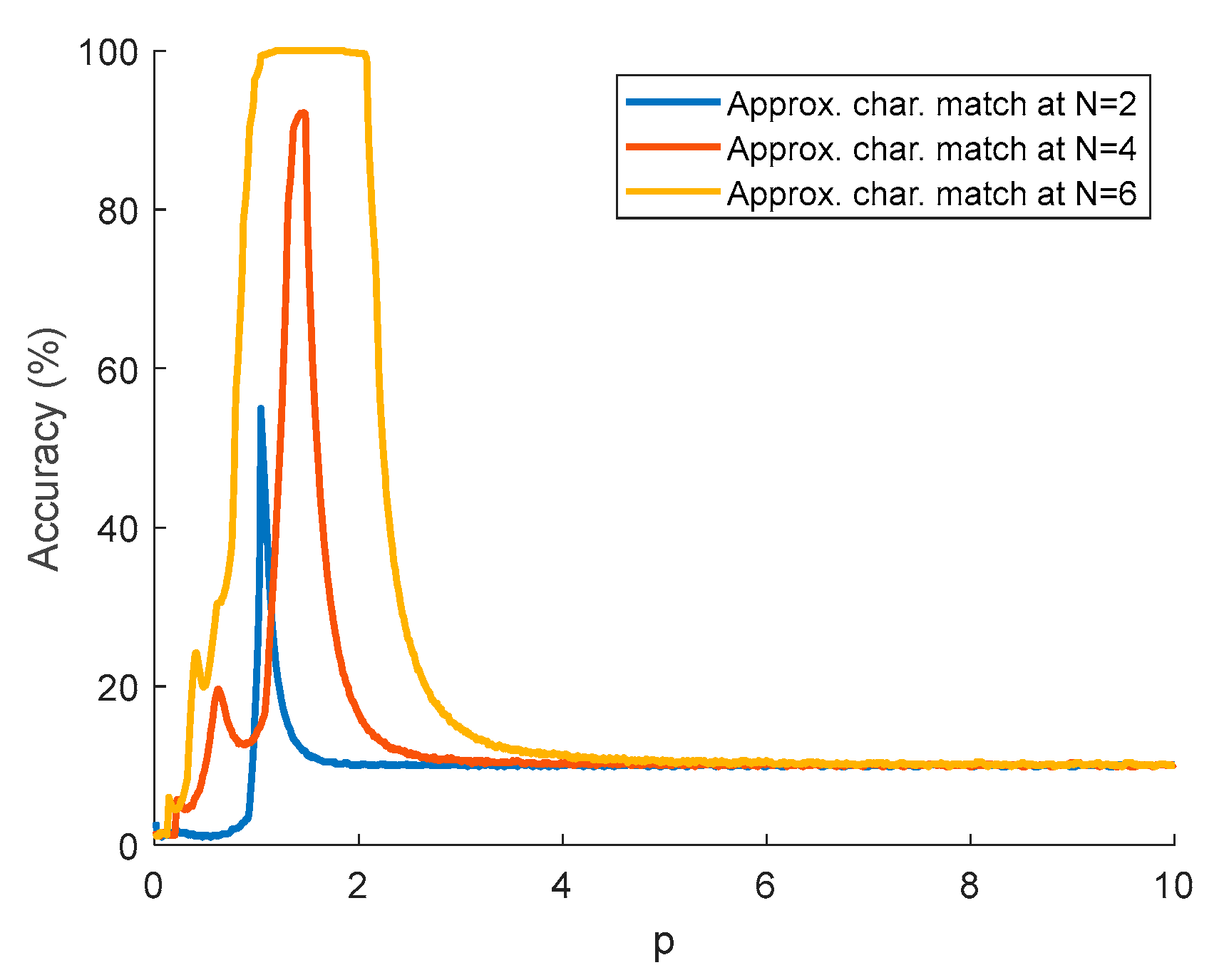
Figure 3 shows the graphs of the matching between the real and approximated impulse responses as the scaling factor p is varied from 0 to 10 with a step of 0.01, at a tolerance level of 0.001.

The graph shows that ensuring faster decay of the set of functions does not always lead to better results in terms of the approximation error. When a small number of orthonormal functions are used, the choice of scaling factor plays a key role in achieving a good result.

2.4. Approximating Systems Using Laguerre Functions and DNN

It is well-known that DNNs provide very good results in function approximation. Unfortunately, however, their computational activity makes them unsuitable for solving approximation tasks in the control loop, such as in the implementation of MPC for processes with fast dynamics.

For this reason, in the current implementation, the use of DNN is based on approximating (memorizing) not the system’s characteristic, but the orthonormal Laguerre functions and subsequently generating the decomposition coefficients. This is a much easier task, involving generating 2–6 numbers rather than generating an entire vector of values describing the whole impulse response. Using DNN in this way is rational when working with the network itself. The advantage of DNNs lies in their extensive architecture and the fundamental requirement for a large set of training data. These features somewhat prevent the phenomenon of “forgetting.” However, this does not mean that this disadvantage is typical only for conventional neural networks; DNNs also exhibit this, but to a much lesser extent. As a certain level of prevention, the Experience Replay method [38] is applied, where small portions of old data are used together with new data during training, which keeps the previous tasks “active” in the network.

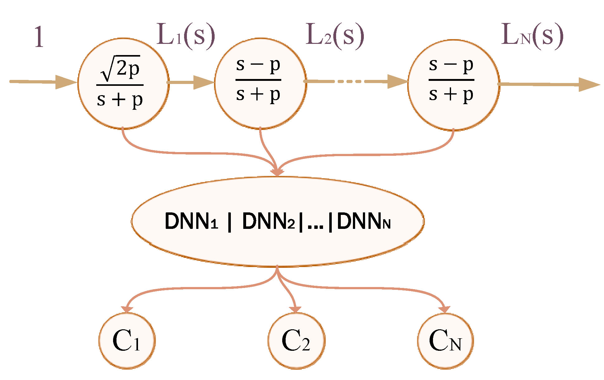
The network used in this way becomes overly large, considering the added multi-layer structure, the greater number of neurons, and the number of input neurons, which is also not small given the number of values that can be obtained for a given characteristic. The data format for DNN requires packaging, etc. For this reason, the solution to this problem is based on using several small DNNs to generate each decomposition coefficient individually. This leads to easier formation of training data, faster learning, and quicker operation of the entire software system, as the coefficients are calculated sequentially anyway. During training, the neural network does not need to cover the dependency between the different Laguerre functions (for example, between the first and second, etc.), and the desired data set consists of the values of the decomposition coefficients, with input data from the same Laguerre function, obtained for different values of the system parameters, while the set parameter uncertainties are significantly higher than expected. Figure 4 shows a block diagram of a Laguerre network and the connection of neural networks within it.

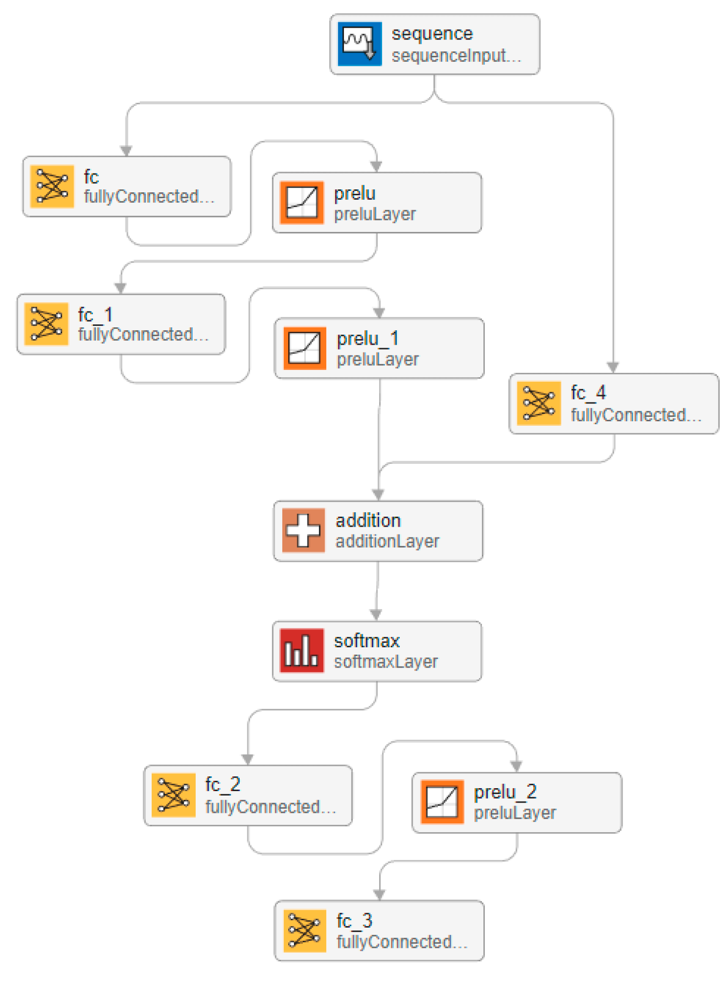
The task that DNN has to perform, as defined, cannot be attributed either to approximation tasks or to classification tasks, but rather to a feature discovery task. However, the presentation of values from numerical series as a data set is more typical of artificial networks with Sequence input layer, as used in the current case. Figure 5 shows the architecture of the used neural networks in the Matlab Deep Network Designer environment.

The designed DNN has a structure that can be conditionally divided into 4 parts: Input layer, Primary processing, Summarization block and output block.

The input layer uses sequenceInputLayer, which is a suitable layer for time-dependent data sequences.

In the part called primary processing, two parallel branches are implemented. The first consists of a serial connection of fullyConnectedLayer in combination with Parametric ReLU, with 128 neurons in the first and 64 in the second, respectively. The use of PReLU (Parametric ReLU) allows the network to flexibly adapt the slope at negative values, which improves the overall expressiveness of the network. It also makes the network more suitable for approximating complex and nonlinear functions, such as orthonormal functions, especially of higher order. In the second branch, only one fully ConnectedLayer with 64 neurons is used.

The two branches merge, resulting in a residual structure (residual path), which allows the depth of the network to grow without losing gradient, improves trainability and stability during training and keeps information from earlier layers active. This is implemented by using an additionLayer.

In the generalization part after the merger, a softmaxLayer is used, the purpose of which is to achieve controlled weighting of values and a kind of transformation. Together with the additionLayer, it allows combining different levels of abstraction and achieves sufficient depth and parameterization, which allows for universal approximation. The network becomes neither too shallow (which would limit its capabilities) nor too deep (which would make training difficult).

The output block consists of two fullyConnectedLayer with a Parametric ReLU between them, with 16 neurons for the first and one neuron for the second layer, respectively. This is a classic final stage with nonlinearity, suitable for deriving the approximated value.

3. Simulation Results and Analyses

The proposed architecture of the software system shown in Figure 4 has been implemented and tested in a Matlab environment. The procedure is implemented in several steps:

• Generation of Laguerre functions—usually up to 10 are sufficient depending on the order of the approximated system.
• The impulse characteristics of the selected system are calculated—their number depends on the number of parameters, the degree of the assumed parametric uncertainty and the step of change for the parameters. A set of characteristics is generated when fully combining the possible combinations of uncertainties. Subsequently, the procedure is repeated with noise included at different levels.
• The data for training the DNN is formed—Simpson’s algorithm is used to calculate a definite integral, which gives better accuracy compared to other simplified methods. N input data arrays are formed with the size of the number of values of the function and the number of training samples obtained. For the desired result, a one-dimensional array with the decomposition coefficients is again formed.
• Training of neural networks—Neural networks are trained using the ADAM optimizer. The maximum number of epochs is 4500, InitialLearn-Rate = 1 × 10⁻⁵, and GradientThreshold = 0.001. The values of these parameters provide a short training time, while stabilizing it, which is very important for approximating complex functions and prevents an explosive gradient, which is especially useful in DNNs. Usually, in the training process, a percentage ratio is chosen of what part of the data is used for training (those that are fed to the DNN during training) and validation (used to measure the state to stop training). The percentage ratio used is 85% for training and 15% for validation.

The implementation of approximation with orthonormal functions and DNN for generating decomposition coefficients is tested with the impulse characteristics of an example system described by its transfer function. For the system it is of second order with the transfer function:

$$G(s)={\displaystyle \frac{1}{(s+1.1)(s+2.4)}}$$

(15)

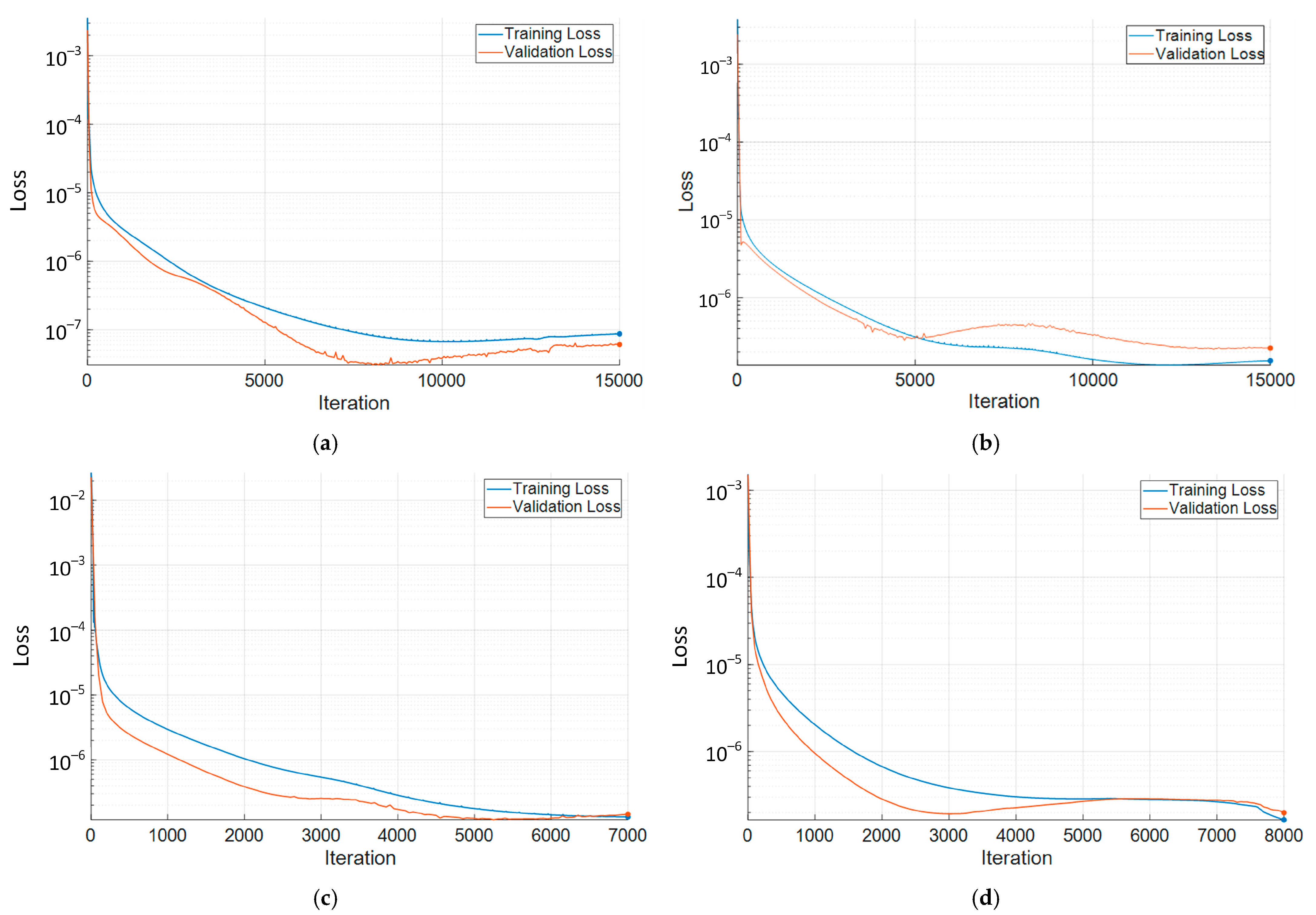
The impulse response is approximated by a 4th order Laguerre network (N = 4 and p = 1.6), and four neural networks for the four coefficients, respectively. A 50% parametric uncertainty of the two parameters is assumed. The total training sample size is 34 different functions with a calculation accuracy of 0.001. In Figure 6a–d the graphs of the training errors with the training data of the four neural networks together with the validation are shown. The number of neurons in the layers does not change. The training process is relatively short, the lowest error is achieved on average for 1000 ÷ 2000 epochs, depending on which order the training is performed for.

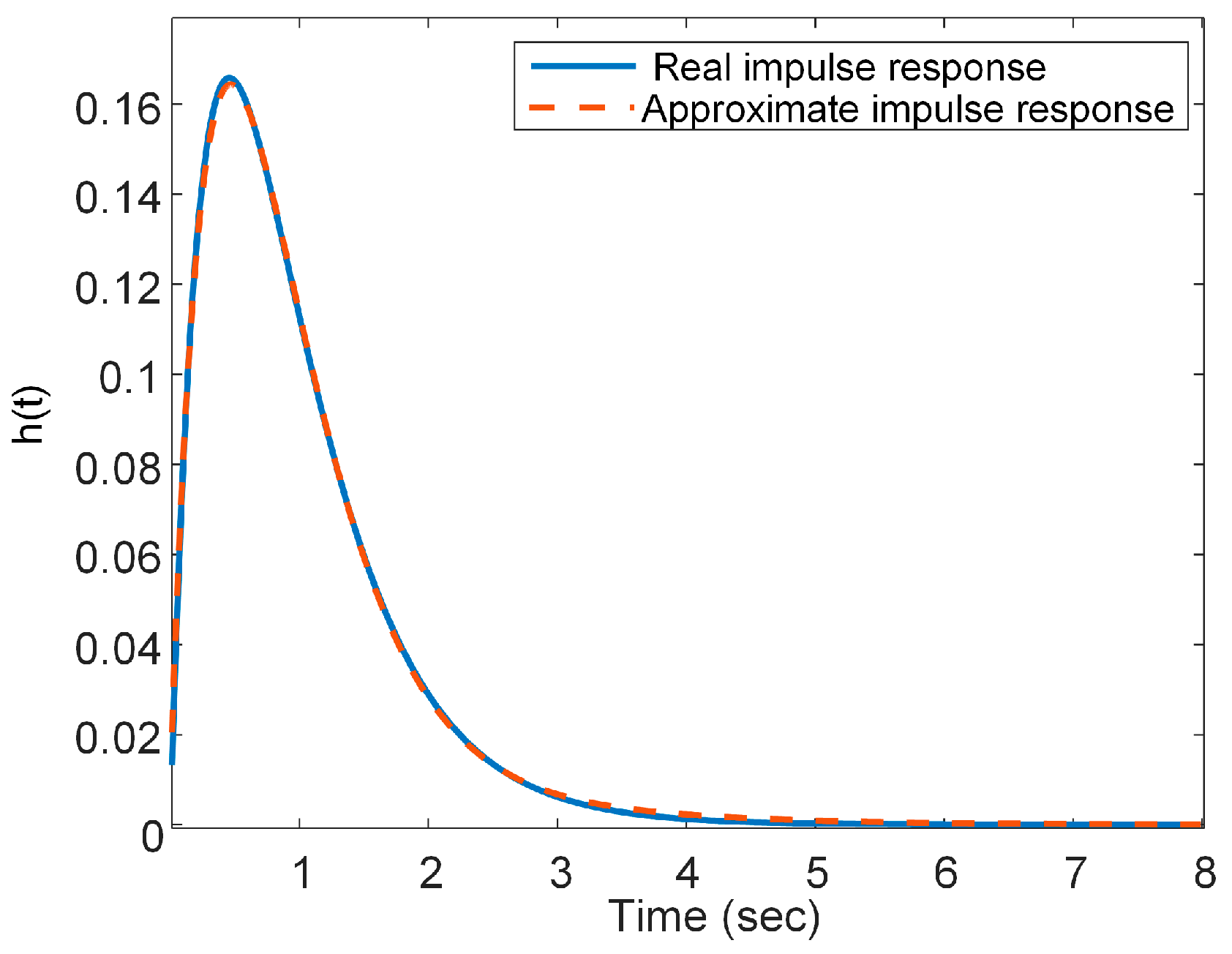
Figure 7 shows a graph of the approximation of the system with the coefficients generated by the neural networks.

Figure 8 shows the graphs of the error in training the same neural network by size and structure with data obtained with random noise in the family of impulse characteristics of the system represented by (15). Thus, the training data include both parametric uncertainties (up to 50%) and noise in the range from 0 to 5%.

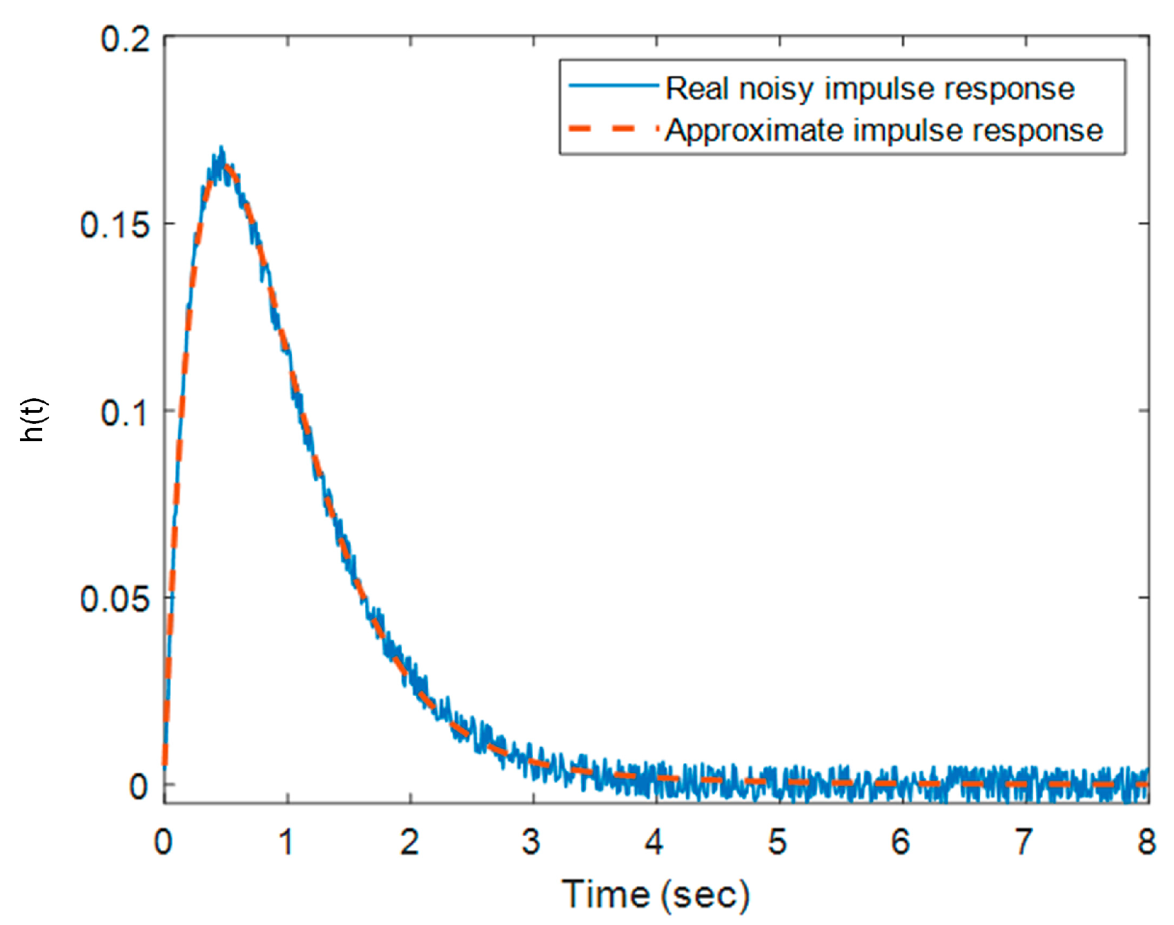
Figure 9 shows the result of approximating the noisy characteristic with the values of the coefficients obtained from the neural network.

The obtained graphical results and the tests performed show that the use of DNN gives very good results in generating decomposition coefficients in the approximation with orthonormal Laguerre functions. Successful training of the neural networks is shown, with good convergence of the errors achieved. Testing and validation show compliance and lack of significant oversaturation. The achieved mean square error (MSE), which is of the order of 1 × 10⁻⁶, provides information that the DNN successfully learns the patterns in the data during the training epochs. Validation shows the error on a separate set of data that is not directly involved in training. It can be used as a criterion for stopping training and shows that DNN does not oversaturate, i.e., the neural network has the ability to generate appropriate decomposition coefficients when working with new data of other orthonormal functions.

4. Conclusions

This paper presents a variant for approximating the impulse response of dynamic systems using orthonormal Laguerre functions combined with deep neural networks (DNNs) to generate the decomposition coefficients. The main challenges in approximation with Laguerre functions—such as the choice of a scaling factor, determining the number of orthonormal functions and the computational intensity of finding the coefficients—are overcome by an approach based on machine learning. Instead of directly approximating the entire system characteristic, DNNs are trained to generate a small number of coefficients for the Laguerre decomposition, which significantly reduces the computational complexity and makes the approach applicable to the synthesis of MPCs.

The proposed neural architecture, implemented in MATLAB, shows a stable learning process, good generalization ability and low sensitivity to noise and parametric uncertainties. The use of several small-sized DNNs for each individual coefficient leads to faster learning, easy generation of training data and a reduced risk of oversaturation. The achieved mean square error (MSE) of the order of 1.10–6 indicates high accuracy in learning the relationship between input functions and decomposition coefficients. Validation with new, unknown data confirms that the trained networks generalize successfully and can be used to approximate new systems different from the training examples. The used methodology successfully combines the analytical power of Laguerre functions with the flexibility of deep learning, providing a precise and efficient solution for function approximation in conditions of noise and uncertainty.

References

1. Wang, Y.; Tang, L.; Wen, J.; Zhan, Q. Recognition of concrete microcrack images under fluorescent excitation based on attention mechanism deep recurrent neural networks. Case Stud. Constr. Mater. 2024, 20, e03160. [Google Scholar] [CrossRef]
2. Yu, Y.; Zhang, Y.; Cheng, Z.; Song, Z.; Tang, C. MCA: Multidimensional collaborative attention in deep convolutional neural networks for image recognition. Eng. Appl. Artif. Intell. 2023, 126, 107079. [Google Scholar] [CrossRef]
3. Zhao, M.; Li, S.; Chen, H.; Ling, M.; Chang, H. Distributed solar photovoltaic power prediction algorithm based on deep neural network. J. Eng. Res. 2024; in press. [Google Scholar] [CrossRef]
4. Xu, Z.-Q.J.; Zhang, L.; Cai, W. On understanding and overcoming spectral biases of deep neural network learning methods for solving PDEs. arXiv 2025, arXiv:2501.09987. [Google Scholar] [CrossRef]
5. Chen, J.; Mei, J.; Hu, J.; Yang, Z. Deep neural networks-prescribed performance optimal control for stochastic nonlinear strict-feedback systems. Neurocomputing 2024, 610, 128633. [Google Scholar] [CrossRef]
6. Aydogmus, O.; Gullu, B. Implementation of singularity-free inverse kinematics for humanoid robotic arm using Bayesian optimized deep neural network. Measurement 2024, 229, 114471. [Google Scholar] [CrossRef]
7. Wang, M.; He, J.; Zheng, L.; Alkhalifah, T.; Marzouki, R. Optimizing Energy Capacity, and Vibration Control Performance of Multi-Layer Smart Silicon Solar Cells Using Mathematical Simulation and Deep Neural Networks. Aerosp. Sci. Technol. 2025, 159, 109983. [Google Scholar] [CrossRef]
8. Balaji, T.S.; Srinivasan, S. Detection of safety wearable’s of the industry workers using deep neural network. Mater. Today Proc. 2023, 80, 3064–3068. [Google Scholar] [CrossRef]
9. Cadoret, A.; Goy, E.D.; Leroy, J.M.; Pfister, J.L.; Mevel, L. Linear time periodic system approximation based on Floquet and Fourier transformations for operational modal analysis and damage detection of wind turbine. Mech. Syst. Signal Process. 2024, 212, 111157. [Google Scholar] [CrossRef]
10. Discacciati, N.; Hesthaven, J.S. Model reduction of coupled systems based on non-intrusive approximations of the boundary response maps. Comput. Methods Appl. Mech. Eng. 2024, 420, 116770. [Google Scholar] [CrossRef]
11. Moya, A.A. Low-frequency approximations to the finite-length Warburg diffusion impedance: The reflexive case. J. Energy Storage 2024, 97, 112911. [Google Scholar] [CrossRef]
12. Liu, X. Approximating smooth and sparse functions by deep neural networks: Optimal approximation rates and saturation. J. Complex. 2023, 79, 101783. [Google Scholar] [CrossRef]
13. Noguer, I.A. Dimensional Constraints and Fundamental Limits of Neural Network Explainability: A Mathematical Framework and Analysis. 2025. Available online: https://ssrn.com/abstract=5095275 (accessed on 13 January 2025).
14. Lin, S.-B. Limitations of shallow nets approximation. Neural Netw. 2017, 94, 96–102. [Google Scholar] [CrossRef]
15. Berner, J.; Grohs, P.; Kutyniok, G.; Petersen, P. The modern mathematics of deep learning. arXiv 2021, arXiv:2105.04026 78. [Google Scholar]
16. Siegel, J.W.; Xu, J. Characterization of the variation spaces corresponding to shallow neural networks. Constr. Approx. 2023, 57, 1109–1132. [Google Scholar] [CrossRef]
17. Fefferman, C.; Sanjoy, M.; Hariharan, N. Testing the manifold hypothesis. J. Am. Math. Soc. 2016, 29, 983–1049. [Google Scholar] [CrossRef]
18. Shaham, U.; Cloninger, A.; Coifman, R.R. Provable approximation properties for deep neural networks. Appl. Comput. Harmon. Anal. 2018, 44, 537–557. [Google Scholar] [CrossRef]
19. Han, Z.; Yu, S.; Lin, S.B.; Zhou, D.X. Depth Selection for Deep ReLU Nets in Feature Extraction and Generalization. IEEE Trans. Pattern Anal. Mach. Intell. 2022, 44, 1853–1868. [Google Scholar] [CrossRef]
20. Lin, S.-B. Generalization and expressivity for deep nets. IEEE Trans. Neural Netw. Learn. Syst. 2018, 30, 1392–1406. [Google Scholar] [CrossRef]
21. Chui, C.K.; Lin, S.-B.; Zhou, D.-X. Deep neural networks for rotation-invariance approximation and learning. Anal. Appl. 2019, 17, 737–772. [Google Scholar] [CrossRef]
22. Yan, Y.; Tang, M.; Wang, W.; Zhang, Y.; An, B. Trajectory tracking control of wearable upper limb rehabilitation robot based on Laguerre model predictive control. Robot. Auton. Syst. 2024, 179, 104745. [Google Scholar] [CrossRef]
23. Abdelwahed, I.B.; Bouzrara, K. Control of pH neutralization process using NMPC based on discrete time NARX-Laguerre model. Comput. Chem. Eng. 2024, 189, 108802. [Google Scholar] [CrossRef]
24. Zhang, G.; Gao, L.; Yang, H.; Mei, L. A novel method of model predictive control on permanent magnet synchronous machine with Laguerre functions. Alex. Eng. J. 2021, 60, 5485–5494. [Google Scholar] [CrossRef]
25. Mihalev, G.; Yordanov, S.; Ormandzhiev, K.; Stoycheva, H.; Todorov, T. Synthesis of Model Predictive Control for an Electrohydraulic Servo System Using Orthonormal Functions. In Proceedings of the 5th International Conference on Communications, Information, Electronic and Energy Systems (CIEES), Veliko Tarnovo, Bulgaria, 20–22 November 2024; pp. 1–6. [Google Scholar] [CrossRef]
26. Artioli, M.; Dattoli, G.; Zainab, U. Theory of Hermite and Laguerre Bessel function from the umbral point of view. Appl. Math. Comput. 2025, 488, 129103. [Google Scholar] [CrossRef]
27. Zhang, Y.; Xiang, S.; Kong, D. On optimal convergence rates of Laguerre polynomial expansions for piecewise functions. J. Comput. Appl. Math. 2023, 425, 115053. [Google Scholar] [CrossRef]
28. Wang, X.; Xu, K.; Li, L. Model order reduction for discrete time-delay systems based on Laguerre function expansion. Linear Algebra Its Appl. 2024, 692, 160–184. [Google Scholar] [CrossRef]
29. Manngård, M.; Toivonen, H.T. Identification of low-order models using Laguerre basis function expansions. IFAC-PapersOnLine 2018, 51, 72–77. [Google Scholar] [CrossRef]
30. Zaidi, D.; Talib, I.; Riaz, M.B.; Alam, M.N. Extending spectral methods to solve time fractional-order Bloch equations using generalized Laguerre polynomials. Partial. Differ. Equ. Appl. Math. 2025, 13, 101049. [Google Scholar] [CrossRef]
31. Wang, C.; Zhang, H.; Ma, P. Wind power forecasting based on singular spectrum analysis and a new hybrid Laguerre neural network. Appl. Energy 2020, 259, 114139. [Google Scholar] [CrossRef]
32. Nizami, T.K.; Chakravarty, A. Laguerre neural network driven adaptive control of DC-DC step down converter. IFAC-PapersOnLine 2020, 53, 13396–13401. [Google Scholar] [CrossRef]
33. Chen, Y.; Yu, H.; Meng, X.; Xie, X.; Hou, M.; Chevallier, J. Numerical solving of the generalized Black-Scholes differential equation using Laguerre neural network. Digit. Signal Process. 2021, 112, 103003. [Google Scholar] [CrossRef]
34. Ye, J.; Xie, L.; Ma, L.; Bian, Y.; Xu, X. A novel hybrid model based on Laguerre polynomial and multi-objective Runge–Kutta algorithm for wind power forecasting. Int. J. Electr. Power Energy Syst. 2023, 146, 108726. [Google Scholar] [CrossRef]
35. Peachap, A.B.; Tchiotsop, D. Epileptic seizures detection based on some new Laguerre polynomial wavelets, artificial neural networks and support vector machines. Inform. Med. Unlocked 2019, 16, 100209. [Google Scholar] [CrossRef]
36. Agarwal, H.; Mishra, D.; Kumar, A. A deep-learning approach for turbulence correction in free space optical communication with Laguerre–Gaussian modes. Opt. Commun. 2024, 556, 130249. [Google Scholar] [CrossRef]
37. Zhu, Y.; Zhao, H.; Bhattacharjee, S.S.; Christensen, M.G. Quantized information-theoretic learning based Laguerre functional linked neural networks for nonlinear active noise control. Mech. Syst. Signal Process. 2024, 213, 111348. [Google Scholar] [CrossRef]
38. Wang, L. Model Predictive Control System Design and Implementation Using MATLAB; Springer: London, UK, 2009; Volume 3. [Google Scholar]
39. Zill, D.G. Advanced Engineering Mathematics; Jones & Bartlett Learning: Burlington, MA, USA, 2020. [Google Scholar]
40. Petkov, P.; Slavov, T.; Kralev, J. Design of Embedded Robust Control Systems using MATLAB®/Simulink®; Control, Robotics and Sensors; Institution of Engineering and Technology: Lucknow, India, 2018; Volume 113. [Google Scholar] [CrossRef]
Figure 1. Laguerre functions for N = 6: (a) When p = 1; (b) When p = 4.
Engproc 104 00022 g001
Figure 2. Real and approximated impulse responses p = 1: (a) For N = 2; (b) For N = 6.
Engproc 104 00022 g002
Figure 3. Matching of real and approximated impulse response at N = 2, N = 4 and N = 6.
Engproc 104 00022 g003
Figure 4. Laguerre network with DNN for N orthonormal functions.
Engproc 104 00022 g004
Figure 5. Model of the architecture of the DNN used.
Engproc 104 00022 g005
Figure 6. Training errors of the four DNNs for coefficients: (a) c1; (b) c2; (c) c3; (d) c4.
Engproc 104 00022 g006
Figure 7. Real and approximated impulse responses using DNN for a second-order system.
Engproc 104 00022 g007
Figure 8. Training errors of the four DNNs under noisy impulse responses for coefficients: (a) c1; (b) c2; (c) c3; (d) c4.
Engproc 104 00022 g008
Figure 9. Real and approximated impulse responses using DNN for a second-order system.
Engproc 104 00022 g009
Disclaimer/Publisher’s Note: The statements, opinions and data contained in all publications are solely those of the individual author(s) and contributor(s) and not of MDPI and/or the editor(s). MDPI and/or the editor(s) disclaim responsibility for any injury to people or property resulting from any ideas, methods, instructions or products referred to in the content.