Abstract
Artificial neural networks (ANNs) adjust to the underlying behavior in the dataset using a training rule or optimizer. The most popular first-and second-order optimizers, Adam (AD) and Levenberg–Marquardt (LM), were compared with the aim of predicting extreme flash floods of a runoff-dominated hydrological system. A fully connected multilayer perceptron with a shallow structure was used to reduce complexity and limit overfitting. The inputs of the ANN were determined by rainfall–water level cross-correlation analysis. For each optimizer, the hyperparameters of the ANN were selected using a grid search and the cross-validation score on a novel criterion (PERS PEAK) mixing the persistency (PERS) and the quality of flood-peak restitution (PEAK). For an extreme and unseen event used as a test set, LM outperformed AD by 25% on all performance criteria. The peak water level of this event, 66% greater than that of the training set, was predicted by 92% after more training iterations were done by the LM optimizer. This shows that the ANN can predict beyond the ranges of the training set, given the right optimizer. Nevertheless, the LM training time was up to five times longer than that of AD during grid search.
1. Introduction
Artificial neural networks (ANNs) are known for their ability to model nonlinear and dynamic complex systems due to their universal approximation and parsimony properties [1,2,3]. Thus, ANNs are particularly useful in the field of hydrology because they can establish a rainfall–water level relationship without assuming any prior behavior of the study area. However, due to the inherent difficulties of observation in hydrology, there is a high degree of uncertainty and noise. These difficulties can be mitigated by regularization methods, leading to shallow models [4,5].
As a data-based method, the ANN relies on a dataset, used in a training phase during which the model’s parameters are updated to minimize a loss function (the error between observations and predictions). Several training algorithms exist to minimize this loss function and can be broadly divided into two categories: first-order and second-order algorithms. First-order methods solely rely on gradient information, while second-order methods utilize curvature information from the Hessian matrix [6]. The Adam (AD) optimizer is one of the most efficient first-order algorithms because it has good performance with deep models and for on-line and non-stationary settings [7]. The Levenberg–Marquardt (LM) optimizer is a second-order algorithm that approximates the second-order derivatives by a product of first-order derivatives, which is compliant with nonlinear modeling [8,9]. LM usually outperforms both simple gradient descent and other second-order methods [10]. AD is easy to implement; it requires a memory space that increases linearly with the number of parameters to be learnt and is thus suitable for ANNs with many parameters. The major drawback of second-order methods such as LM is the high computational cost of computing and inversing the Hessian matrix [11]. It requires a memory volume that increases quadratically with the number of parameters to be learnt. Due to the memory size and calculation time constraints imposed by the LM optimizer, it is used much less than Adam’s rule. Ref. [12] concludes that LM allows for models that are much less complex than those trained by AD, enabling faster learning, but the demonstration was done on a fairly simple function, free from noise and uncertainty. Ref. [11]’s review found that 50% of the studies used first-order methods, 30% used second-order methods, and 20% used other methods, such as Bayesian optimization and genetic algorithms.
In the present study, we investigated the efficiency of AD and LM optimizers to predict extreme flash flood events. We relay the case study of quick urban floods of the Las River, located in the city of Toulon (France). The Las basin presents rugged topography and a Mediterranean climate [13,14]. We selected the ANN’s inputs using cross-correlation analysis between the rainfall series and the water level series measured at the outlet of the basin. The model was obtained by hyperparameter selection over cross-validation. A detailed comparison is made, from its training to its predictions with a forecast lead time of two time steps (30 min).
2. Materials and Methods
2.1. Study Area
The Las basin (southeastern France) climate is Mediterranean, with short and intense rainfall events usually occurring in spring and autumn, and its annual rainfall ranges from 350 to 1000 mm. This climate is prone to destructive flood events resulting in major human casualties, infrastructure damage, health risks, and economic losses [13]. The Las River crosses the city of Toulon (180,000 inhabitants), involving major stakes [15], and flows into the Mediterranean Sea. It flows from the karst springs of Dardennes at Ragas, recharged by rainfall infiltration over a 70 km2 karst plateau (Siou-Blanc massif) [14] (Figure 1). In urban areas, the runoff is intensified by surface impermeability and urban drainage systems. These runoff and groundwater contributions generate flash floods characterized by rapid water level variations.
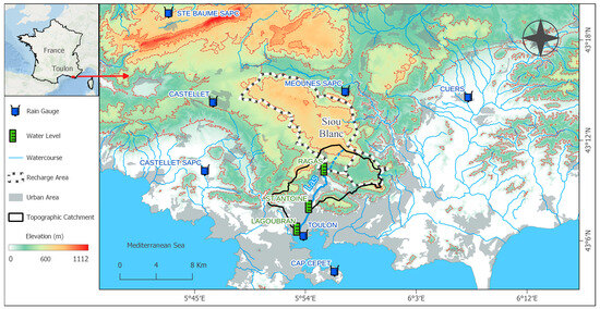
Figure 1.
Topography and streams of the Las basin (southeastern France), location of the water level gauging stations (Lagoubran at the Las River outlet in Toulon) and rain gauges. Data Sources: [14], (https://meteo.data.gouv.fr/, accessed on 31 January 2024), and (https://geoservices.ign.fr/bdtopo, accessed on 31 January 2024).
2.2. Database: Acquisition, Formatting, and Pre-Processing
Water level measurements at two springs feeding the river (Ragas and St Antoine) and at the river outlet (Lagoubran) are considered. The rainfall from seven stations located less than 10 km from the basin is also considered (Figure 1). The water level data were provided by [16,17] and cover the period from October 2012 to September 2018, with a 15 min time step. The rainfall data were downloaded from the French meteorological service (https://meteo.data.gouv.fr/ (accessed on 31 January 2024)), and cover the same period, with a 6 min time step. All data were resampled to a 15 min time step. To focus on flash flood events, periods with heavy rainfall were selected. We selected periods when the cumulative rainfall over 24 h exceeded 50 mm for at least one station. Missing rainfall values were supplemented by the average of the values from the most correlated rain gauges.
Correlograms between rainfall and water level at Lagoubran were calculated to determine the response time and the memory effect. The response time is defined as the time lag corresponding to the maximum of the correlogram. The memory effect is defined as the last time lag greater than the response time for which the correlation is higher than 0.2 [18]. The events defined from rainfall were classified in four categories based on the response time and the spring water level: quick urban runoff events, slow karst events, intermediate events, and events with low hydrological responses. Ref. [19] classified the rainfall events by karst water contributions and found similar events and classes. The present study only concerns the quick urban runoff events.
The event with the highest water level at Lagoubran (66% larger than the second one, 2.34 m vs. 1.41 m) was removed from the database to assess the model’s generalization capacity. It is referred to as the test event and was not used for the model’s training.
2.3. Model Design
This section explains the ANN’s design by detailing its structure, its input data, its training rule, and the criteria used to evaluate its performance. A set of the best hyperparameters was selected for AD on one hand, and LM on the other hand, to optimize the cross-validation score. This procedure maximizes the generalization properties of the models.
2.3.1. Input Dataset
The input dataset includes the rainfall time series at rain gauges over a sliding window of length , and the observed water level at Lagoubran over a sliding window of length 3 time steps. The output variable is the predicted water level at Lagoubran at a lead time of 2 time steps (30 min). The rainfall series with the best correlation with water level was used as input variables. Their sliding time windows (w) are their memory effect duration. The input dataset was normalized within the range 0–0.9.
2.3.2. Structure
The experiments were conducted using a fully connected multilayer perceptron with one hidden layer. Three hyperparameters were optimized: (1) the number of neurons, (2) the slope of the hidden layer’s activation function , and (3) the slope of the output layer’s activation function . The activation function of both layers is the hyperbolic tangent.
2.3.3. Parameter Initialization and Optimizers
Before the first epoch (iteration of training data), the weights of the ANN are initialized within a uniform distribution between −0.1 and 0.1, given a random seed. Biases are set to 0.1.
- Adam (AD): The learning rate of AD controls the pace of the update of the model’s parameters. It is crucial, as setting it too high may cause the loss function to oscillate between epochs and overshoot the global minimum, while setting it too low can result in slow and inefficient training [20]. The PyTorch 2.3.1 library’s [21] implementation of AD was used in this study. A learning rate of 0.1 with a maximum epoch of 100 showed that the loss function on the training dataset had a steady and smooth convergence curve with little fluctuations.
- Levenberg–Marquardt (LM): The damping parameter of LM controls the influence balance between the gradient descent contribution and the second-order contribution. It makes this algorithm react like a gradient descent algorithm at the start of training when the parameters are far from their optimal values, and like a second-order algorithm when the parameters are closer to their optimal values [22]. The LM algorithm is adapted from [9] and was implemented by [23]. As a rule of thumb, the damping parameter is 10−3 for LM, and its update factor is 0.1 if the loss function decreases and 10 if it increases. The maximum epoch used was 45.
2.3.4. Regularization Techniques
Regularization techniques prevent the ANN from overfitting on the training set and improve its performance and robustness on unseen events: the test set [11,24,25].
- Cross-validation splits the input dataset into event subsets. One subset is used as validation, while the others are in the training set. This is done for each event in a “leave-one event-out” manner [26], such that each event is used one time as validation. For each event, a score is calculated, and the average of all these scores is represented by the cross-validation score (CVS). The dataset is split by events to allow a clearer interpretation of the CVS.
- Early stopping stops the ANN’s training before full convergence [27]. An early stopping event is chosen disjointed to the cross-validation set. In a preliminary phase to the model selection, this set was chosen as the one that maximizes the cross-validation score; thus, this set is the most compatible with the learning set.
- The ensemble model increases the robustness of the optimized ANN model to the initial values of the parameters [5]. Ten ANNs were trained with different random sequences of initial parameters. The final output was the median of the results.
2.3.5. Performance Criteria
To evaluate the ANN’s performance, four metrics were used. All the criteria range from to 1. Here are the notations used for the criteria: is the discrete time, is the observed water level at , is the simulated water level at , is the lead time, is the time step where is maximum, and is the number of observations.
- Nash–Sutcliffe Efficiency (NSE) [28] (Equation (1)): it is used to measure the simulated variance error divided by the variance of the observed time series (here, the water level).
- Persistence coefficient (PERS) [29] (Equation (2)): it is similar to the NSE but adapted for predictions. When this criterion is positive, it indicates that the model’s output is better than the “naïve” forecast (the simplest forecast that assumes that the process value at the lead time is equal to the current value).
- Peak coefficient (PEAK) [30] (Equation (3)): It expresses the model’s ability to accurately simulate the water level at the time of the maximum observed peak.
- Combined criterion (PERS PEAK): It is the average of the PERS and PEAK, measuring the prediction’s ability of being both timely and reflecting accurately the peak values.
2.3.6. Model Selection
The rainfall series were ordered by decreasing maximum of cross-correlation with the observed water level. The first one was initially selected as a unique rainfall input to the model. Additional rainfall series were then added one by one to the ANN’s inputs, defining other input sets. For each input set, a hyperparameter grid search was carried out with the following hyperparameters: the number of hidden neurons (ranged from 1 to 15), (1, 3, 5), and (0.1, 0.5, 1). For each case, the model was trained and evaluated using the CVS. The model with the highest PERS PEAK CVS was selected for a wider analysis of its training and predictions. The performance of this model was evaluated on the test set. All operations used both optimization algorithms.
3. Results
3.1. Event Selection and Classification
The dataset contains 230,705 rainfall and water level observations after resampling of the rain gauge data on a 15 min time step. A total of 64 events were initially selected using the rainfall filter described in Section 2.3. However, only 49 were retained for classification due to missing water level data. These events were classified into four groups: 12 urban runoff events (representing 11,413 observations), 23 karst events, 7 intermediate events, and 7 low-water-level response events. The urban runoff events were characterized by faster response and memory effect times. Event 45 was used for early stopping and event 27 as the test event, and both were removed from the cross-validation events.
3.2. Model Selection on Urban Events
Based on the cross-correlation analysis between rainfall and water level, the rainfall series were ordered by maximum correlation: Castellet SAPC, Toulon, Cap Cepet, and Castellet; the corresponding response times are 11, 9, 11, and 11, respectively. These rainfall series were considered for the ANN inputs, with their corresponding memory effect as sliding windows (). The three other stations had lower correlations.
Figure 2 shows the cross validation scores of PERS PEAK for the AD and LM algorithms, for each rainfall series input set. It presents the CV score of the ANN for each hyperparameter set, as a function of its number of neurons. It appears that LM provides better scores. The LM scores show more variability when changing slopes than the AD scores.
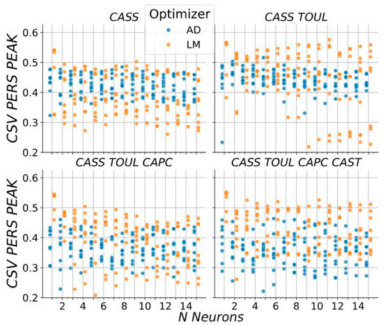
Figure 2.
Median of PERS PEAK criterion over cross-validation scores for all the models with different rainfall inputs; classified by the number of neurons and by the optimizer algorithms. Each point in this figure represents a set of slopes of the activation functions. Values lower than 0.2 are not shown. The input variables on the top are CASS: Castellet SAPC, TOUL: Toulon, CAPC: Cap Cepet, and CAST: Castellet.
Increasing decreased, on average, the performance of AD, while decreasing improved the performance of LM. Other experiments not highlighted in the methodology showed that logistic sigmoid activation functions performed worse than the hyperbolic tangent. Regarding the computation time, LM took on average 5 times more time during training, despite using a lower maximum number of iterations of 30 for LM and 100 for AD. As the number of neurons increases, the difference in the training duration between the optimizers increases. The lower training duration of AD within experiences is probably accentuated by the optimizations of the native PyTorch 2.3.1 AD optimizers.
The selection of hyperparameters and inputs led to the best models having Castellet SAPC and Toulon as inputs and AD with 5 neurons, of 3 and of 0.1, and LM with 11 neurons, of 1 and of 0.1. These architectures performed similarly on the cross-validation events with a median NSE of 0.69 for AD vs. 0.702 for LM, and a median PERS PEAK of 0.516 for AD vs. 0.576 for LM. During training, the loss function was lower for LM compared to AD. LM fits the training set better with fewer epochs, 20 at most. LM requires an early stopping set to prevent overfitting, while AD does not overfit the training set with an optimal learning rate and thus does not require an early stopping set. The PERS PEAK of AD improved by a factor of 3 when training was stopped over 100 epochs.
3.3. Predictions on Test Event
The test event was an exceptional event with 123% and 147% higher maximum rainfall intensity, respectively, at Castellet SAPC and Toulon than in the cross-validation events. This caused the water level to rise 66% above the records in the cross-validation events. All the criteria used showed an approximate 0.25 increase in the predictions of the test event with LM compared to AD (Figure 3). These results show that LM can better generalize extreme and unprecedented events.
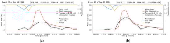
Figure 3.
Hydrograph showing test event observations and predictions at + 30 min for the best model with (a) AD and (b) LM optimizers. The black curve represents the median of the 10 grey curves, each corresponding to a model with a different parameter initialization.
Furthermore, training the same model with LM over 30 epochs improved by 0.27 the prediction PEAK of the test event, suggesting that predicting extreme events requires an extended training of the ANN (Figure 4). This was not observed for AD.
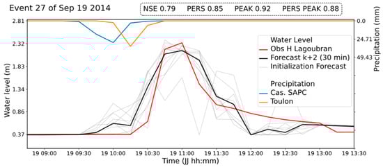
Figure 4.
Hydrograph showing test event observations and predictions at + 30 min for the best model with the LM optimizer at 30 epochs.
4. Discussion
The rainfall water level cross-correlation analysis revealed that the highest correlation was related to the Castellet SAPC station, 13 km northwest of the Lagoubran water level station. As this station is located on the first hill slopes (66 m above sea level), its rains may be representative of the orographic uplift of maritime winds. This shows that the rainfall stations closest to the target station are not always the best correlated ones. This suggests that the choice of stations could be improved by using cross-validation during the model selection rather than cross-correlation.
The convergence of AD is highly dependent on the value of its learning rate, while LM does not have such a parameter. The damping parameter of LM ensures the ANN’s convergence in a clever way. LM requires an early stopping set because it fits more to the training set compared to AD. When a stop event is used with AD, it stops learning too early, even before the cost function has converged.
Regarding the ability to forecast extreme event 27 (of 19 September 2014), it is clear (Figure 3 and Figure 4) that it is well modeled under the condition of adding more epochs to the training. This shows that the LM optimizer is able to reproduce this extreme event (66% bigger than the second-biggest event in the database), but not yet automatically (in a blind test). This ability has not been demonstrated by AD. Despite the LM optimizer having a higher computational cost than AD during training, the operational computational cost of operations remains the same, with low resource requirements and fast prediction times. Furthermore, there are promising methods to improve the memory and time efficiencies of the LM algorithm, such as computing directly the quasi-Hessian matrix with the gradient vector without the Jacobian [31] or addressing the minimization algorithm [32].
A common example of LM outperforming AD is when fitting a simple sinc function with a variable amplitude and a constant frequency using a shallow network [12,23]. In contrast to the results of the study, where higher amplitudes were better predicted with LM, AD fails to converge with a bad fit of lower amplitudes while having a good fit of higher amplitudes in Taylor’s experiments.
5. Conclusions
This study focuses on extreme flash flood forecasting using an ANN with AD and LM optimization algorithms. Both optimizers were set to their best training conditions. The ANN’s inputs were selected by linear cross-correlation analysis of rainfall and water level time series. A hyperparameter grid search was performed to select the model with the timeliest predictions and accurate peak values on urban runoff events. The performance during training and prediction of the best AD and LM models was compared.
LM benefited from the early stopping regularization technique because it usually overfits the training set, while AD had an earlier stop. LM outperformed AD in CVS on the hyperparameter selection, and the PERS PEAK CVS of the best models was 0. 516 for AD versus 0.576 for LM. During the ANN’s training, the loss function of LM converged with fewer epochs compared to AD. On the test event, where the water level was 66% higher than in all events considered for training, LM forecasts were improved by 0.25 compared to AD. There is ways for improvement in terms of learning stop, which could potentially lead to further improvement in the performance of the Levenberg Marquardt rule, resulting in a near-perfect forecast of the most intense event in the database. The main shortcoming of LM compared to AD is that its training time is 5 times longer than that of the AD algorithm. Further investigation needs to be conducted to define the most appropriate early stopping criteria for enabling LM to predict extreme unseen events.
To confirm the conclusions of this study, it is necessary to reproduce the methodology in other study areas, with more diverse datasets. Only ANNs in the structure of shallow multilayer perceptrons were used in this study; it could be interesting to investigate other ANN structures, such as LSTMs or transformers, to assess the potential benefits in relation to the significant increase in complexity.
Author Contributions
Conceptualization, methodology, formal analysis, J.Y.P.A., V.W., A.J., A.D., B.A. and S.P.; methodology, J.Y.P.A., V.W., A.J., A.D. and S.P.; software, validation, visualization, and writing—original draft preparation J.Y.P.A., V.W., B.A. and A.J.; investigation, resources, data curation, writing—review and editing, all authors; supervision, V.W., A.J., A.D. and S.P.; project, J.Y.P.A., A.J., G.A., A.D., B.A. and S.P. All authors have read and agreed to the published version of the manuscript.
Funding
This research was funded by the French National Research Agency (ANR-21-LCV1-0001) as part of the “Hydrological Forecasting Laboratory Using Artificial Intelligence” (Hydr.IA) project.
Data Availability Statement
The data used and generated for this article will be made available by the authors upon request.
Acknowledgments
We are grateful to the ANR for funding this research, to Météo-France for the availability of rain gauge data, and to Synapse Informatique company for their collaboration in this project. We thank the reviewers for their constructive feedback.
Conflicts of Interest
The authors declare no conflicts of interest.
References
- Funahashi, K.-I. On the Approximate Realization of Continuous Mappings by Neural Networks. Neural Netw. 1989, 2, 183–192. [Google Scholar] [CrossRef]
- Barron, A.R. Universal Approximation Bounds for Superpositions of a Sigmoidal Function. IEEE Trans. Inf. Theory 1993, 39, 930–945. [Google Scholar] [CrossRef]
- Shen, C. A Transdisciplinary Review of Deep Learning Research and Its Relevance for Water Resources Scientists. Water Resour. Res. 2018, 54, 8558–8593. [Google Scholar] [CrossRef]
- Kong A Siou, L.; Johannet, A.; Borrell, V.; Pistre, S. Complexity Selection of a Neural Network Model for Karst Flood Forecasting: The Case of the Lez Basin (Southern France). J. Hydrol. 2011, 403, 367–380. [Google Scholar] [CrossRef]
- Darras, T.; Johannet, A.; Vayssade, B.; Kong-A-Siou, L.; Pistre, S. Ensemble Model to Enhance Robustness of Flash Flood Forecasting Using an Artificial Neural Network: Case-Study on the Gardon Basin (South-Eastern France). Bol. Geol. Y Min. 2018, 129, 565–578. [Google Scholar] [CrossRef]
- Tan, H.H.; Lim, K.H. Review of Second-Order Optimization Techniques in Artificial Neural Networks Backpropagation. Proc. IOP Conf. Ser. Mater. Sci. Eng. 2019, 495, 12003. [Google Scholar] [CrossRef]
- Kingma, D.P. Adam: A Method for Stochastic Optimization. arXiv 2014, arXiv:1412.6980. [Google Scholar]
- Levenberg, K. A Method for the Solution of Certain Non-Linear Problems in Least Squares. Q. Appl. Math. 1944, 2, 164–168. [Google Scholar] [CrossRef]
- Marquardt, D.W. An Algorithm for Least-Squares Estimation of Nonlinear Parameters. J. Soc. Ind. Appl. Math. 1963, 11, 431–441. [Google Scholar] [CrossRef]
- Ranganathan, A. The Levenberg-Marquardt Algorithm. Tutoral LM Algorithm 2004, 11, 101–110. [Google Scholar]
- Maier, H.R.; Dandy, G.C. Neural Networks for the Prediction and Forecasting of Water Resources Variables: A Review of Modelling Issues and Applications. Environ. Model. Softw. 2000, 15, 101–124. [Google Scholar] [CrossRef]
- Taylor, J.; Wang, W.; Bala, B.; Bednarz, T. Optimizing the Optimizer for Data Driven Deep Neural Networks and Physics Informed Neural Networks. arXiv 2022, arXiv:2205.07430. [Google Scholar] [CrossRef]
- Gaume, E.; Borga, M.; Llassat, M.C.; Maouche, S.; Lang, M.; Diakakis, M. Mediterranean Extreme Floods and Flash Floods. In The Mediterranean Region Under Climate Change. A Scientific Update; Coll. Synthèses; IRD Editions: 1313; pp. 133–144. Available online: https://hal.inrae.fr/hal-02605195v1 (accessed on 22 July 2025).
- Baudement, C.; Arfib, B.; Mazzilli, N.; Jouves, J.; Lamarque, T.; Guglielmi, Y. Groundwater Management of a Highly Dynamic Karst by Assessing Baseflow and Quickflow with a Rainfall-Discharge Model (Dardennes Springs, SE France). BSGF-Earth Sci. Bull. 2017, 188, 40. [Google Scholar] [CrossRef]
- Insee Populations Légales 2021 Recensement de La Population Régions, Départements, Arrondissements, Cantons et Communes 2021. Web reference. Available online: https://www.insee.fr/fr/statistiques/zones/7725600?geo=COM-83137&debut=0 (accessed on 22 July 2025).
- SNO KARST. Time Series of Type Hydrology-Hydrogeology in Dardennes—Le Las Basin—PORT-MIOU Observatory—KARST Observatory Network—OZCAR Critical Zone Network Research Infrastructure. OSU OREME. 2024. Available online: https://www.data.gouv.fr/datasets/66d10c9e1965f267407093b1/ (accessed on 22 July 2025).
- Dufresne, C.; Arfib, B.; Ducros, L.; Duffa, C.; Giner, F.; Rey, V.; Lamarque, T. Datasets of Solid and Liquid Discharges of an Urban Mediterranean River and Its Karst Springs (Las River, SE France). Data Brief 2020, 31, 106022. [Google Scholar] [CrossRef]
- Mangin, A. Pour Une Meilleure Connaissance Des Systèmes Hydrologiques à Partir Des Analyses Corrélatoire et Spectrale. J. Hydrol. 1984, 67, 25–43. [Google Scholar] [CrossRef]
- Dufresne, C.; Arfib, B.; Ducros, L.; Duffa, C.; Giner, F.; Rey, V. Karst and Urban Flood-Induced Solid Discharges in Mediterranean Coastal Rivers: The Case Study of Las River (SE France). J. Hydrol. 2020, 590, 125194. [Google Scholar] [CrossRef]
- Reddi, S.J.; Kale, S.; Kumar, S. On the Convergence of Adam and Beyond. arXiv 2019, arXiv:1904.09237. [Google Scholar] [CrossRef]
- Paszke, A.; Gross, S.; Massa, F.; Lerer, A.; Bradbury, J.; Chanan, G.; Killeen, T.; Lin, Z.; Gimelshein, N.; Antiga, L.; et al. Pytorch: An Imperative Style, High-Performance Deep Learning Library. Adv. Neural Inf. Process Syst. 2019, 32. Available online: https://arxiv.org/abs/1912.01703 (accessed on 22 July 2025).
- Gavin, H.P. The Levenberg-Marquardt Algorithm for Nonlinear Least Squares Curve-Fitting Problems. Department of Civil and Environmental Engineering Duke University August 2019. Volume 3. Available online: https://people.duke.edu/~hpgavin/ExperimentalSystems/lm.pdf (accessed on 22 July 2025).
- Di Marco, F. Torch-Levenberg-Marquardt. GitHub Repository 2025. Available online: https://github.com/fabiodimarco/torch-levenberg-marquardt (accessed on 22 July 2025).
- Geman, S.; Bienenstock, E.; Doursat, R. Neural Networks and the Bias/Variance Dilemma. Neural Comput. 1992, 4, 1–58. [Google Scholar] [CrossRef]
- Kong A Siou, L.; Johannet, A.; Valérie, B.E.; Pistre, S. Optimization of the Generalization Capability for Rainfall–Runoff Modeling by Neural Networks: The Case of the Lez Aquifer (Southern France). Environ. Earth Sci. 2012, 65, 2365–2375. [Google Scholar] [CrossRef]
- Stone, M. Cross-Validatory Choice and Assessment of Statistical Predictions. J. R. Stat. Soc. Ser. B (Methodol.) 1974, 36, 111–133. [Google Scholar] [CrossRef]
- Amari, S.; Murata, N.; Muller, K.-R.; Finke, M.; Yang, H.H. Asymptotic Statistical Theory of Overtraining and Cross-Validation. IEEE Trans. Neural Netw. 1997, 8, 985–996. [Google Scholar] [CrossRef]
- Nash, J.E.; Sutcliffe, J. V River Flow Forecasting through Conceptual Models Part I—A Discussion of Principles. J. Hydrol. 1970, 10, 282–290. [Google Scholar] [CrossRef]
- Kitanidis, P.K.; Bras, R.L. Real-Time Forecasting with a Conceptual Hydrologic Model: 2. Applications and Results. Water Resour. Res. 1980, 16, 1034–1044. [Google Scholar] [CrossRef]
- Artigue, G.; Johannet, A.; Borrell, V.; Pistre, S. Flash Flood Forecasting in Poorly Gauged Basins Using Neural Networks: Case Study of the Gardon de Mialet Basin (Southern France). Nat. Hazards Earth Syst. Sci. 2012, 12, 3307–3324. [Google Scholar] [CrossRef]
- Wilamowski, B.M.; Yu, H. Improved Computation for Levenberg–Marquardt Training. IEEE Trans. Neural Netw. 2010, 21, 930–937. [Google Scholar] [CrossRef] [PubMed]
- Finsterle, S.; Kowalsky, M.B. A Truncated Levenberg–Marquardt Algorithm for the Calibration of Highly Parameterized Nonlinear Models. Comput. Geosci. 2011, 37, 731–738. [Google Scholar] [CrossRef]


Disclaimer/Publisher’s Note: The statements, opinions and data contained in all publications are solely those of the individual author(s) and contributor(s) and not of MDPI and/or the editor(s). MDPI and/or the editor(s) disclaim responsibility for any injury to people or property resulting from any ideas, methods, instructions or products referred to in the content. |
© 2025 by the authors. Licensee MDPI, Basel, Switzerland. This article is an open access article distributed under the terms and conditions of the Creative Commons Attribution (CC BY) license (https://creativecommons.org/licenses/by/4.0/).