Statistical Machine Learning Approaches to Liver Disease Prediction

Abstract

Medical diagnoses have important implications for improving patient care, research, and policy. For a medical diagnosis, health professionals use different kinds of pathological methods to make decisions on medical reports in terms of the patients’ medical conditions. Recently, clinicians have been actively engaged in improving medical diagnoses. The use of artificial intelligence and machine learning in combination with clinical findings has further improved disease detection. In the modern era, with the advantage of computers and technologies, one can collect data and visualize many hidden outcomes such as dealing with missing data in medical research. Statistical machine learning algorithms based on specific problems can assist one to make decisions. Machine learning (ML), data-driven algorithms can be utilized to validate existing methods and help researchers to make potential new decisions. The purpose of this study was to extract significant predictors for liver disease from the medical analysis of 615 humans using ML algorithms. Data visualizations were implemented to reveal significant findings such as missing values. Multiple imputations by chained equations (MICEs) were applied to generate missing data points, and principal component analysis (PCA) was used to reduce the dimensionality. Variable importance ranking using the Gini index was implemented to verify significant predictors obtained from the PCA. Training data ($n_{train}=399$) for learning and testing data ($n_{test}=216$) in the ML methods were used for predicting classifications. The study compared binary classifier machine learning algorithms (i.e., artificial neural network, random forest (RF), and support vector machine), which were utilized on a published liver disease data set to classify individuals with liver diseases, which will allow health professionals to make a better diagnosis. The synthetic minority oversampling technique was applied to oversample the minority class to regulate overfitting problems. The RF significantly contributed ($p<0.001$) to a higher accuracy score of 98.14% compared to the other methods. Thus, this suggests that ML methods predict liver disease by incorporating the risk factors, which may improve the inference-based diagnosis of patients.

1. Introduction

To detect disease, healthcare professionals need to collect samples from patients which can cost both time and money. Often, more than one kind of test or many samples are needed from the patient to accumulate all the necessary information for a better diagnosis. The most routine tests are urinalysis, complete blood count (CBC), and comprehensive metabolic panel (CMP). These tests are generally less expensive and can still be very informative.

The liver has many functions such as glucose synthesis and storage, detoxification, production of digestive enzymes, erythrocyte regulation, protein synthesis, and various other features of metabolism. Chronic liver diseases include chronic hepatitis, fibrosis, and cirrhosis. Hepatitis can occur from viral infection (e.g., hepatitis c virus) or auto-immune origin. Inflammation from hepatitis infection can cause tissue damage and scarring to occur in the liver. Moderate scarring is classified as fibrosis, while severe liver damage/scarring is classified as cirrhosis. Fibrosis and cirrhosis can also occur from alcoholism and non-alcoholic fatty liver disease. When liver disease is diagnosed at an earlier stage, in between infection and fibrosis but before cirrhosis, liver failure can be avoided. Tests, such as a CMP and biopsy, can be conducted to diagnose all forms of liver disease. A CMP with a liver function panel can detect albumin (ALB), alkaline phosphatase (ALP), alanine amino-transferase (ALT), aspartate amino-transferase (AST), gamma glutamyl-transferase (GGT), creatine (CREA), total protein (PROT), and bilirubin (BIL). Diagnosis of a certain liver disease and discovery of its origin are made by interpreting the patterns and ratios of circulating liver-associated molecules measured with the CMP test and compared to values normalized with a patient’s age, sex, and BMI. Aminotransferases, AST, and ALT are enzymes that participate in gluconeogenesis by catalyzing the reaction of transferring alpha-amino groups to ketoglutaric acid groups. AST is found in many tissue types and is not as specific to the liver but may denote secondary non-hepatic causes of liver malfunction. ALT is found in high concentrations in the cytosol of liver cells. Liver cell injury can cause the release of both aminotransferases into circulation. When ALT is significantly increased in proportion to ALP, the liver disease is likely from an inflammatory origin (acute or chronic viral hepatitis and autoimmune disease) [1]. Higher levels of AST than ALT can mean alcoholic liver disease [2]. When ALT and AST are increased equally, fatty liver or non-alcoholic liver disease may be the case [3]. ALP consists of a family of zinc metalloproteases that catalyze hydrolysis of organic phosphate esters. ALP in circulation is most likely from liver, bone, or intestinal origin. Mild to moderate elevation of ALP can reflect hepatitis and cirrhosis, but these results are less specific unless confirmed by liver-specific enzymes such as GGT [4]. A substantial increase in ALP is correlated with biliary tract obstruction, as concentrations of ALP increase in cells closer to the bile duct [5]. GGT is found in membranes of highly secretory cells such as the liver [6]. Heme catabolism from hemoglobin produces BIL, which is conjugated to bilirubin glucuronide in the liver to be secreted with bile, a substance produced by the liver to expedite digestion. Unconjugated BIL is bound to ALB for transport to the liver in order for it to be conjugated. ALB is synthesized exclusively in the liver and can be used as a marker for hepatic synthetic activity. Chronic disease of the liver can result in decreased concentration of serum ALB, while more acute cases likely will not cause this dip in ALB [7].

Liver-related disease accounts for 70% of deaths worldwide [8]. There is a need to find better ways to detect and diagnose liver disease with more accuracy. Most importantly, tests of liver function need to be available and affordable to patients. To avoid the expensive and invasive tests, the application of statistical machine learning techniques to CMP results for the extraction of information for a clinician might be helpful for diagnosis [7,9]. Exploratory data analysis methods are extremely important in healthcare; they can predict patterns across data sets to facilitate the determination of risk or diagnostic factors for disease with more speed and accuracy. The use of these methods can allow for earlier detection and potentially prevent many cases of liver disease from progressing to the point of needing biopsy or complex treatment.

ML algorithms are new techniques to handle many hidden problems in medical data sets. This approach can help healthcare management and professionals to explore better results in numerous clinical applications, such as medical image processing, language processing, and tumor or cancer cell detection, by finding appropriate features. Several statistical and machine learning approaches (e.g., simulation modeling, classification, and inference) have been used by researchers and lab technicians for better prediction [10,11,12,13]. The clinical results are more data-driven than model-dependent. In medical diagnosis, finding the appropriate target (response variable) [14] and features are very challenging for classification problems. Logistic regression is a widely used technique, but its performance is relatively poorer than several machine learning and deep learning methods [15,16,17]. First of all, data visualization is necessary to understand latent knowledge about predictors, which is a part of exploratory data analysis [18]. Among many techniques, the whisker plot indicates variability outside the upper and lower quantiles, which are known as outliers. Another common problem in real-life application of data science is missing values in a data set. Missing data are a continuous problem in medical research, arising from various causes such as participants dropping out of studies or laboratory technician errors. Missing data lower the statistical power and could introduce bias into medical studies [19]. Many methods have been tried to solve this problem. However, the wrong imputation of missing values can lead models toward the wrong prediction. MICE is known as multiple imputation by chained equations which helps to manipulate missing variables [20,21]. It gives the assumption of missing data at a random procedure which is investigated as the missing at random (MAR) method. MAR implies that the probability of a missing value depends only on observed values, not the values that are not observed [22]. This procedure creates numerous predictions for each missing value with multiple imputed data taking into consideration uncertainty in the imputations and produces some accurate standard errors. The MICE algorithm [23,24] is a good performer among many of the data imputation methods. A heatmap is another way to see the correlation between input and output variables [25]. Moreover, medical disease detection mostly relies on biological and biochemical markers, where all of them are not significant for diagnosis. For optimal biomarker selection, PCA is a conventional technique to reduce dimensionality in medical diagnosis [26]. Many researchers from different fields have studied binary classification using machine learning [15] for detecting breast cancer, skin cancer, and many other problems related to disease prognosis. For example, Hoffmann et al. [27] used decision tree algorithms for classification. Moreover, one of the used methods is the support vector machine [28], which was introduced by Boser, Guyon, and Vapnik in COLT-92 [29]. It helps to divide the label by the hypersphere of a linear function in a high-dimensional feature space, which was developed with a learning algorithm from mathematical optimization, where the learning bias will be calculated using statistical learning. SVM assists in making decisions using maximum linear classifiers with the highest range [30]. The improved SVM classifier, based on the improvement of a trade-off between margin and radius, was studied by Rizwan et al. [31]. Another model for classification problems is the ANN, which is similar to neurons in human health. Machine learning for breast cancer detection with ANN was studied by Jafari-Marandi et al. [28]. Another method that outperforms decision tree algorithms is called RF [32,33], which is used to predict classification. ML procedures have been studied by many researchers for binary classification of cancer data and X-ray image data for pattern recognition [24,33]. Pianykh et al. [34] studied healthcare operation management using machine learning.

Literature Review

Using machine learning algorithms to predict disease is made possible by increasing access to hidden attributes in medical data sets. Various kinds of data sets, such as blood panels with liver function tests, histologically stained slide images, and the presence of specific molecular markers in blood or tissue samples, have been used to train classifier algorithms to predict liver disease with good accuracy. The ML methods described in previous studies have been evaluated for accuracy by a combination of confusion matrix, receiver operating characteristic under area under curve, and k-fold cross-validation. Singh et al. designed software based on classification algorithms (including logistic regression, random forest, and naive Bayes) to predict the risk of liver disease from a data set with liver function test results [35]. Vijayarani and Dhavanand found that SVM performed better over naive Bayes to predict cirrhosis, acute hepatitis, chronic hepatitis, and liver cancers from patient liver function test results [36]. SVM with particle swarm optimization (PSO) predicted the most important features for liver disease detection with the highest accuracy over SVM, random forest, Bayesian network, and an MLP-neural network [37]. SVM more accurately predicted drug-induced hepatotoxicity with reduced molecular descriptors than Bayesian and other previously used models [38]. Phan and Chan et al. demonstrated that a convolutional neural network (CNN) model predicted liver cancer in subjects with hepatitis with an accuracy of 0.980 [39]. The ANN model has been used to predict liver cancer in patients with type 2 diabetes [40]. Neural network ML methods can help differentiate between types of liver cancers when applied to imaging data sets [41]. Neural network algorithms have even been trained to predict a patient’s survival after liver tumor removal using a data set containing images of processed and stained tissue from biopsies [42]. ML methods can facilitate the diagnosis of many diseases in clinical settings if trained and tested thoroughly. More widespread application of these methods to varying data sets can further improve accuracy in current deep learning methods.

This study aimed to (i) impute missing data using the MICE algorithm; (ii) determine variable selection using eigen decomposition of a data matrix by PCA and to rank the important variables using the Gini index; (iii) compare among several statistical learning methods the ability to predict binary classifications of liver disease; (iv) use the synthetic minority oversampling technique (SMOTE) to oversample minority class to regulate overfitting; (v) obtain confusion matrices for comparing actual classes with predictive classes; (vi) compare several ML approaches to assess a better performance of liver disease diagnosis; (viii) evaluate receiver operating characteristic (ROC) curves for determining the diagnostic ability of binary classification of liver disease.

2. Materials and Methods

2.1. Data Description

Data were collected from the University of California Irvine Machine Learning Repository. The data set was included with laboratory reports of blood donors and non-blood donors with Hepatitis C and demographic information such as age and sex. The response variable for classification was categorical variable: healthy individuals (i.e., blood donors) vs. patients with liver disease (i.e., non-blood donors) including its progress, e.g., hepatitis C, fibrosis, and cirrhosis. The data set contained 14 attributes such as ALB, ALP, BIL, choline esterase (CHE), GGT, AST, ALT, CREA, PROT, and cholesterol (CHOL). The sex and outcome variables were categorical, and the age variable was continuous. Hoffmann et al. [27] used machine learning algorithms to validate existing or to suggest potentially new decision trees using a subset of the same data set. They compared two machine learning algorithms that automatically generate decision trees from real-life laboratory data related to liver fibrosis and cirrhosis in patients with chronic hepatitis C infection. They used 73 patients (52 males, 21 females) with a proven serological and histopathological diagnosis of hepatitis C. The present study used 615 patients’ data (376 males, 239 females).

2.2. Definition of Variables

The variables were found through comprehensive metabolic panel and liver function panel results using patient blood samples. Most variables were measured in g/L.

Albumin: a protein synthesized exclusively by the liver, indicative of hepatic synthetic ability;

Alkaline phosphatase: a family of zinc metalloproteases that catalyze hydrolysis of organic phosphate esters;

Bilirubin: end product of hemoglobin catabolism, secreted by the liver with bile after it is conjugated, which occurs in the liver and spleen;

Choline esterase: a group of enzymes that hydrolyze esters in choline;

Gamma glutamyl-transferase: An enzyme that catalyzes the transfer of gamma-glutamyl groups of peptides to other amino acids or peptides. Serum GGT is derived mostly from the liver;

Aspartate aminotransferase: Aminotransferase that catalyzes the transfer of the alpha-amino group from aspartate to the alpha-keto group of ketogluric acid, creating oxaloacetic acid. It is important for the diagnosis of hepatocellular injury;

Alanine aminotransferase: aminotransferase that catalyzes the transfer of the alpha-amino group from alanine to the alpha-keto group of ketogluric acid, creating pyruvic acid. It is important for the diagnosis of hepatocellular injury.

Creatinine: waste product of metabolism, usually filtered out and excreted by kidneys through urine;

Total protein: Total protein in the blood. Measurement of two main protein types found in circulation, albumin and globulin, and;

Cholesterol: Measurement of total cholesterol in the blood; HDL and LDL are the main lipids identified. This can detect risks for heart disease or stroke.

2.3. Sample Size and Power Calculation

The total data contained sociodemographic and biochemical variables of 615 patients. The sample size was calculated using G*Power software (version 3.1.9.4) [43]. A total of 88 subjects were sufficient to detect a statistically significant relationship between categorical variables with a 5% level of significance, median effect size = 0.30, and power = 80% when running a chi-squared test. In general, males are 2-fold more likely to die from chronic liver disease and cirrhosis than females [8]. Furthermore, it was determined that 201 subjects were required for logistic regression analysis based on 61% males (376) with liver disease, 39% females (239) with liver disease, alpha (α) = 0.05, power = 80%, and a two-sided testing procedure. The study sample was large enough for statistical analysis.

2.4. Study Design

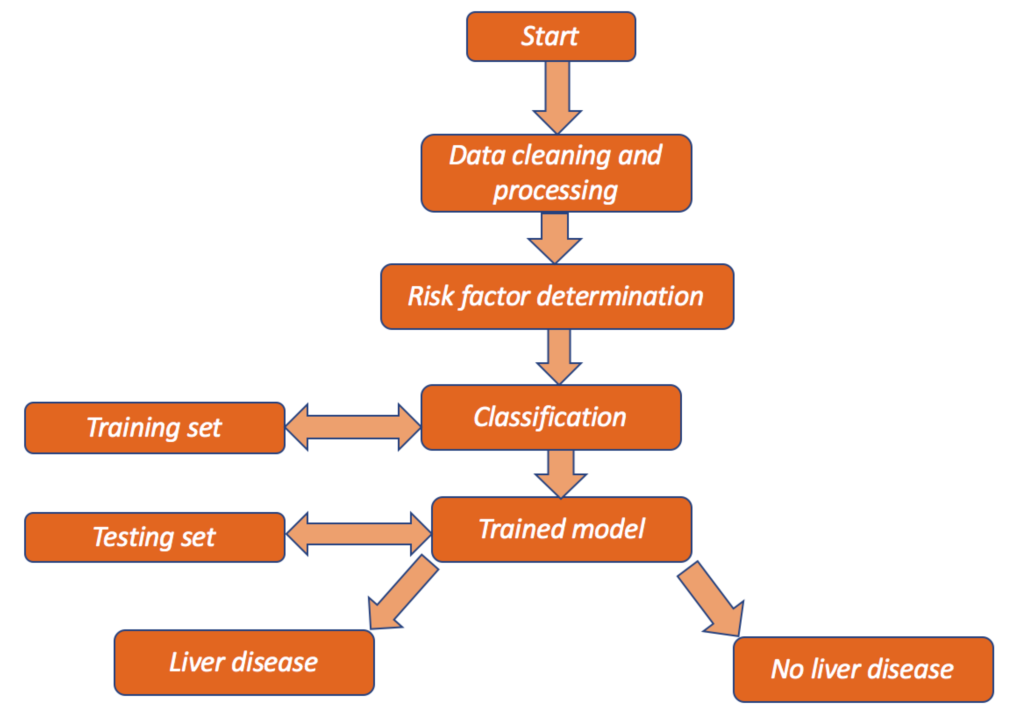
A flow chart is presented in Figure 1 below to show the overview of the design of the study.

2.5. Data Visualization and Target Labeling

Missing data are quite a common scenario in the application of data science. In this study, data were investigated using different plots to detect groups of individuals who had liver disease and no liver disease. The target variable was modified into a binary category, labeled “0” for no liver disease and “1” for liver disease. The following method was used to fill out missing data for each predictor in the multivariate data. The missing values are needed to impute so that the data set remains in balance and to obtain a better estimation of prediction.

2.6. Multiple Imputation by Chained Equations for Missing Data

Multiple imputation was used via the chained equations method to generate the missing data. For multivariate missing data, the R-package [22] known as “MICE” was used for multiple imputations. This function auto-detects certain variables with missing values. It basically uses predictive mean matching (PMM), which is a semi-parametric imputation. It is very close to regression except missing items are randomly filled by regression prediction. The algorithms for MICE are given below.

Step 1: Start with imputing the mean. Mean imputations are considered “position holders”;

Step 2: the “position holder” presents imputations for one variable (“Var”) which are impeded to the missing items;

Step 3: “Var” is the response variable where the other variables are predictor variables in the linear regression model (under the same assumption);

Step 4: the missing values for “Var” are then replaced with imputed values from the regression model;

Step 5: Repeat steps 2–4 and produce the missing data. One iteration is needed for each variable and, finally, the missing values. Ten such cycles were performed by Raghunathan et. al. [21].

Exploratory data analysis is used to determine the hidden attributes of a data set. Examples of exploratory methods are correlation heatmaps and box plots to help visualize the data [39]. One of the main goals of this study was to determine the most important metrices that describe almost all of the data set but, at the same time, keeps the loss of information to a minimum. The need for multiple tests per patient increases the cost associated with liver disease but may be required for accuracy in diagnosis. Reducing the dimensions can be helpful for clinicians to determine which biochemical markers are most important for diagnosis and pattern evaluation, therefore, reducing the number of tests for patients in the future. Statistical learning methods, such as PCA, assist in reducing the dimensionality of a data set.

2.7. Principal Component Analysis for Dimension Reduction

Let $\mathit{X}\in R^{n\times p}$ be the data matrix with the integer $k (\mathrm{with} 0<k<p)$. PCA [26] can be determined through singular value decomposition (SVD). For this, let $\mathit{X}={\left(x_1^T,x_2^T,\dots ,x_n^T\right)}^T$ and $\tilde{\mathit{X}}={\left({\tilde{x}}_1^T,{\tilde{x}}_2^T,\dots ,{\tilde{x}}_n^T\right)}^T\in R^{n\times p} \left(\mathrm{where} {\tilde{x}}_i=x_i-\overline{x}\right)$ be the original and centered data matrices, respectively. Then, the square matrix $\mathit{C}$ is a symmetric and positive semidefinite, which is defined as follows:

$$\mathit{C}={\displaystyle \sum }{\tilde{x}}_i{\tilde{x}}_i{}^T=\left[{\tilde{x}}_1^T,{\tilde{x}}_2^T,\dots ,{\tilde{x}}_n^T\right]{\left[{\tilde{x}}_1^T,{\tilde{x}}_2^T,\dots ,{\tilde{x}}_n^T\right]}^T={\tilde{\mathit{X}}}^T\tilde{\mathit{X}}.$$

(1)

The principal direction of the data set is given by the top eigenvectors for the corresponding eigenvalues of the covariance matrix. Thus, the dimension of $\mathit{C} \mathrm{is} p\times p$. More mathematically, it is the right singular vector of $\tilde{\mathit{X}}:$

$${\tilde{\mathit{X}}}^{\mathit{T}}\tilde{\mathit{X}}=\mathit{V}{\Sigma }^{\mathit{T}}{\mathit{U}}^{\mathit{T}}\mathit{U}\Sigma {\mathit{V}}^{\mathit{T}}=\mathit{V}\left(\Sigma {\Sigma }^{\mathit{T}}\right){\mathit{V}}^{\mathit{T}},$$

(2)

where columns of $\mathit{V}$ are the principal directions, $\Sigma$ is the singular values, where ${\lambda }_i={\sigma }_i^2$ is the eigenvalue by each principal direction, and columns of $\mathit{U}\Sigma$ are different principal components of the data set $\mathit{X}$.

2.8. Training and Testing Data

According to statistical machine learning techniques, the data set collected from Hoffmann et al. [39] was divided into training and testing data sets, where the training set was applied to fit the parameters. A part of training set was used for validation (see Figure 2). In fact, it was split into training and test data sets based on 5-fold cross-validation on the mis-classification error.

In this study, several binary classification techniques were applied. All of them are discussed briefly. Classification methods were applied to the reduced data set with the PCA and Gini index selected risk factors. Training data ($n_{train}=399$) for learning and testing data ($n_{test}=216$) for testing were obtained by simple random sampling techniques. Train data were used to train the ML classification methods for predicting binary classifications. Finally, a confusion matrix is shown using the test data set. In the next subsection, ML binary classification methods are discussed briefly.

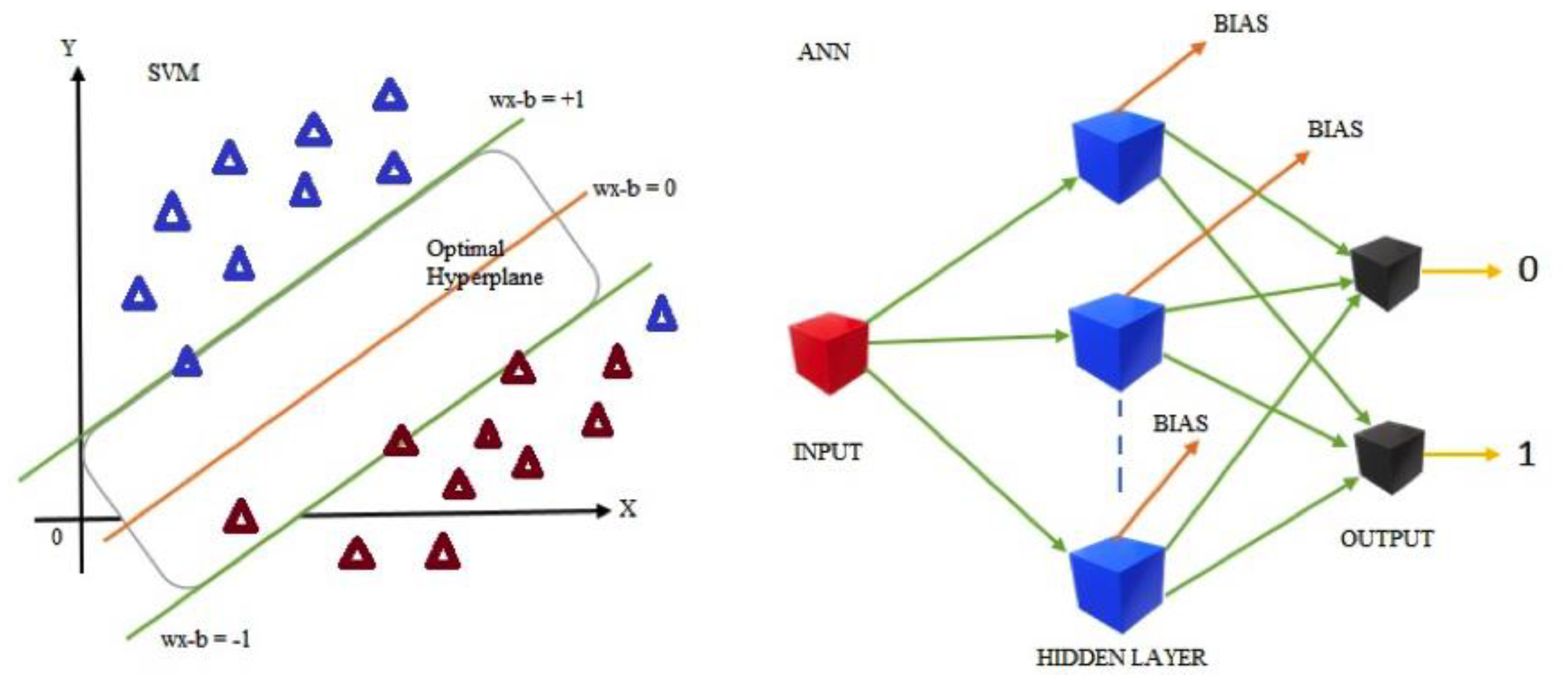
2.9. Support Vector Machine Classification

SVM [29,30,31,32] is a linear classifier that determines the maximum hyperplane separation margin. SVM’s purpose is to partition data sets into classes so that a maximum marginal hyperplane can be found (MMH) [32]. Since the categorical target variable is binary in nature, it was labeled as 0 for no liver disease and 1 for liver disease. Thus, SVM [34] works by following two steps:

Step 1: SVM iteratively constructs hyperplanes that best separate the classes;

Step 2: the hyperplane that correctly separates the classes are then chosen.

The training data set has $n_{train}$ data points from original data set $\left(x_1,y_1\right),\dots ,\left(x_n,y_n\right)$, where $y_i$ is either $+1$ or $-1$, each including a label to the point $x_i$. Each $x_i$ is a $p$ dimensional real vector. A maximum margin hyperplane divides the group of points of $x_i$ for which the target variable can be defined as follows:

$$y_i=\{\begin{array}{l}+1\\ -1,\end{array}$$

where $-1$ is considered 0 and $+1$ as 1. SVM is a hyperplane classifier, and the mathematical equation of hyperplane can be either positive or negative. The classification problem can be defined as an optimization problem with the following setting:

$$\begin{array}{c}Z=\min \Vert \mathit{w}\Vert ,\\ \mathrm{subject} \mathrm{to} y_i\left({\mathit{w}}^T{\mathit{x}}_i-b\right)\ge 1, \mathrm{for} \mathrm{all} i=1,\dots , n_{train}.\end{array}$$

(3)

To determine the classifier, it costs $\underset{\_}{\mathit{x}}\to sign\left({\mathit{w}}^T\mathit{x}-b\right)$, where a sign indicates positive or negative. Thus, mathematically the hyperplane can be written as:

$${\mathit{w}}^T\mathit{x}-b=\mathbf{0},$$

(4)

where $\mathit{w}$ is the normal vector of a hyperplane for binary classification that is linearly separable; then, the equations of the hyperplane that separates the individuals with liver disease and non-liver disease are as follows

$${\mathit{w}}^T\mathit{x}-b=+1,$$

(5)

$$\mathrm{and} {\mathit{w}}^T\mathit{x}-b=-1.$$

(6)

2.10. Artificial Neural Network Classifier

An ANN [28] works similarly to a human brain’s neural network. A “neuron” in a neural network is a mathematical function that collects and classifies information according to a specific architecture. A common activation function is used in the sigmoid function, which is given by:

$$f\left(x\right)=\frac{1}{1+e^{-x}}.$$

(7)

ANN maps the feature-target relations. It is made up of layers of neurons, where each of one works as a transformation function. The most important step is training, which involves the minimization of a cost function. At the end, once training is finished and validated, the application is cheap and fast. In the learning phase, the network learns by adjusting the weights to predict the correct class label of the given inputs.

$$f\left(x\right)={\displaystyle \sum }_i^p{\mathit{w}}_{\mathit{i}}{\mathit{x}}_{\mathit{i}}+\beta .$$

(8)

In Equation (8), let $x_1, x_2, \dots x_p$ be the input variables, $w_1,w_2,\dots , w_p$ be the weights of the respective inputs, and $\beta$ be the bias, which is added with the weighted inputs to form the net inputs accurately. Bias and weights are both adjustable parameters of a neuron. Equations (7) and (8) are used to determine the output with two labels. For instance, $f^{\left[1\right]\left(i\right)}$ is the output from $i^{th}$ neuron of the first layer.

Therefore:

$$f^{\left[1\right]\left(i\right)}\left(x\right)={\mathit{w}}^{\left[1\right]}{\mathit{x}}^{\left(i\right)}+{\beta }^{\left[1\right]\left(i\right)}.$$

(9)

Thus, passage of Equation (9) through the tangent hyperbolic activation function obtains the following expression:

$${\alpha }^{\left[1\right]\left(i\right)}\left(\mathit{x}\right)=tanh\left(f^{\left[1\right]\left(i\right)}\left(\mathit{x}\right)\right).$$

Thus, the output layer can be defined as follows:

$$f^{\left[2\right]\left(i\right)}\left(x\right)={\mathit{w}}^{\left[2\right]}{\alpha }^{\left[1\right]\left(i\right)}\left(\mathit{x}\right)+{\beta }^{\left[2\right]\left(i\right)}.$$

(10)

Then, finally, passage of the resulting Equation (9) through the sigmoid activation function in Equation (7) allows for the calculation of the output probability, which is given below:

$${\widehat{y}}^{\left(i\right)}={\alpha }^{\left[2\right]\left(i\right)}\left(\mathit{x}\right)=\sigma \left(f^{\left[2\right]\left(i\right)}\left(\mathit{x}\right)\right).$$

The following piecewise function is used to obtain predictive class from the output probabilities:

$$y_{pred.}^{\left(i\right)}=\{\begin{array}{cc}1,& if {\alpha }^{\left[2\right]\left(i\right)}\left(\mathit{x}\right)>0,\\ 0& \mathrm{otherwise}.\end{array}$$

(11)

Figure 3 depicts the basic architecture of the SVM and ANN.

2.11. Random Forest Classifier

Random forest [33] is a substantial modification of bagging that builds a large collection of de-correlated trees, and then they can be averaged. RF is very similar to boosting, and easy to train and tune. An average of $p$ identical and independent random variables having variance ${\sigma }^2$ is used. Random forest helps to improve the variance reduction of bagging by reducing the correlation between trees [44] without increasing the variance too much. Consider, any $p$ from 1 to $P$, where there can be bootstrap sample $W^{*}$ of size $P$ from the training data. Then a random forest tree, $T_p$, can grow to the bootstrapped data. Afterwards, repetition of the following process for each terminal node of the tree occurs until the minimum node size $n_{min}$ is reached. This gives $m$ variables at random from the $p$ variables and divides the node into two daughter nodes. Finally, the ensemble of trees by presenting the sequence ${\left\{T_p\right\}}_1^P$ can be found. The prediction at a new point $x$ is given. Therefore, for classification, $\widehat{C_p}\left(\mathit{x}\right)$ is the class prediction of the $p\mathrm{th}$ random forest tree. Thus:

$${\widehat{C}}^P\left(x\right)=\mathrm{majority} \mathrm{vote}{\left\{\widehat{C_p}\left(\mathit{x}\right)\right\}}_1^P.$$

(12)

2.12. Evaluations of the Statistical Learning Models

After selecting the features using PCA, the reduced data set was split into two parts, where 564 individuals were selected for the training data and 51 individuals were in the test data set. Supervised learning was carried out on the data set using ANN, RF, and SVM. A variance importance ranking plot uses mean decrease accuracy and mean decrease Gini index to determine which variables are important.

In order to describe the accuracy of a binary classification model, we often use the measures of precision sensitivity and specificity. Accuracy is the model’s ability to correctly identify observations, while the precision measures the model’s ability to distinguish between positive and negative observations. The sensitivity measures how many positive classifications are determined out of all the available positive classifications, while the specificity has the same interpretation for negative observations. The components of the confusion matrix in

Table 1. Confusion matrix with class prediction.

Confusion Matrix	Actual Class
Predicted Class	Model	0	1
	0	TP	FN
	1	FP	TN

are true positive (TP), false positive (FP), true negative (TN), and false negative (FN).

$$\mathrm{Accuracy}=\frac{\mathrm{TP}+\mathrm{TN}}{\mathrm{TP}+\mathrm{TN}+\mathrm{FP}+\mathrm{FN}}.$$

(13)

$$\mathrm{Precision}=\frac{\mathrm{TP}}{\mathrm{TP}+\mathrm{FP}}.$$

(14)

$$\mathrm{Sensitivity}=\frac{\mathrm{TP}}{\mathrm{TP}+\mathrm{FN}}.$$

(15)

$$\mathrm{Specificity}=\frac{\mathrm{TN}}{\mathrm{TN}+\mathrm{FP}}.$$

(16)

$$F_1=\frac{2\times \mathrm{Precision}\times \mathrm{Recall}}{\mathrm{Precision}+\mathrm{Recall}}.$$

(17)

In the above formulae (i.e., accuracy, precision, sensitivity, specificity, and $F_1$) and in the confusion matrix, TPs are true positives, TNs are true negatives, FPs are false positives, and FNs are false negatives. The confusion matrix indicates the percentages of correct and incorrect classifications of each class, which indicates exactly between which classes algorithms have the most difficulties in classification for the trained models. TP and TN indicate the actual number of data points of the positive class and negative class, respectively, where the model is also labeled as true. Finally, FP indicates the number of negatives that the model classified as positives and FN represents the number of positives that the machine classified as negatives. To visualize the performance of the model, the receiver operating characteristic (ROC) curve [34] was used. It plots the sensitivity against the 1-specificity for different cuts of points. On the other hand, the area under the curve (AUC) is a process that summarizes the performance of a model with just one value. The magnitude is the area under the ROC curve and is a ratio between 0 and 1, where a value of 1 is a perfect classifier, while a value close to 0.5 is a bad model, since that is equivalent to a random classification from the training data set. Moreover, in the case of RF, the Gini index is related to the ROC, such that the Gini index is the area between the ROC curve and a non-discrimination line times two. The formula for the Gini index is given by:

$$G_i=2\mathrm{AUC}-1.0$$

(18)

A ROC curve with a false alarm rate (x-axis) vs. hit rate (y-axis) was plotted for ANN, RF, and SVM. Thus, ROC could be regarded as a plot of power as a function of a Type I error. Mean decrease accuracy and the Gini index determine which variables are important in the plot; from top to bottom, the most important and least important variables are ranked. Variables with a large mean decrease value are important. Further, the Gini index measures the homogeneity of variables compared to the original data. If $\widehat{y}$ is the class level predicted by the applied models, where $y$ is the correct class level, then the loss function is:

$$\mathrm{L}\left(\widehat{y},y\right)=\{\begin{array}{ll}1,& if \widehat{y}=y,\\ 0& if \widehat{y}\ne y.\end{array}$$

(19)

The predicted error from the test data set can be found from the following equation:

$$\mathrm{Error}=E\left[\mathrm{L}\left(\widehat{y},y\right)\right].$$

(20)

Thus, the error of the testing data set can be given as follows:

$${\mathrm{Error}}_{test}=\frac{1}{n}{\displaystyle \sum }_{i=1}^n\mathrm{L}\left({\widehat{y}}^i,y^i\right).$$

(21)

3. Results and Discussion

Data visualization techniques were used to plot the summary of the input variables. Using MICE, the missing values were imputed.

Figure 4 investigates the pattern as well as the distribution of incomplete and complete observations of missing input variables. From the exploratory data analysis, ALP, ALB, CHOL, and PROT had missing values. There were 2.22% missing values in total. Using MICE, missing values were estimated and filled in the data set.

The completed data set was visualized using the box plots in Figure 5. There were several discrepancies between the range and variation of predictors with many outliers. There were some extreme outliers for the following variables: ALT, AST, CREA, and GGT. Figure 5 indicates that some individuals had high amounts of ALT, AST, CREA, and GGT in their blood. Some blood donors may have had elevated ALT, AST, CREA, or GGT due to the fact of a secondary non-hepatic cause. It is also possible that laboratory errors occurred during the initial data collection.

The binary target variable $y$ had moderately positive relationships with AST, BIL, and GGT. However, y had fairly weak negative relationships with ALP, ALB, CHOL, and CHE. However, the PROT and age variables did not have much of an impact. BIL and GGT were markers of secretion and function specific to the liver; thus, chronic liver disease resulted in extremely elevated levels of both values. As such, the correlation between $y$ and BIL was 0.4. The correlation was 0.44 between y and GGT. AST elevation is a significant and commonly occurring risk factor for chronic liver disease, and Figure 6 reflects this with a strong correlation of 0.62 between AST and y.

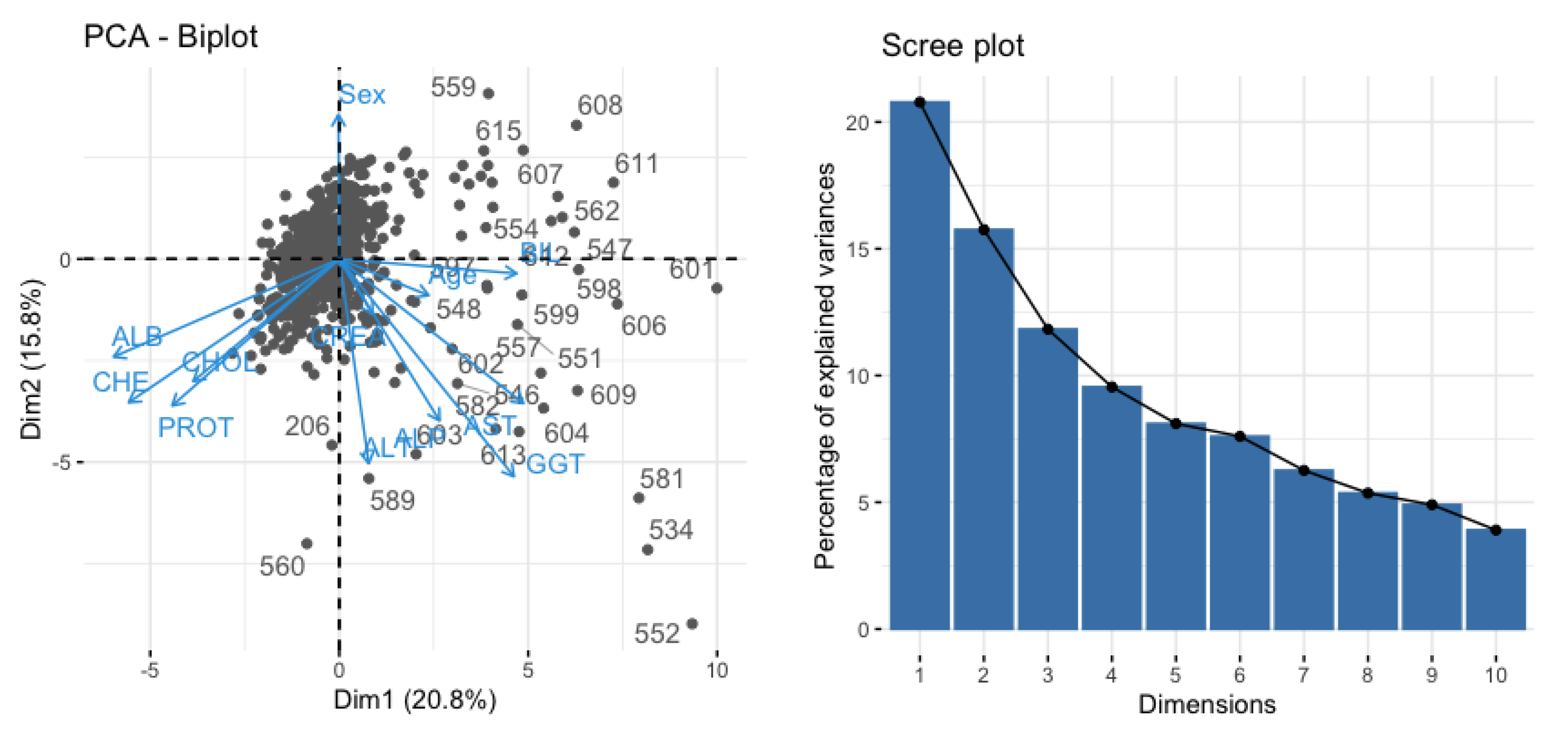
The PCA reduces the dimensionality by projecting each data point into the first few principal components to obtain lower-dimensional data and keep preserving maximum information. In Figure 7, a scree plot (right) is shown to determine the number of input variables. Figure 7 (left panel) shows the principal components with the variables AST, ALT, ALP, BIL, and GGT with almost 85% variability.

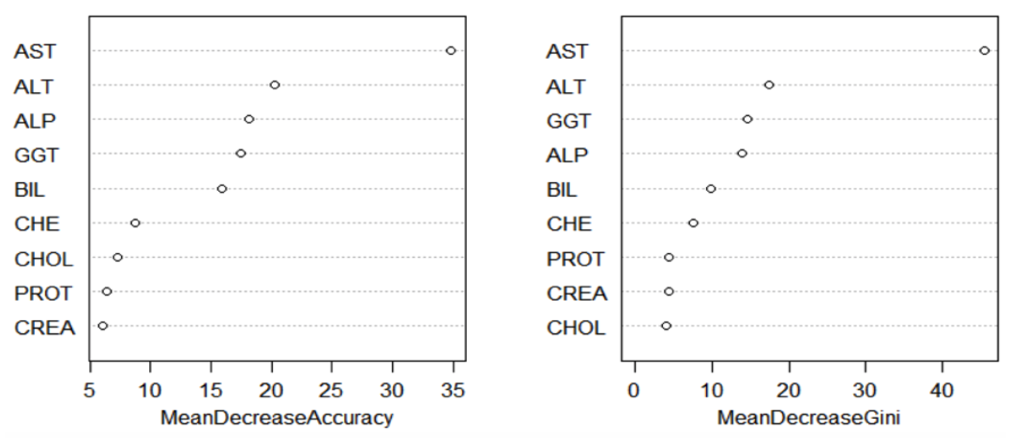
The variable importance ranking was obtained for RF, and it was measured using the mean decrease in accuracy and mean decrease in Gini as parameters. From Figure 8, AST, ALT, ALP, BIL, and GGT were the most important variables observed in the data set. After comparing with Figure 5 and the results from the PCA, AST, ALT, ALP, BIL, and GGT were used to train the classification models. To confirm the importance of the four variables for disease diagnosis, the following methods determined each variable association with the risk of liver disease development.

A logistic regression method was performed to calculate the odds ratios and 95% confidence intervals and to determine an association between risk factors and the occurrence of a liver disease. To reduce the effect of multicollinearity, a correlation analysis among independent variables was conducted, and those which had a variance inflation factor (VIF) greater than three were removed [34]. Considering liver disease with “no” as a reference group, AST (OR = 1.080, 95% CI: 1.050–1.111, p < 0.0001), ALT (OR = 0.981, 95% CI: 0.967–0.995, p = 0.010), ALP (OR = 0.954, 95% CI: 0.935–0.972, p < 0.0001), BIL (OR = 1.080, 95% CI: 1.032–1.130, p = 0.001), and GGT (OR = 1.023, 95% CI: 1.014–1.032, p < 0.0001) were found to be significant risk factors for liver disease. The logistic regression results validated the importance of AST, ALT, ALP, BIL, and GGT as risk factors for liver disease and indicated the success of the dimension reduction.

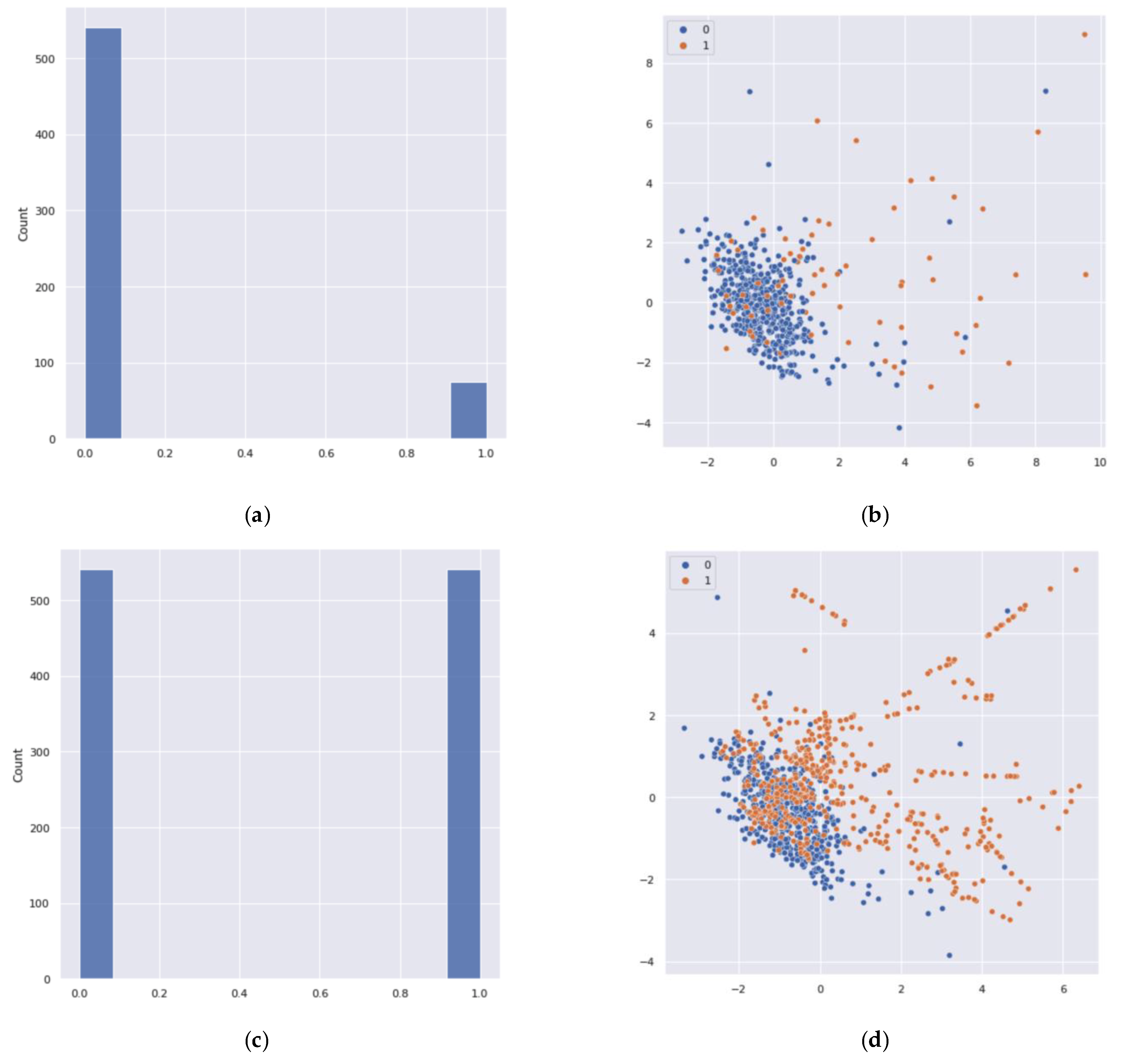
After analyzing the classification performance of the training set, a data imbalance problem was detected in the class labels. It caused the data overfitting problem in the binary classification technique. Thus, it resulted in an inaccurate performance measure of the classification. To solve this issue, an oversampling method was applied. To create a balanced data set for the minority class, the synthetic minority oversampling technique (SMOTE) [45] was applied. SMOTE is based on the nearest neighbor algorithm to generate new and synthetic data that can be used for training the model. Python, using functions from Pandas, Imbalanced-Learn, and the scikit learn libraries, was used to produce the synthetic data to overcome this problem (see Figure 9). After applying the SMOTE, 509 samples were added to the minority class.

Before applying binary classification ML methods on the testing data set, the models were trained, and before the training, the hyperparameter of each model was optimized. Hyperparameter tuning was exercised based on different combinations of parameters using a trial-and-error method to obtain the best model with less entropy. Hyperparameters were optimized for the neural network to determine the network’s structure as well as learning rate of the network. The sigmoid function was used in the output layer to obtain binary predictors. There were six neurons in the input layer to reduce the overfitting. Adaptive moment estimation (Adam) was used to obtain the model by minimizing the cost function, and in the fitting of the ANN model, the batch size was 32 and the epochs was 30. RF is a meta-estimator that fits several decision tree classifiers on various subsamples of the data set using averaging to improve the predicted accuracy and to control the overfitting. Thus, the number of trees in the forest was 10 using a trial-and-error basis. Gini criteria were used to obtain trees, which measured the quality of the optimal split from a root node. The SVM was trained with the radial basis function (RBF) kernel with two parameters (i.e., C and gamma), where the tuning parameter C was chosen as 10, and gamma was defined by how much influence a single training example had shown.

The results from the correlation matrix described each model’s ability to correctly classify the data. In

Table 2. Confusion matrix with class prediction using ANN, SVM, and RF.

Confusion Matrix	Actual Class			Actual Class			Actual Class
Predicted Class	ANN	0	1	SVM	0	1	RF	0	1
	0	100	5	0	101	4	0	104	1
	1	19	92	1	3	108	1	3	108

, three samples fall in the false positive group and one sample falls in the false negative group for RF classifier model. An interesting result was observed for RF: there were no FP samples in the testing data set. From the matrix, we can determine each model’s sensitivity, which evaluates the described model’s ability to predict true positives for each available category and the specificity which evaluates the model’s ability to predict true negatives for each available category. A summary of model evaluation is given below.

In

Table 3. Summary of the model evaluation.

Model	ANN	RF	SVM
Sensitivity	0.9523	0.9904	0.9619
Specificity	0.8288	0.9729	0.9729
Precision	0.9484	0.9908	0.9642
Accuracy	0.8889	0.9814	0.9675
${\mathit{F}}_{\mathbf{1}}$	0.8845	0.9817	0.9685

, RF shows the highest sensitivity value of 0.9904. SVM performed better than other methods in the context of running time. However, RF achieved the highest accuracy among the models. Among the three methods, ANN showed the poor performance. These results were also confirmed by the AUC–ROCs. Later five-fold cross-validation pair t-tests are presented to compare significant differences between the two binary classification techniques.

The AUC–ROC curves [46] of the classification validates the applied techniques for a good accuracy level. Moreover, 0–1 loss function supports the above results, where RF showed the lowest expected loss of 1.86%, which is very low. The diagnostic performance of the implemented tests or the accuracy of the tests for differentiating liver disease patients from normal healthy controlled individuals was evaluated using ROC analysis. This curve was used to compare the diagnostic performance of two diagnostic tests [47]. From Figure 10, all the machine learning methods performed well, because the value of the area under the ROCs were 0.98 for RF and exactly 0.97 for SVM. However, for the ANN, the area under the curve was approximately 0.89. The 95% confidence intervals for the ANN, SVM, and RF were 0.87 and 0.91, 0.96 and 0.98, and 0.96 and 0.99, respectively. The $p$-values for all of the ML methods were very small ($p<0.001$). Thus, it was concluded that the area under the ROC was significantly different from the value of 0.5. A significance level of α = 0.05 was assumed for rejecting the null hypothesis that both algorithms performed equally well on the data set and conducted the five-fold cross-validated t-test.

Since

Table 4. k-Fold cross-validation hypothesis test.

${\mathit{H}}_0: \mathbf{ANN} \mathbf{and} \mathbf{RF} \mathbf{Are} \mathbf{Equivalent}$	${\mathit{H}}_0: \mathbf{ANN} \mathbf{and} \mathbf{SVM} \mathbf{Are} \mathbf{Equivalent}$	${\mathit{H}}_0: \mathbf{SVM} \mathbf{and} \mathbf{RF} \mathbf{Are} \mathbf{Equivalent}$
t-Statistic: 1.285	t-Statistic: −1.221	t-Statistic: 0.945
p-Value: 0.231	p-Value: 0.253	p-Value: 0.369

presents $p>\alpha$, we could not reject the null hypothesis, and it was concluded that the performances of the two algorithms were not significantly different.

Furthermore, both minority and majority groups are important to classify between individuals with liver disease and without liver disease. First, the imbalanced data may deteriorate the performance of classification. Without using SMOTE when ML binary classification techniques were applied, their predictions mostly referred to the majority class and ignored the minority class. SVM performed slightly better than ANN and RF, where the minority class featured as noise in the data set, and it tried to ignore them when the models provided the outputs. It was predicted that only 15–16% of individuals in the minority class showed a highly biased nature to the majority class. However, after applying SMOTE, it was found that RF performed slightly better than SVM and sufficiently better than ANN (see Table 2). Therefore, there was evidence that the laboratory for liver disease diagnostic test does have a propensity to discern between patients with liver disease and non-liver disease. There are many examples of improving healthcare using machine learning [11,27,34,45,48]. Thus, this method can be used for improving medical diagnosis.

4. Conclusions

Chronic liver disease is detected by clinicians who are well trained in identifying significant observations and classifying them as normal or abnormal using background information and other context clues. ML algorithms can be trained to detect the possibility of liver disease in a similar way to assist healthcare workers. Using the correlation of each variable with the risk of liver disease to train the model, ML methods were able to identify which blood donors were healthy and which had liver disease with high accuracy. The PCA results showed five important factors for liver disease diagnosis: AST, ALT, GGT, BIL, and ALP. In a real situation, a clinician can strongly suspect liver disease using only these five variables, as they are very descriptive for liver function. The ratio of ALT and AST can denote the cause of a liver injury. GGT and ALP increase in circulation with the severity of a liver injury. Additionally, the injury proximity to the bile duct can be determined by the concentration of ALP. Validation of these four variables for diagnosis was further seen using the Gini index. This study showed several machine learning approaches with PCA, which outperformed the classification. Among three ML classification methods, SVM and RF performed better than ANN. Although, the accuracy levels for all three methods performed well based on the testing data set. SMOTE produced very effective results in classification performance by oversampling the minority group.

In the future, the local interpretable model-agnostic explanation (LIME) method will be used to understand the model’s interpretability. Instead of binary classification, one may use multinomial classification by separating the types of liver disease. In this way, each model’s performance can be compared. The described ML methods can assist health sectors to achieve a better diagnosis providing effective results in identifying groups or levels within medical data to facilitate healthcare workers. Moreover, ML methods are data driven, and they directly use diagnostic variables from patients’ medical tests. Thus, it is a more reliable process. The applied ML methods in this article can save time, costs, and potentially lives for the betterment of disease diagnosis.

The machine learning algorithms presented in this study can support medical experts but are not the alternative when making decisions from ML classifiers for diagnostic pathways. These methods can reduce many of the limitations that occur in healthcare associated with inaccuracy in diagnoses, missing data, cost, and time. Application of the ML methods can help reduce the total burden of liver disease on public health worldwide by improving recognition of risk factors and diagnostic variables. More importantly, for chronic liver disease, detecting liver disease at earlier stages or in hidden cases by ML could decrease liver-related mortality, transplants, and/or hospitalizations. Early detection improves prognosis, since treatment can be given before progression of the disease to later stages. Invasive tests, such as biopsy, would occur less in this case as well. Although this study focused on hepatitis and chronic liver disease variables for ML training, it can be hypothesized that the methods can be used to distinguish other types of liver disease from healthy individuals. Applying all of the mentioned methods to other areas of medicine could open the doors for AI/ML-facilitated diagnosis.