Article

Initiating Event Frequencies for Internal Flooding and High-Energy Line Break PRAs

by
Karl N. Fleming
1,*,
Bengt O. Y. Lydell
2,
Mary Presley
3,
Ali Mosleh
4 and
Wadie Chalgham
4
1
KNF Consulting Services LLC, Spokane, WA 99205, USA
2
Sigma Phase Inc., Vero Beach, FL 32967, USA
3
Electric Power Research Institute, Charlotte, NC 28262, USA
4
B. John Garrick Institute for the Risk Sciences, Henry Samueli School of Engineering and Applied Science, University of California at Los Angeles, Los Angeles, CA 90095, USA
*
Author to whom correspondence should be addressed.
J. Nucl. Eng. 2025, 6(3), 37; https://doi.org/10.3390/jne6030037
Submission received: 14 May 2025 / Revised: 12 June 2025 / Accepted: 22 August 2025 / Published: 16 September 2025
(This article belongs to the Special Issue Probabilistic Safety Assessment and Management of Nuclear Facilities)

Abstract

Utilities that operate nuclear power plants are increasingly using probabilistic risk assessments (PRAs) to make day-to-day decisions on design, operations, and maintenance and to support risk-informed applications. These applications require high-quality and complete PRAs to ensure that the decisions and proposed changes are technically well-founded. Such PRAs include the modeling and quantification of PRA models for accident sequences initiated by internal floods and high-energy line breaks. To support PRA updates and upgrades for such sequences, the Electric Power Research Institute (EPRI) has sponsored ongoing research to develop and refine guidance and generic data that can be used to estimate initiating event frequencies for internal flood- and high-energy line break-induced accident sequences. In 2023, EPRI published the fifth revision of a generic database for these initiating event frequencies. This revision produced advancements in the methodology for passive component reliability, including the quantification of aging effects on pipe rupture frequencies and the capability to adjust these frequencies to account for enhancements to integrity management strategies associated with leak inspections and non-destructive examinations. The purpose of this paper is to present these enhancements and illustrate their application with selected examples.

1. Introduction

The purpose of this paper is to summarize recent developments in the modeling and quantification of accident sequences initiated by internal floods and high-energy line breaks that are documented in a recent report published by EPRI. This EPRI report is available to the public at http://epri.com and is subject to a license fee [1]. This report is the latest in a series of reports that document a study to develop estimates of piping system flood frequencies for use in probabilistic risk assessments (PRAs) consisting of accident sequences induced by internal flooding (IF) and high-energy line breaks (HELBs). Previous versions of this report [2], and the companion documents [3,4], have covered most piping systems outside the containment in pressurized water reactors (PWRs) and boiling water reactors (BWRs) that can produce flooding or high-energy line breaks (HELBs) based on an analysis of operating experience in U.S. and selected foreign light-water reactor (LWR) plants. This report updates the flood frequencies to account for service experience through the end of 2020. Guidance for the performance of internal flooding and HELB PRAs making use of the flood frequency data in this report series was published in Reference [5]. The EPRI-sponsored work in this area is developed to meet the technical requirements of the ASME/ANS PRA Standard for internal flooding PRAs [6]

2. Technical Approach

2.1. Overview

The model used to estimate internal flood-induced initiating event frequencies in Reference [1] is based on that used in previous revisions to this report [2,3] and is the fifth revision to a series of reports that EPRI has published to support internal flooding PRAs (IFPRAs) in the nuclear industry. Each revision has expanded the scope of covered piping systems and has tracked the trends in piping system performance due to pipe degradation.
One of the motivations in issuing these revisions is to address user feedback and requests for more guidance in the performance of IFPRAs. Because failure rates have been trending upwards due to piping system degradation, it has been necessary to provide updates to keep the predictions current. In addition, plants have been backfitting corrosion-resistant materials to replace carbon steel piping that has added additional scope of piping systems.
In this latest revision, significant enhancements were made to enhance the capabilities of the pipe failure models to provide flood frequencies that are in alignment with those observed in the service data. The basic pipe failure model used in all the revisions was originally developed to support risk-informed in-service inspection (RI-ISI) programs [7,8,9]. For that application, it was subjected to independent reviews by the University of Maryland [10,11], Los Alamos National Laboratory [12], and the U.S. Nuclear Regulatory Commission [13]. This method is similar to that used in NRC studies on LOCA initiating event frequencies [14,15]. The method addresses and quantifies the impacts of many sources of uncertainty in the estimation of piping system flood frequencies as described more fully in this paper. Improvements to the methodology and data analysis that were made in Reference [1] address the impact of aging due to pipe degradation and include guidance on how integrity management strategies can be employed to reduce the frequency of pipe rupture.
A key element of the methodology is the approach to treating factors that influence pipe system reliability. Such factors include the pipe materials, pipe design codes, pipe degradation mechanisms, frequency and effectiveness of pipe inspections for cracks, wall thinning and leaks, operating conditions including temperature, pressure and fluid properties, pipe size, and other factors. These factors are addressed by defining a comprehensive set of homogeneous pipe failure cases within which the reliability characteristics are preserved. Piping systems are broken down into categories based on operating conditions, design codes, pipe materials, applicable failure mechanisms, and pipe sizes, and separate flood frequency metrics are developed for each. Consistent with current industry practice in internal flooding and high-energy line break PRAs, the scope of piping systems covers all piping systems in PWR and BWR plants outside the containments, including safety-related and non-safety-related piping systems.

2.2. Technical Enhancements from Previous Revision

The overall technical approach—described in detail in Section 2.3—generally follows the technical approach from previous revisions of this report, but with some significant enhancements. The term “pipe failure” in this model is defined as any pipe failure mode that requires repair and replacement and includes cracks and wall thinning that exceed repair and replacement criteria in the design codes, leaks, and ruptures. All such defined pipe failures are regarded as precursors to a more serious failure mode. The frequencies of leaks and ruptures are estimated as the product of the failure rate and a conditional probability of failure which is dependent on break size. All refinements to the methodology have been independently reviewed by a third party, as documented in Appendix G of Reference [1]. The enhancements include an expanded coverage of piping systems, quantification of the effects of aging, improvements to estimating the conditional probability of pipe rupture given failure, impact of integrity management strategies, a wider set of flood frequency metrics, and improved guidance for use of the data in internal flooding PRA.
Below is a summary of enhancements to the technical approach achieved in Reference [1] in comparison to those in a previous revision [2].

2.2.1. Expanded Coverage of Piping Cases

The Revision 5 Report [1] includes flood-induced initiating event frequencies for an expanded set of piping types and sizes in comparison with the previous [2]. New service water system cases were added to address corrosion-resistant piping that has been backfitted into plants to address degradation in the original carbon steel piping. In a similar vein, additional cases were added to address plants who have incorporated stainless steel piping for high-energy piping systems to mitigate the effects of flow-accelerated corrosion. In addition, for all the systems addressed in previous report revisions, new cases were added to address different pipe sizes that were previously addressed using a cumbersome interpolation procedure. While most of the flood frequency cases are associated with piping, some selected components that have been found to be risk-significant are also included.
Table 1 provides a comparison of pipe cases in Revision 5 [1] versus those found in a previous revision [2] of this report (items new to Revision 5 are in bold italics; items that were removed or merged from the previous revision are in strikeout text).
The distinct failure rate cases reflected in Table 1 were defined to isolate the most significant factors that were found to impact piping system reliability, with the focus on the piping systems found to be the most important in IFPRA, which are the service water system piping and the fire protection system piping. Both of these systems have large or open-ended sources of flood water, are found in flood areas with many SSCs modeled in the IFPRA, and are responsible for the major part of flood-induced accident sequences to model in an IFPRA. For the service water system alone, Table 1 includes 198 different cases covering combinations of reactor type, water type, pipe size, pipe materials, and design codes. The definition of these cases is based on a detailed review of the pipe failure events in the PIPExp database that was used for the counts of different pipe failure modes that go into the flood frequency estimates. PIPExp is discussed further in Section 2.2.7.

2.2.2. Incorporation of Aging Effects

Previously, flood frequencies have been estimated based on the average performance of the piping systems over their experienced service life. To account for observed increasing trends in average failure rates in successive updates, the pipe failure model has been enhanced to incorporate the effects of aging due to the accumulated effects of degradation. Revision 5 of the EPRI report uses an updated pipe failure model that includes an adjustment to the average flood frequencies to account for the age of the pipe. Aging factors are based on trends that are observed in the average failure rates over five-year intervals in the life of the pipes. There was sufficient data to apply this approach to service water and fire protection water systems that cover most of the risk-significant piping segments identified in internal flooding PRAs. There was insufficient data to support the development of other piping systems in the scope of the evaluation. The methodology and selected results for the treatment of aging is discussed in Section 3 of this paper.

2.2.3. Enhanced Conditional Probability of Rupture Model

The pipe failure model described in Section 2.3 of this paper expresses pipe rupture frequencies as the product of a failure rate and a conditional probability of pipe rupture. The model for estimating the conditional rupture probability (CRP) given pipe failure that has been used in previous revisions to this report has been enhanced to provide more realistic estimates of flood frequencies. Instead of using one CRP model for all pipe sizes, in this revision, different CRP models are used for different pipe sizes. A new method was introduced to address modeling uncertainty more systematically. A calibration step was added to ensure that predicted flood frequencies are in alignment with industry data. More details on the CRP model enhancements are provided in Section 4 of this paper.

2.2.4. Adjusting Flood Frequencies for Enhanced Integrity Management

Previous versions of the report included integrity management factors to adjust the flood frequencies to account for changes in the surveillance programs for leak inspections and non-destructive examinations to improve performance. However, user feedback indicated these factors were difficult to credit in a practical manner. To address this feedback, Revision 5 has introduced a limited set of pre-defined integrity management strategies linked to specific procedures, including one for standard industry practice and four strategies that can credit various levels of leak inspection and non-destructive examination (NDE) testing that is expected to be more effective than standard industry practice. These factors should only be applied to the most risk-significant pipe segments that receive extra inspection rather than to the entire piping system. Adjustment factors have been developed for each of these integrity management strategies using the Markov model that was originally developed for the risk-informed in-service inspection programs [9]. The base flood frequencies developed in the Revision 5 report reflect the standard industry practice for tests and inspections to check for piping system leaks and for application of non-destructive examinations (NDEs) to identify cracks and flaws. The adjustment factor for standard practice is 1.0. Adjustment factors less than one may be applied for each of the enhanced strategies that involve enhanced surveillance for leaks, enhanced NDE, or both. More details on this approach are provided in Section 5 of this paper.

2.2.5. Expanded Set of Flood Frequency Metrics

For each analysis case, an improved method for presenting flood frequency results has been employed that includes 3 metrics of flood frequencies to support different levels of refinement:
  • Cumulative break frequency of different break sizes and flood rates
  • Flood frequencies for basic flood modes (spray, flood, and major flood)
  • Flood frequencies for more refined flood rate intervals
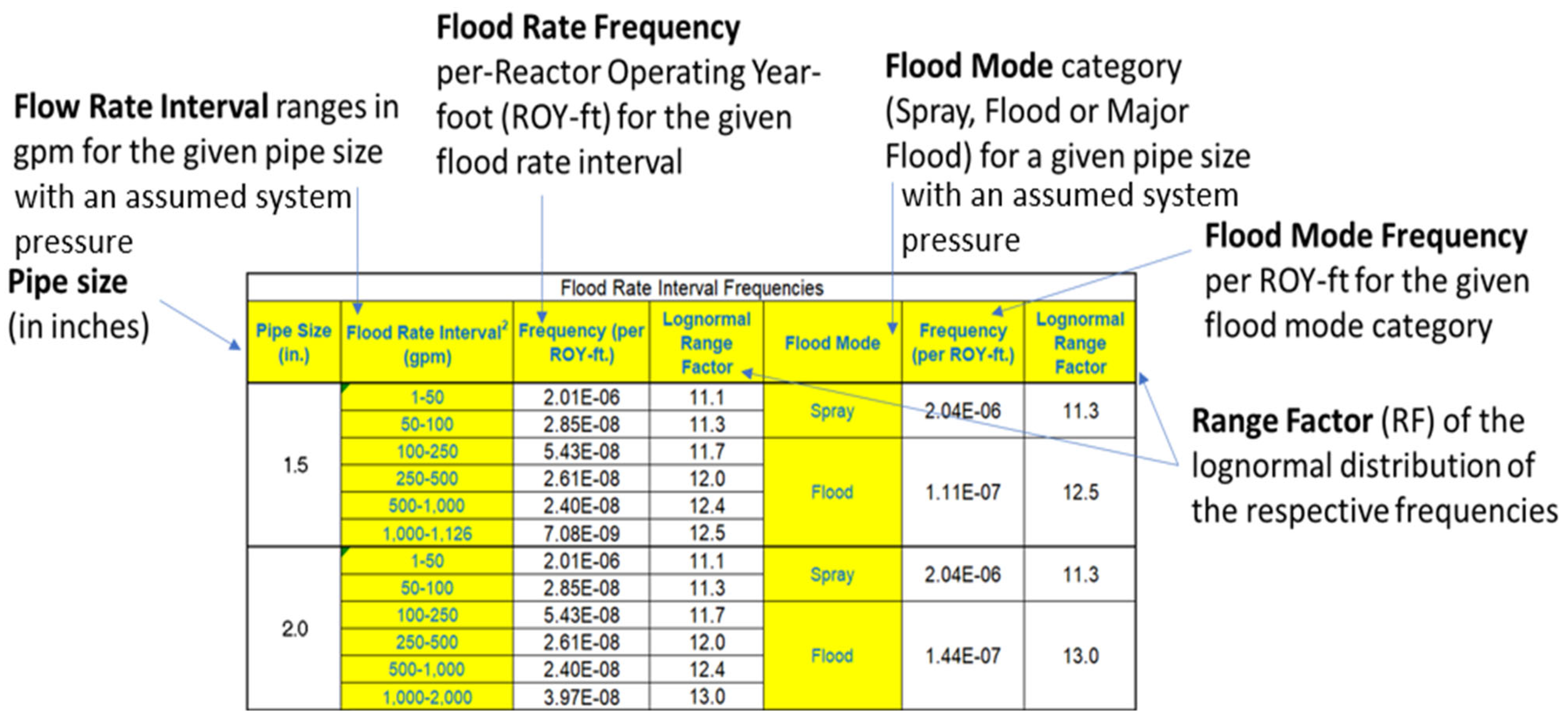
Each flood frequency metric is presented using mean values and range factors of lognormal distributions that have been fitted to the results of the flood frequency uncertainty analysis. Rather than presenting the flood frequencies in the form of report tables as in previous revisions, for ease of use, the flood frequencies and adjustment factors developed in this report are provided in the form of Microsoft Excel spreadsheets and input files for use in the FRANX software, Version 11 [16]. This software provides the ability for the user to apply the Revision 5 flood frequency data to develop flood-induced initiating event frequency models that interface with EPRI-developed software for PRA modeling of flood-induced accident sequences. With this software, the user may easily modify the flood frequency data to eliminate the need for the user to make calculations to adjust for differences in defining flood rate ranges, system operating pressures, unusual pipe sizes, etc. Details on the flood frequency metrics are presented in Section 6.

2.2.6. Roadmap

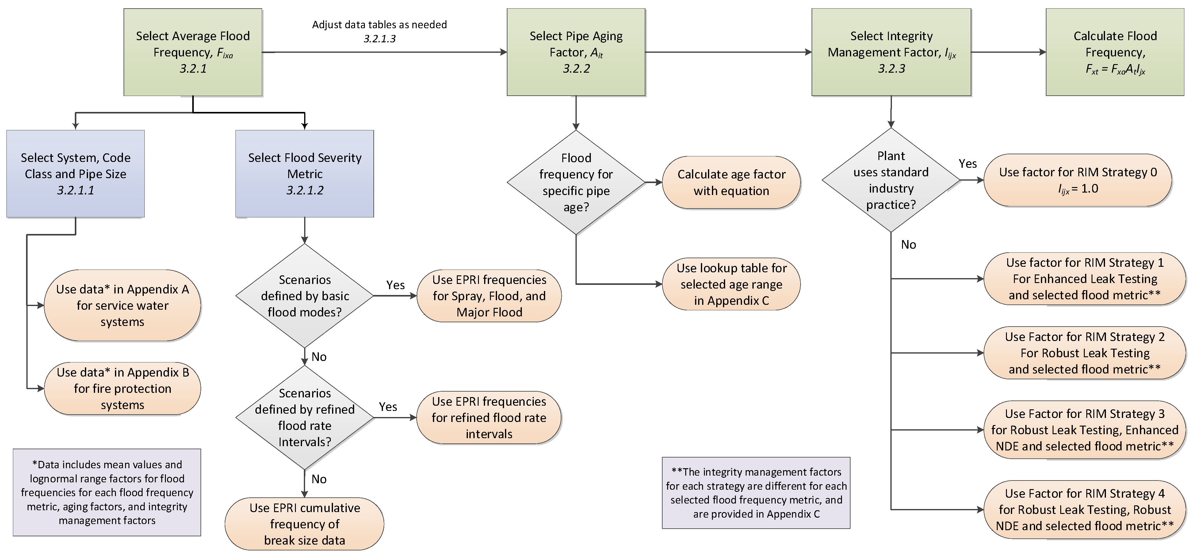
The Revision 5 report includes a new user’s guide for application of the flood frequency data provided in this report, including how to select the appropriate flood frequency analysis case for the user’s application, how to adjust data for plant-specific pipe sizes and system pressures, as well as how to apply aging factors and integrity management factors. An example application of the roadmap is provided in Section 7.

2.2.7. Service Experience Data

To implement the technical approach for estimating flood frequencies, a comprehensive pipe reliability database was required. The source of pipe failure and exposure data used to quantify the failure rates used in these models is known as PIPExp, as described in Appendix H of Reference [1]. The PIPExp database is a continuously updated and maintained database that was established in 1994. The database covers the period 1960 to date and includes pipe failures in BWRs, PWRs, RBMKs, VVERs, heavy water reactors, gas-cooled reactors, and liquid metal-cooled reactors. Although PIPExp is a proprietary database, all the information that is included comes from public domain sources. The database content consists of information extracted from Licensee Event Reports (or equivalent event reports), Condition Reports, Action Requests, in-service inspection (ISI) reports, ASME XI code repair relief requests, operability determinations, metallographic evaluation reports, work orders, laboratory reports, private communications, and collaborative work. This database has been relied upon as a source of data on pipe failure events to support generic estimates of LOCA initiating event frequencies [14,15] and numerous other applications. The results of applying it are presented in the subsequent sections of this report. The Revision 5 report looks at service data from January 1 1970 through 31 December 2020.
The service experience data is organized by system, pipe size, failure mode (non-through wall defect, pinhole leak, leak, and major structural failure), pipe system age at the time of failure, and damage/degradation mechanism. Failure modes include the following:
  • “Non-through wall defect” or “Wall Thinning”—a Code-rejectable defect that requires repair or replacement according to the prevailing codes and standards.
  • “Pinhole leak”— characterized by both defect size and leak rate; the leak rate is equal to a “perceptible” leakage that is less than, or much less than 1 gpm.
  • “Leak”—through-wall defects that are normally expected to have leak rates ≥ 1 gpm.
  • “Major structural failure” (MSF)—a complete loss of structural integrity and consequential significant through-wall flow rate.
Note: All through-wall failures are classified by equivalent break size for the leak. The equivalent break size (EBS) is defined as the diameter of a circular hole that produces a specified flood flow rate calculated using a choke flow equation. This form of the data is used to inform the calculation of conditional probability of break sizes via the CRP model.
Metallic piping failure is due to single or multiple damage mechanisms, or combinations of damage and degradation mechanisms. Piping failure propensity is a function of operating environment, pipe stresses, and fracture toughness of the material. Damage mechanisms are event based. That is, some pre-condition must exist for a failure to occur. Examples of damage mechanisms include metal fatigue through low-cycle and high-cycle pressure loading, and thermal fatigue.
By contrast, degradation mechanisms (or environmental degradation) are time-dependent events. The incubation time of degradation mechanisms depends on a critical combination of metallurgical variables (alloying elements), environmental variables (e.g., water chemistry, local flow conditions, temperature), and stress variables (e.g., service stress, fit-up stress, residual stress, strain stress).
The failure propensity varies extensively across the range of piping systems evaluated in this study. It depends on the damage and degradation susceptibility. Certain degradation mechanisms result in through-wall defects if left unmitigated. Some failures can propagate rapidly if a system transient results in a sudden hydraulic or mechanical load. Alternatively, failures may show up as pin-hole leaks that can be repaired before the consequences become more significant. Under certain conditions (e.g., thick-wall, high-strength piping material), degradation may not propagate beyond “part through-wall.” Because of this variability, flooding from failure of the pipe is dealt with statistically through the pipe rupture model, discussed in the next section.

2.3. Pipe Rupture Model

The pipe rupture frequency distribution presently cannot be calculated directly from the service data for all pipe sizes because of insufficient data, particularly for the rarer pipe rupture events. To derive the pipe rupture frequency, then, a model is used for relating failure rates and rupture frequencies, which is widely used in piping reliability assessment [10].
This model, expressed in Equation (1) and described further below, calculates the pipe rupture frequency ρ i x t for a given pipe category i as the product of the pipe failure rate λ i , the conditional probability of a pipe rupture given that a failure has already occurred P R x F using the conditional rupture probability (CRP) model, the aging factor A i t and the integrity management factor I i x .
ρ i x t = λ i P i R x F A i t I i x
where
  • ρ i x t = total rupture frequency for pipe category i defined by analysis case and pipe size for rupture mode x at pipe age t.
  • λ i = failure rate of pipe category i.
  • P i R x F = conditional rupture probability (CRP) of rupture mode (i.e., severity of rupture) x given failure of pipe component i. See Section 4 for development of the CRP model.
  • A i t = age factor for component i at pipe age t to account for in-service degradation due to aging of the component. See Section 3 for the derivation of aging factors.
  • I i x = integrity management factor for component i and rupture mode x; this factor adjusts the rupture frequency to account for variable integrity management strategies such as leak detection, volumetric NDE, and in-service testing that might be different from the components in the service data. See Section 5 for the application of the Markov Model for derivation of these integrity management factors.
Figure 1 provides a flow chart of how the pipe failure rate is developed from the data and combined with the conditional rupture probability P R x F to create the flood frequency ρ i x t with key steps for the treatment of uncertainty.
To calculate the pipe failure rate λ i , a broad generic prior distribution is used, generally based on system-specific pipe failure rates developed for the EPRI RISI program [8]. To address uncertainty in the prior distribution, the Constrained Non-Informative Distribution (CNID) method is used, in which the mean value of a gamma distribution is anchored to the mean estimate from [11]. The pipe failure rate is expressed in units of failures per reactor operating year-foot (ROY-ft). “When applied in a PRA, the flood frequencies in ROY-ft should be adjusted by the plant availability to produce flood frequencies per calendar year, as called for in the PRA Standard [6]. The generic prior is then updated using a Bayesian approach with data for the numerator (number of failures) and denominator (component-years).
For the IFPRA application, the definition of a component for most cases is “linear-foot of piping system”. In a typical IFPRA, there are several kilometers of piping that must be analyzed, and these are divided up into flood areas that typically have many piping system components including straight runs of pipe, welds, pipe and valve bodies, heat exchangers, flanges, elbows, tees, etc. For practical application of the EPRI data, the failure rates for most cases are developed in terms of failures per linear foot of piping system that captures all the components in a piping system. It is not practical to develop separate failure rates for each component as the vast majority of pipe failures occur in the pipes and weld connections to other components. However, the same assumption is made in the development and application of the data. There are special cases where a flood area only contains a valve or pump and very short runs of piping, in which case frequencies are developed on a per component basis. Another special case is rubber expansion joints, and in this case, failure rates and rupture frequencies are developed in terms of events per component-year. For risk-informed inservice inspection applications that focus on changing weld inspection locations, failure rates and rupture frequencies are developed on a per weld-year basis. Examples of this application are provided in Reference [7].
For the pipe failure frequency, the failure count (numerator) is taken from the service experience database. Specifically, the count includes all failures from the U.S. events in that database for a given pipe category which is defined in terms of the system, pipe design and material, and pipe size. For this count, a “failure” is defined as any event requiring repair or replacement of the pipe, including wall thinning, cracks, leaks, and ruptures of various sizes up to and including complete severance of the pipe. The failure rate is estimated based on the average performance of the component over the industry service life from which the data is collected.
The reactor operating year-feet (denominator) is a distribution that combines reactor operating year (ROY) data with pipe lengths. Estimates for the ROY in the service data are based on sources of generic data identified in Reference [1] on the reactor critical hours in each calendar year for each plant. Estimates of pipe lengths per plant are developed by reviewing isometric piping diagrams for a representative sample of plants. The uncertainty treatment methodology described in Section 2.5 addresses uncertainty in extrapolating these measurements to the plant population.
An estimate of the total length of pipe for each pipe case is developed in the pipe failure database based on a review of piping system isometric diagrams for a sample of plants. To address the uncertainty and variability in pipe lengths across the industry, an uncertainty treatment that was originally developed for the EPRI RISI program [10] was applied as follows: A probability of 0.5 is applied to the pipe length estimate obtained from the isometric review for the sample of plants. A probability of 0.25 is applied to the assumption that the pipe length is 50% larger and 50% smaller than the best estimate. These probability assignments are made based on the expert opinion of the authors, taking into account the sample size of the number of plants, approximately a dozen, in the industry for which measurements of pipe lengths were made from isometric piping diagrams. This approach was considered more realistic that simply making an optimistic assumption that the sample measurements were representative of the entire industry. The upper and lower bounds of this pipe length model provide a reasonable bound on the estimate. It was impractical to measure the pipe lengths for the entire industry of more than 100 reactor plants.
Then, three Bayes’ updates are performed by updating the generic prior distribution with the failure counts and three different exposure terms obtained by multiplying the reactor operating years times the pipe length estimates. Using a Monte Carlo sampling procedure, the results from these three Bayes’ updates are combined using the mixture distribution method, producing the uncertainty distribution for the failure rate for the given pipe case.
This pipe failure model and the supporting Markov model, minus the aging factor, have been used in many applications and has been extensively peer reviewed as discussed more fully in Section 6.

2.4. Treatment of Leak-Before-Break

This model assumes that every failure event is a precursor to a rupture, i.e., each time a failure is repeated, it challenges the integrity of the pipe and, in some cases, leads to a pipe rupture. The degradation mechanisms responsible for all pipe failures are documented in the EPRI reports and they are generally the same for non-through wall defects, small leaks, and ruptures. This assumption is common among passive component reliability models used in PRAs [14,15]. The end state of a given degradation mechanism as to how far it progresses until discovery is dependent on many factors including the geometry of cracks, pipe stresses, and method of discovery. A common question from users is ‘how does this methodology credit Leak-Before-Break’?
Leak-Before-Break (LBB) is a set of evaluation (analytic) criteria to justify the exclusion of dynamic effects of pipe ruptures (e.g., to justify the removal of pipe restraints and pipe whip protections). It is a deterministic evaluation that demonstrates sufficient margins against failure, including verified design and fabrication, good fracture toughness properties of the pipe material, and an adequate integrity management program to find flaws and leaks and repair and replace the affected components thereby preventing pipe ruptures. Material selection (and associated facture toughness) for piping is driven by codes and standards. LBB analyses serve to confirm adequate fracture toughness
The concept of LBB is accounted for in this evaluation of flood frequencies as follows:
  • The failure rate provides an estimate of the frequency of precursors to leaks and ruptures.
  • Conditional rupture probability (CRP)—provides an estimate of the probability that a failure produces a leak or rupture. An effective application of LBB is reflected in a low CRP for major pipe ruptures. The service data includes the benefits of LBB in that it inherently includes all expected opportunities to spot the leak that would occur at a typical plant (including things like normal operator rounds, security rounds, quarterly leak inspections, NDE inspections).
  • Integrity Management Factors (Markov Model)—to account for improvements beyond typical industry practice for leak testing and non-destructive examinations, integrity management factors are applied on an as-needed basis (see Section 5).

2.5. Treatment of Uncertainty

In the development of Bayesian uncertainty distributions for these parameters, prior distributions are developed for the parameters λ i and P R x F . As in standard Bayesian updating, these distributions are updated using evidence from the failure and exposure data. The exposure terms expressed in terms of reactor operating year and feet of pipe that produced the failures are uncertain because the estimates of pipe length per plant are based on a small subset of plants and must be extrapolated to represent the average across the entire industry represented in the data set for the failure counts in the numerator of this equation. The reactor years of service experience has a relatively small amount of uncertainty; therefore, this uncertainty is judged to be dominated by the uncertainty in the estimated pipe lengths per reactor. In this process, the uncertainty is treated by adopting three hypotheses about the values of the pipe length portion of the exposure terms, as described. The CRP treatment also incorporates elements of uncertainty including modeling uncertainty adjustments.
A tabulation of the steps in developing the flooding frequencies and how uncertainty is addressed in each step is provided in Table 2. The results of these steps are the mean and log normal range factor (RF) output provided in the Excel tables and FRANX tables for use in the IFPRA.
The Bayes’ models in the above table explicitly account for uncertainty in the sparsity of data. For the failure estimates in Steps 1 though 5 in Table 2, for each failure rate case, there are 3 Bayes updates of a Gamma prior distribution, one for each of the 3 different pipe length estimates. These make use of the conjugate properties of the Gamma distribution. The resulting posterior distributions are then combined producing a mixture distribution which is no longer a Gamma distribution. The mixture distributions are developed via Monte Carlo sampling. While there is generally a large population of failure events there are much fewer events involving large ruptures. The prior distributions for the CRP model undergo Bayes’ updating to incorporate the evidence on pipe failure modes from the service data. As noted above for Step 9, the updated beta distributions obtained in Step 7 and revised in Step 8 were converted to lognormal distributions to account for the uncertainty associated with the model assumption that pipe failures are precursors to ruptures and for applying the CRP model beyond the range of the supporting industry leak data. This increases the range of the CRP model uncertainty to account for this source of modeling uncertainty. In addition, the resultant beta distributions had very narrow uncertainty bands, and engineering judgement was applied to account for the model uncertainty. Although many pipe failures are available to inform the estimation of the pipe failure rates, for reliable systems such as Class 3 service water systems, there are much fewer pipe ruptures to consider in the Bayes’ updating in estimating the conditional rupture probabilities. To address the uncertainty associated with extrapolating a limited number of pipe ruptures, this additional step is performed to avoid understating the uncertainty reflected in the Bayes’ update. Otherwise, the calculated distributions would not address modeling uncertainty.
The lognormal distributions in the CRP model were assigned by conserving the means of the updated Beta Distributions and then assigning an error factor that increases with decreasing frequency. This step is specifically carried out to incorporate the modeling uncertainty reflected in the model in Equation (1), which assumes that all pip failures are considered to the precursors to pipe ruptures. The lognormal distribution range factors were set based on the following engineering judgments informed by the author’s experience in piping system reliability:
  • A RF of 2 was assigned to a P i R x F value of 1 × 10⁻²;
  • A RF of 30 was assigned to a P i R x F value of 3 × 10⁻⁵;
  • For specific P i R x F values other than the above, a RF was calculated based on log-log linear interpolation/extrapolation between these points.
The final frequency of pipe breaks as a function of break size are computed using Monte Carlo sampling. The frequencies of different break size are converted to flood flow rates using hydraulic equations for choke flow and a reference set of system pressures. The Roadmap in Section 3 of the Report provides guidance for modifying the flood flow rates for different pipe sizes and system pressures. The above steps are presented to document the process used to develop the flood frequencies in this report.

3. Conditional Rupture Probability Model

The conditional rupture probability, P i R x F is expressed as a fraction of failures of that given pipe component that develops into a pipe break for each pipe break size up to and including complete offset rupture of the pipe (double ended guillotine break, DEGB). The calculation begins with a generic prior distribution for each pipe case and is updated with the service data. The following four steps describe the generic development process for CRP models, as labeled 1–4 in Table 2.
  • Develop a prior distribution: A Bayes’ prior distribution is developed that incorporates insights from generic piping service experience and results of previous expert elicitations in the estimation of piping system reliability; sources for specific systems are documented in the report. This yields a table of CRP values vs. break sizes for each analyzed pipe size category. This is fitted to a CNID using the Beta Distribution by using the estimates as mean values and estimating the Beta Distribution parameters using the CNID method [17].
  • Bayesian update (Stage 1): A Bayesian update of the prior distribution is performed using evidence from service experience on frequency of leaks of different sizes for systems similar to those being analyzed. This yields a new Beta Distribution and reflects the combined evidence expressed in the prior and the industry service data.
For failure rate calculations, an event is classified and counted based on information contained in original source documentation. Part of this step includes reviewing and “cleaning up” the data used in the failure rates to establish a “best estimate” EBS for use in the CRP; this can include removing data where there is insufficient data to classify by size of leak, obtaining more information about specific events (work orders, inspection details, etc.) if available, augmenting the data with non-U.S. experience where the data supports it, and reclassifying or refining the classification of each failure.
3.
Bayesian update (Stage 2): A second stage Bayes’ update is applied to calibrate the CRP model to synchronize the predictions made by the pipe failure model with observed industry data on the frequency of leaks of different magnitudes. This step was added by observing that predictions made by the EPRI pipe failure model used in previous revisions to the failure report were somewhat over-estimating the frequency of leaks of different sizes observed in the industry service data.
The pipe failure model produces estimates of the flood frequencies per linear foot of piping system, per reactor year of operation (ROY). If we multiply the flood frequencies (per ROY-ft) from the previous step by the pipe exposure (ROY-ft) used to develop the estimates, a prediction is made of the number of events expected at each flood level. When this calculation is done, which is referred to as the “Bottom-up” prediction (predicted value), these predictions may be compared to the observed industry data which gives a “Top-down” perspective (actual value). In previous revisions, it was observed that the “Bottom-up” prediction can yield estimates that differ significantly from the observed service data. In this step, we modify the CRP values so that the “Bottom-up” prediction is in line with the observed leak data when large discrepancies are identified. This step is used as a way to calibrate the CRP model and may be viewed as a second step of Bayes’ updating of the original CRP prior which incorporates the new evidence from the Bottom-up vs. Top-down comparison.
4.
Apply Modeling Uncertainty: Adjustments are made to the uncertainty distribution of the CRP model to account for modeling uncertainty, as described in Section 2.5. This includes the basic assumption in the pipe failure model that pipe failures can be regarded as precursors to pipe ruptures of various sizes. This is done by converting the means of the Beta distribution from the Bayesian update of the CRP priors to means of a lognormal distribution in which the lognormal range factor (RF) expresses a larger degree of uncertainty than is reflected in the Bayes’ updated Beta Distribution. Lognormal range factors were assigned using systematic rules, as described in Section 2.5.
The failure rate distributions and CRP distributions for different pipe sizes are combined using a Monte Carlo simulation procedure to produce results in the form of cumulative frequencies for each break size and pipe size. For the systems with subcooled water (excluding the high-energy systems), reference system pressures from Reference [5] are used to convert the cumulative break frequency vs. break size to a cumulative flood frequency vs. flood rate in gal/min.

4. Evaluation of Aging Factors

4.1. Trends in Piping System Failure Rates

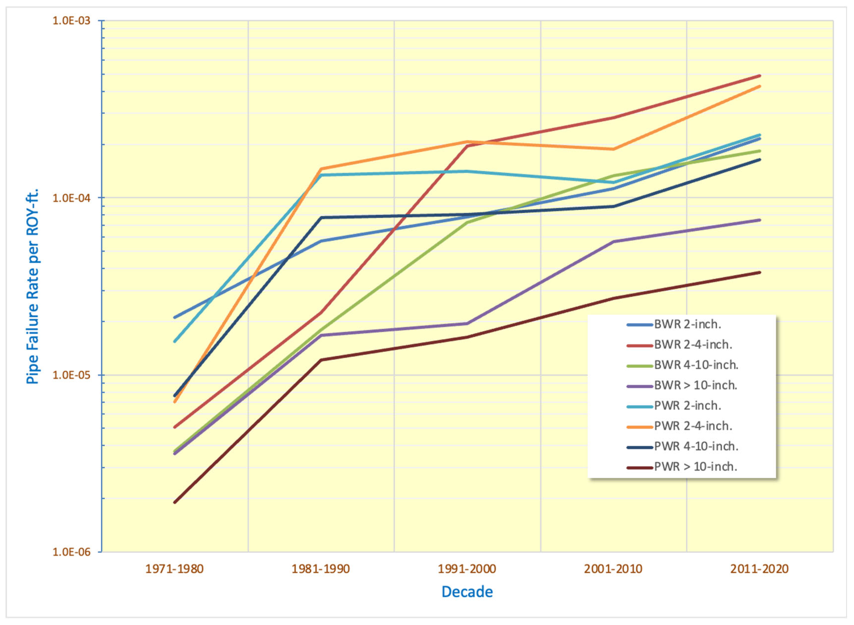
Since the initial publication of the EPRI flood frequency report series in 2006, the pipe failure rate estimation process for IFPRA and HELB analysis applications has undergone several revisions to reflect new operating experience data, an expanded scope of piping system coverage, and enhancements to the pipe failure model. In the 5th revision of the report, the pipe failure rate estimation process includes a step to account for aging effects on piping integrity. As shown in Figure 2, there is a clear increasing trend in the failure rate by decade for service water piping; the same trend is seen for fire protection system piping. The points in this figure are developed by estimating failure rates as a Poisson process in each successive ten-year interval. There is little evidence of any trends within each interval; however, there is clearly an increasing trend with piping system age. While the data from 1970–2020 includes several underlying trends in the service data, the dominant trend in increasing failure rates is attributed to the presence of degradation mechanisms responsible for aging. The EPRI pipe failure reports up through Reference [1] document the degradation mechanisms responsible for all pipe failures. The constant failure rate/Poisson model assumes that each component is “as good as new” up to the random time of failure. However, the presence of known degradation mechanisms belies this assumption, and hence aging factors are warranted. There have also been changes to the industry practices and requirements for reporting of pipe defects. However, because degradation mechanism related to aging cannot be separated from other underlying trends, the term “aging” (and associated adjustment factors) is used in a high-level manner to account for the following:
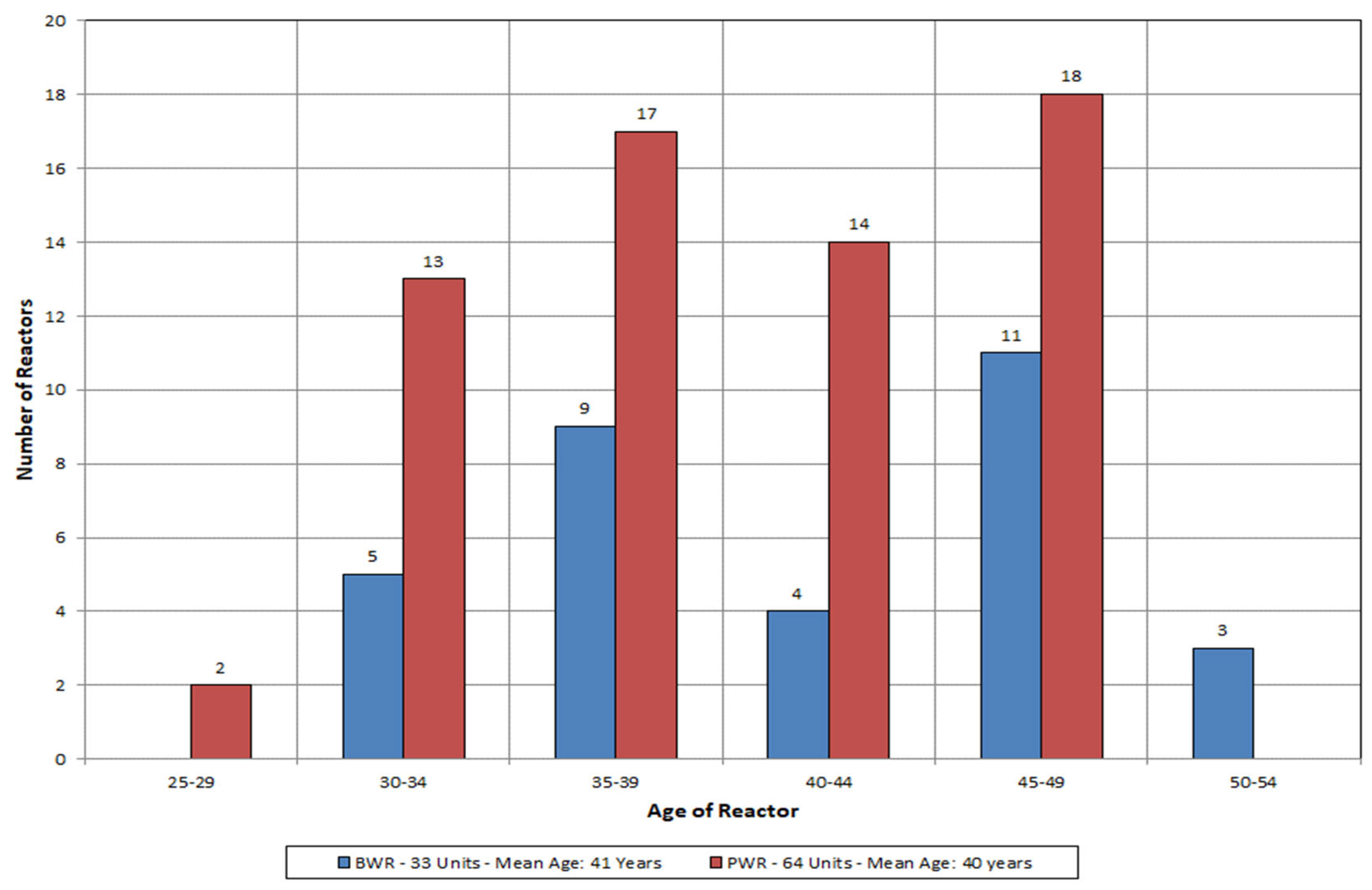
  • Aging plant fleet and accumulation of pipe damage from degradation mechanisms. As shown in Figure 3 below, of the current U.S. plant fleet, 50 reactor units have entered an extended period of operation (i.e., ≥40 years).
  • New operating experience data. The database that is the source of the pipe failure rate estimates is continuously updated and maintained. The overall body of service experience data has been substantially expanded since the first EPRI ‘pipe rupture frequency’ report was issued in 2006.
  • Enhancements in reliability and integrity management. The plant license renewal initiatives together with applications of non-destructive examination (NDE) techniques and inspection qualification processes have evolved since the first EPRI ‘pipe rupture frequency report’ was issued. Embedded in the operating experience data are effects of NDE, replacement of pipe segments, improvements to leak tests and inspections, and changes in the reporting of pipe failures.
Age-dependent pipe failure rate estimation can be performed according to different analysis strategies to obtain piping reliability parameters as a function of the age of an affected pipe section at the time of its observed failure, age of the plant, or as a function of the temporal changes in the piping operating experience. Trends in pipe failure rates are influenced by physical changes to the structural integrity (e.g., pipe wall loss) due to degradation mechanisms, changes in reporting routines, design changes (e.g., replacing original carbon steel piping with piping made of corrosion-resistant material), and changes in reliability and integrity management (i.e., in-service inspection).

4.2. Aging Factor Model

The treatment of aging using the aging factor model was applied to the service water pipe system and the fire protection pipe system cases in the scope of systems covered in the Reference [1] report. For the remaining cases described in Reference [1], there was insufficient data to identify statistically significant aging trends. Aging factors were truncated at 60 years to avoid over extrapolation beyond what the service data can support. Guidance is provided in the roadmap section of the report for applying the aging factors to each of the mean flood frequency metrics presented in the report. The user has the option of using the lookup tables described in the previous section or using the formulas based on system specific parameters for applying the following Equation (2).
Aging factors are calculated for the fire protection and service water systems using the following approach:
  • For each calculation case (system, pipe diameter, and type of raw water for the service water system), organize the pipe failure population by time period in which a failure was observed:
    Pool data by pipe size for each of the three cases:
    BWR ASME Class 3 Service Water;
    PWR ASME Class 3 Service Water;
    Fire Protection (all failure modes).
  • Segment data into time intervals; because of the size of the pipe failure populations for the two system groups, different approaches were used in the processing the data:
    The service water pipe failure population was fairly evenly spread across the five decades, 1971 to 2020, so the failure population was placed in ten 5-year bins.
    The bulk of the fire protection failure population was primarily from the 1990–2020 time period, so the failure population was placed in five 10-year bins.
  • For each case and time interval, determine the average age of the piping systems that produced the pipe failures.
  • Using the Constrained Noninformative Distribution (CNID) method [17] with a prior failure rate of 2.0 × 10⁻⁵ per ROY-ft based on the generic data in Reference [11], calculate the temporal failure as the average failure rate for that interval. This is accomplished by performing a Bayes’ update of the failure rate using the number of observed pipe failures and reactor operating years and feet of piping for that time interval as the evidence to update the prior. The prior failure rate is reduced to 2 × 10⁻⁶ per ROY-ft in the first interval to prevent too much influence by the prior to the zero failure cases.
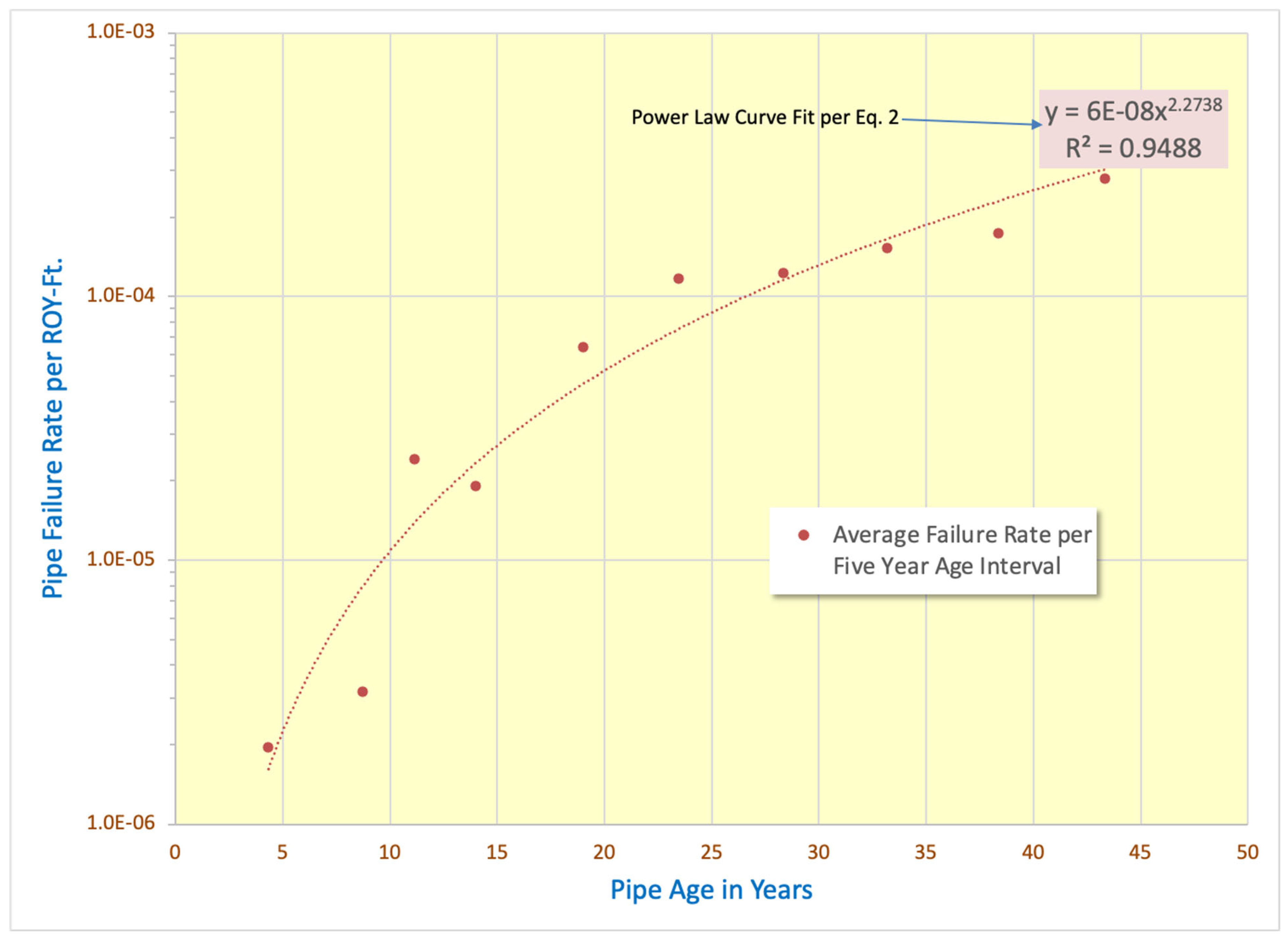
  • Using Microsoft® Excel, plot a line of best-fit through the scatter plots of failure rate vs. plant age (Figure 4), resulting in a log-linear power model with scale and shape factors. For each respective calculation case, the age factor Ait is determined from the following:
A 1 t = a i t b i λ i
where
A i t = Aging factor at pipe age t for component i defined by system, design, or code class and pipe size;
a i = Scale parameter for component i;
b i = Shape parameter for component i;
λ i = Average pipe failure rate for component i .
The result for one case, BWR Class 3 service water piping in the 2″ to 4″ size range, is illustrated in Figure 4. This process was repeated for all the service water and fire protection system cases in Table 1.

4.3. Review of Aging Factor Approach

The entire data analysis documented in Reference [1] was independently reviewed by the John Garrick Risk Sciences Institute at UCLA, including the method of calculating age factors. A variety of data pooling strategies, data window truncation studies, and different curve-fit models were investigated to understand the uncertainty and sensitivity to modeling assumptions of the aging model. The resultant aging factor model and alternative pooling strategies were peer reviewed by members of the team not involved with the pipe failure rate estimations. This review examined questions regarding the approach to aging factor estimation. Specifically, the data pooling strategies. Factors considered include the following:
  • Completeness of input data over time (i.e., failure reporting)
  • Understanding the “outliers” in the failure population and how to handle in trend analysis.
  • Data pooling strategies to overcome sparsity of data while accounting for the following:
    Influence of water source (sea, lake, river);
    Pipe size;
    Influence of plant type;
    Influence of time interval (5 yr v. 10 yr bins);
    Trend model selection;
    Assumptions on data window.
The failure model is capable of producing failure rates depending on many factors including system, pipe size, pipe code class, pipe materials, reactor type, and nature of operating fluid (water type, pressure, temperature, etc.). To explore the impact of data pooling strategies on confirmation of aging, trending model selection, and optimum statistical fit, a large number of cases were analyzed. As described in that table, variable plant type, pipe size, and water source were considered. In the table, Groups 1, 2, and 3 were analyzed using 10 × 5 yr time intervals for binning failure data by age (referred to as Model 1), while Group 4 is a variant of Group 2 with failures rates binned into 5 × 10 yr time intervals (Model 2).
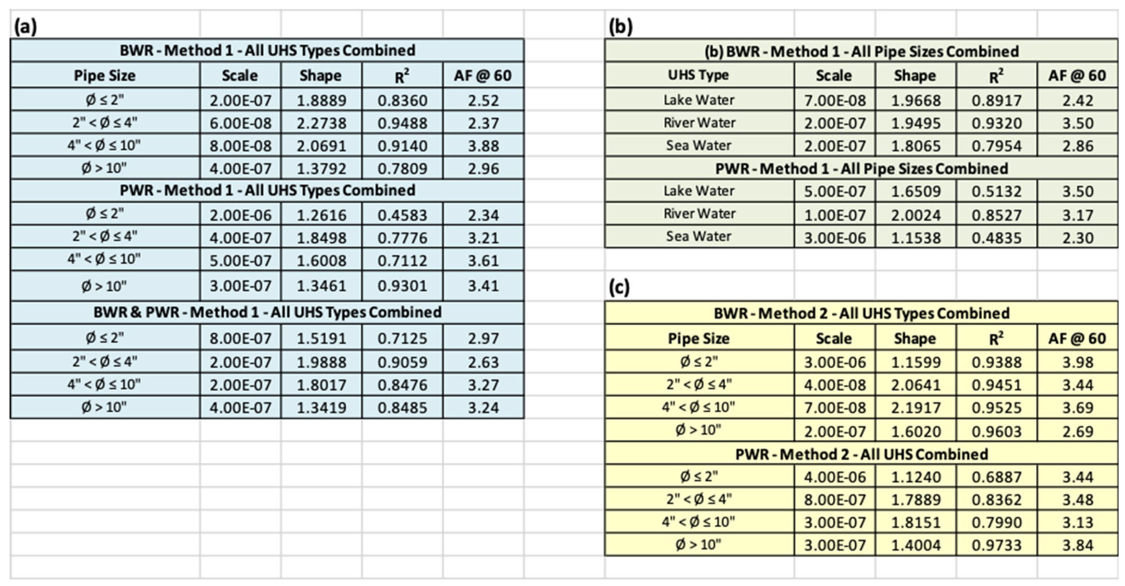
All cases showed an increasing failure rate trend in the form of the fitted curve, subject to statistical variations of the data points, similar to that in Figure 4. The resulting power law model parameters and corresponding R2 statistical test values for model fitting for Analysis Groups 2, 3, and 4 are shown in Figure 5a–c. The Figures show the model projections of AF at Age 60.
While based on engineering arguments in favor of separating the failure data by plant type, water source, and pipe size, one would lean towards the base case (analysis Group 1), the R2 values for some of the 24 cases were poor.
Among the pooling strategies, cases that produced the best balance between statistical and engineering considerations are those listed in Figure 5a where data are pooled only by water source, keeping plant type and pipe size as variables. For this case, the 2″ PWR piping showed a somewhat weak correlation; the AF for this case was accepted based on a review of the underlying factors and engineering judgement based on understanding the overall data trends.
In addition to the analysis groups enumerated in Figure 5, additional calculation cases were run considering different data window truncations as well as different curve fit models. These are described in Table 3. Across all analysis cases, the aging factors were generally in the range of 2–4. There were a few cases where the aging factor for a specific pipe case(s) exceeded that, but in those cases, the statistical significance of the trends was found to be low and/or the model was considered an inappropriate fit (i.e., the exponential curve fit). The scope of the aging factors was limited to a plant age range of 60 yrs to avoid over-extrapolation of the models beyond what the service data can support.
The peer review of the aging factor approach concludes that the approach is reasonable and consistent with typical PRA data analysis practices. Specifically, the method achieves the following:
  • It has clearly defined scope and limitations;
  • It is based on the most relevant data and uses appropriate analysis methods;
  • It has sufficiently considered the range of modeling assumptions, and appropriately applied a balance of statistical significance and engineering judgement;
  • The final results are consistent with expectations based on review of the experience data;
  • The approach, results, and expected application of the results are clearly documented in the final report [1].
Aging factors were developed for all the pipe cases identified in Table 1. An example for BWR Class 3 carbon steel service water piping is shown in Table 4.

5. Evaluation of Integrity Management Factor

5.1. Markov Model Overview

The use of the Markov model to adjust pipe failure rates for different crack and leak surveillance strategies was introduced in previous revisions of this report and has been retained in the Revision 5 update.
The reliability characteristics of piping systems are potentially influenced by various surveillance programs, including leak detection systems, system leak and pressure tests, and in-service inspections involving visual and volumetric examinations of the piping system components. When service data are applied, the surveillance programs that were implemented on the systems in the database might have influenced the piping reliability; however, it is not possible to isolate their quantitative impacts on failure rates. Furthermore, these surveillance programs might be different from those being considered for the pipe whose reliability characteristics are being estimated or predicted, especially if the plant in question has employed more aggressive surveillance strategies than those typical of standard industry practice.
The influence of surveillance strategies is accounted for in the pipe reliability model by the integrity management factor Iik shown in Equation (1). This factor is quantified using the Markov model for evaluating the effectiveness of reliability and integrity management (RIM) strategies [9]. As was the case with the Bayesian uncertainty treatment described in the previous section, the Markov model was originally developed for RI-ISI evaluations for LWR piping systems and approved by the NRC for use in these applications [13].
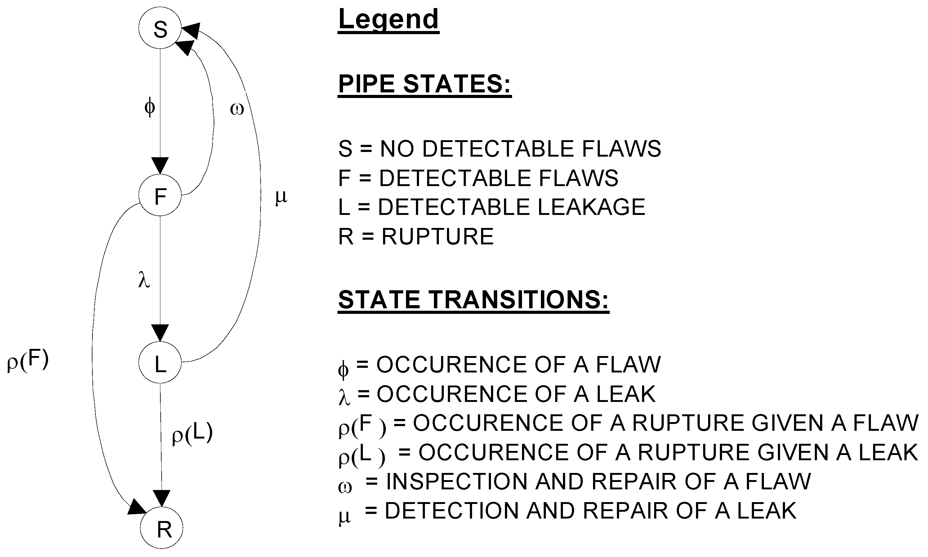
The Markov model for this application is shown in Figure 6. This model is applied to each component in a piping system, including the areas of the pipe around welds and in other locations that might be subject to a degradation mechanism and be the target of a RIM strategy to detect leaks, perform NDE for flaws, or a combination of these. Each location is assigned four possible states to represent no degradation, degradation with detectable flaws, leak, and rupture. Transition rates between states are assigned to model the damage mechanisms producing each failure mode along with two opportunities to detect damage and repair the pipe prior to its rupture. One of these represents the process of detecting flaws through NDE and subsequent repair if damage is found; the other represents the leak inspection/detection and repair process. The model offers the capability of modeling degradation that obeys a “leak before break” failure process as well as mechanisms that produce pipe rupture without a prior leak warning. The purpose of this model is to predict the influence of ISI exams and leak detection strategies on reducing the pipe rupture frequency.
The repair rates m and w are estimated with the help of two simple models. For the flaw repair rate w, the model of Equation (3) is used:
ω = P I P F D ( T F I + T R )
where
  • PI = probability that a piping element with a flaw will be inspected per inspection interval. When locations for the inspection are fixed, this term is either 0 or 1, depending on whether the pipe segment is inspected.
This probability of inspection term is conditioned on (that is, assumes the occurrence of one or more flaws in the piping element being modeled) a weld or piping segment with similar damage mechanism potential. This is true because this Markov model transition rate, w, is applied only to the initial state of a flaw. The model assumes that the flaw is severe enough to cause a need for repair or replacement if the NDE is successful in identifying it.
  • PFD = probability that a flaw will be detected given that this segment is inspected. This parameter is related to the reliability of NDE inspection and is a conditional probability given that the location being inspected has a flaw that meets the criteria for repair according to the ASME code.
  • TFI = mean time between inspections for flaws (inspection interval).
  • TR = mean time to repair when detected. There is an assumption in this model that any significant flaw that is detected will be repaired. Because TFI, which is measured in years, is normally much greater than TR which is measured in hours, the results of applying the Markov model are not sensitive to assumptions regarding TR.
Similarly, estimates of the repair rate for leaks can be estimated according to Equation (4):
μ = P L D ( T L I + T R )
where
  • PLD = probability that the leak in the segment will be detected per inspection.
  • TLI = mean time between inspections for leaks.
  • TR = as defined above but for full power applications. This time should be the minimum of the actual repair time and the time associated with any technical specification limiting condition for operation (LCO) if the leak rate exceeds technical specification requirements.
Opportunities for leak detection are highly dependent on the system in which the leak occurs as well as the specific location and size of the leak. Some leaks might be detected only upon periodic leak testing, which might occur less often as required to meet ASME rules for different classes of pipe according to ASME Section XI and other requirements for leak testing.
An important observation about this leak repair term m in comparison to the flaw repair term w is that for most leaks the detection possibilities are not normally limited to some predetermined population of welds that are inspected. However, leak testing often provides an opportunity to inspect all locations system wide. Therefore, given a leak of significant magnitude anywhere in the system, the probability of leak detection tends to be high. For locations that are not subjected to an inspection the flaw repair rate term, w, is equal to zero. In addition, the time between successive inspections for leaks tends to be much shorter than for volumetric examination of welds with virtually instantaneous detection in cases in which the leak would trigger an alarm in the control room. Therefore, the Markov model provides the capability to account for the leak-before-break principle. The extent to which this principle contributes to reducing the probability of a rupture is a function only of the relative values of the Markov model transition rates.
The Markov model and the pipe failure model it is used with have been extensively reviewed, including reviews performed by the U.S. Nuclear Regulatory Commission and Los Alamos National Laboratory for use in the EPRI Risk Informed Inservice Inspection Program [12,13]. In the NRC’s safety evaluation of the program, the following findings are stated. The reference numbers in the quoted text have been changed to refer to the reference list in this paper:
Technical reviews of the Markov model have been performed by the staff, a staff contractor (Ref. [12]), and by independent peer reviewers for EPRI. These efforts provided a detailed review of the model and its ability to support the proposed licensing application. The conclusion of the reviews is that the proposed four-state Markov model as described in EPRI-TR-110161 is both sound and appropriate as a first-order model of pipe rupture. The staff adopts the analysis of the Markov model and the Bayesian updating set forth in the contractor report (Ref. [8]). The contractor report is available in the Commission’s Public Document Room, which is located in the Gelman Building at 212 L St, N.W., Washington, D.C., 20003, under accession number 9909300045. Based on that analysis, the staff finds that the model can be used as a basis for the estimation of pipe rupture frequencies to be used instead of the bounding pipe failure frequencies in support of the change in risk estimates as part of an application that uses the EPRI RI-ISI methodology.

5.2. How the Markov Model Is Used in This Study

The Markov model is used to set up a set of linear coupled differential equations whose solution provides the time-dependent probabilities of occupying each of the four states of the model. This solution is used to derive time-dependent hazard rates for the model. A different solution is obtained for each rupture mode (break size). As described more fully in [9], a closed form analytical solution for the time-dependent rupture frequencies as a function of all of the input parameters is obtained, and these solutions are entered into a Microsoft Excel spreadsheet. The input parameters to quantify the model include failure rates and rupture frequencies derived from service data as well as parameters that describe the RIM program. These parameters and the way they are applied in this report are defined in Table 5. The application of the Markov model to adjust the pipe failure rates to account for alternative RIM strategies is described in the next section.
There is a cause-and-effect loop that must be broken to perform this application. The failure rates and rupture frequencies derived from service experience assume that the components will be subjected to a RIM program that is the same as or similar to that which the piping in the LWR service data has historically been subjected to. These rates are also derived from a population of reactors that has experienced, on average, decades of commercial operation. In the LWR service data, the RIM program is primarily dictated by ASME Section XI requirements for ISI, related requirements for leak testing or pressure testing, and augmented or owner-defined inspection programs for specific damage mechanisms not addressed in Section XI. This cause-and-effect loop is broken using the following logic.
The integrity management factor in Equation (1) is derived from the Markov model using Equation (5):
I i x = h i x t h i B A S E t
where
  • Iix(t) = integrity management factor for component i for RIM strategy x at piping system t. As shown in this equation, this factor can be expressed as a product of separate integrity management and piping system factors. The RIM strategy includes a specification of how often leak tests and inspections and NDE are performed on the piping system component and how effective they are.
  • hix(t) = hazard rate (time-dependent rupture mode frequency) for component I at piping system t and RIM strategy x. This is determined from the solution of the ordinary differential equations that describe the Markov model as explained more fully below. The piping system is set at the average piping system in the plant population responsible for the failure rate and conditional rupture frequency estimates.
  • hiBASE(t) = hazard rate (time-dependent rupture mode frequency) for component i at piping system of t and RIM strategy corresponding to an “average” component in the service data.
Two distinct applications of the Markov model are employed in this study:
  • Adjusting service data to derive additional piping cases: To estimate the failure rates and rupture frequencies for non-safety-grade SW piping using data from safety grade piping which has stricter integrity management requirements. In this case, failure rates and rupture frequencies for ASME Class 3 SW piping are derived from the service data; Equation (5) is then evaluated for the RIM strategy of no leak testing and no ISI.
  • Accounting for plant-specific integrity management enhancements: In the second application, additional RIM strategies are evaluated that could be used to reduce the failure rates and rupture frequencies below those reflected in the service data by conducting more inspections and tests than are reflected in the service data.

5.3. Specific RIM Strategies Used in Flood Frequency Data

To facilitate the practical application of the Markov model and to address industry requests for additional guidance to use this methodology in practical application, a set of “standardized” RIM strategies are introduced. There are five basic RIM strategies defined for this purpose including the following:

5.3.1. RIM-0 Standard Industry Practice

The integrity management factor for this case is 1.0. This is the default case when there is no special integrity management factor applied to specific pipe segments identified in the IFPRA for which the flood frequencies are to be estimated.

5.3.2. RIM-1 Enhanced Leak Testing

The integrity management factor for this case is less than 1 and is dependent on the pipe case, EBS, and flood frequency metric. This applies when there are enhanced leak testing strategies applied to specific pipe segments identified in the IFPRA.

5.3.3. RIM-2 Robust Leak Testing

The integrity management factor for this case is less than 1, less than that for RIM-1, and is dependent on the pipe case, EBS, and flood frequency metric. This applies when there are robust leak testing strategies applied to specific pipe segments identified in the IFPRA.

5.3.4. RIM-3 Robust Leak Testing and Enhanced NDE

The integrity management factor for this case is less than 1, less than that for RIM-2, and is dependent on the pipe case, EBS, and flood frequency metric. This applies when there are robust leak testing and enhanced NDE strategies applied to specific pipe segments identified in the IFPRA.

5.3.5. RIM-4 Robust Leak Testing and Robust NDE

The integrity management factor for this case is less than 1, less than that for RIM-3, and is dependent on the pipe case, EBS, and flood frequency metric. This applies when there are robust leak testing and robust NDE strategies applied to specific pipe segments identified in the IFPRA.
Definitions of what is meant by “enhanced” and “robust” are summarized in Table 6. Integrity management factors were originally developed to support the EPRI Risk-Informed Inservice Inspection program and have been applied in several industry IFPRAs to reduce the frequency of risk-significant flood-induced accident sequences. For each of these RIM strategies, a set of integrity management factors was developed for each flood frequency metric and each pipe case for the service water and fire protection system piping in the scope of the study. Examples of integrity management factors for 24″ pipe in BWR Class 3 service water systems using carbon steel are listed in Table 7.

6. Roadmap for Selection and Application of Flood Frequency Parameters

Given the scope of pipe flood frequency cases, flood frequency modifiers for aging and integrity management, and flood frequency metrics, it was decided in Revision 5 to produce the results for users in the form of Excel spreadsheets, rather than report tables. The appendices of [1] are listed below. The baseline flood frequency metrics are listed in Appendixes A, B, and D of [1]. Adjustment factors for aging and enhanced RIM strategies are provided in Appendix C of [1] for service water and fire protection systems. Appendix E of [1] contains flood frequency data formatted for input to the EPRI FRANX software Version 11 [16], which can be used to assist EPRI members in the development of data for internal flooding PRAs.
  • Appendix A: Service Water System Data Tables
  • Appendix B: Fire Protection System Data Tables
  • Appendix C: Service Water and Fire Protection Systems Adjustment Factors Data Tables
  • Appendix D: Other Water Systems Data Tables
  • Appendix E: FRANX Files
  • Appendix F: Internal Flooding Event Database
  • Appendix G: Documentation of Independent Review
  • Appendix H: PIPExp Database
Flood frequencies were generally derived based on average system performance from 1970 through 2020. The data window for feedwater, condensate, and steam system data was truncated to screen out early service experience before industry initiatives to reduce the impacts of flow-accelerated corrosion were implemented; service experience before 1989 for FAC-susceptible piping was not used for those systems. The roadmap for selection and application of flood frequency data for the service water and fire protection system cases is shown in Figure 7. The boxes refer to section numbers in the Reference [1]. The roadmap section provides guidance on the selection of flood frequency base values, adjustment factors, and additional guidance for how to address systems with different pipe sizes and system pressures.
Figure 7. Roadmap for selection and use of EPRI flood frequencies and adjustment factors. Reproduced with permission from [1]; published by EPRI, 2023. The formats used to present the results of the basic flood frequency metrics in the Excel spreadsheets are shown in Figure 8 and Figure 9 for the cumulative break frequency and flood rate interval frequency metrics, respectively.
Jne 06 00037 g007
Figure 8. Cumulative break frequency (EBS and flood rate) metric. Reproduced with permission from [1]; published by EPRI, 2023.
Jne 06 00037 g008
Figure 9. Flood rate interval metrics (flood rate interval and flood mode). Reproduced with permission from [1]; published by EPRI, 2023.
Jne 06 00037 g009

7. Trends in Flood Frequency Estimates

While failure rates generally increased due to aging, with refinement of the conditional rupture probability models, the individual flood mode frequencies exhibited both reductions and increases. Trends in the service water system flood frequency cases when comparing the results produced in Revision 3 [2] and Revision 5 [1] of the pipe report series are shown in Figure 10. As seen in this figure, which compares flood frequencies in different pipe sizes, flood modes, reactor types, and service water sources, some flood frequencies were found to increase and others were found to decrease. These comparisons were made on the base flood frequencies without the application of aging factors. In general, the increases reflect the effects of aging, and the decreases reflect the impact of methodology improvements that offset the effects of aging.
Increases in larger flood rates were generally driven by the occurrence of actual breaks in the more recent data. More detail on differences can be found in the chapters for each individual system as discussed in Sections 4–8 of Reference [1]. The overall point is that even though we have aging, overall, due to data improvements and improvements to the methodology, some failure rates and flood mode frequencies have increased, while others have decreased. In addition, the refinements in the methodology are viewed as producing more realistic estimate of flood frequencies to support technically sound internal flooding PRAs.

8. Summary and Conclusions

Revision 5 of the EPRI report on pipe rupture frequencies has documented many advancements to improve the capabilities of internal flooding PRAs as well as improved guidance for selection and use of flood initiating event data. These advancements are summarized in the following.
  • Compared with the previous revision in Reference [2] the service experience with piping systems that have been used has been expanded from 2010 to 2020.
  • A wider scope of piping systems is now supported in terms of piping system design codes, pipe materials, and pipe sizes. These cases demonstrate the advantages in replacing carbon steel pipe with corrosion-resistant materials that reduce susceptibility to corrosion-related damage mechanisms that are present in raw water systems and high-energy piping.
  • A larger set of flood frequency metrics has been included to facilitate use of the pipe failure data in performing internal flooding and high-energy line break PRAs.
  • The flood frequencies provided address the aging of piping systems associated with degradation mechanisms and trends in reporting. This is the first time a generic database developed to support industry PRAs has explicitly addressed the impact of aging on component failure rates.
  • The ability to adjust the flood frequencies to account for enhanced integrity management strategies has been improved and is more easily applied. As demonstrated in the development of risk-informed inservice inspection programs, enhancements to the procedures for inspection of leaks and performance of non-destructive examinations can greatly reduce the frequency of pipe ruptures.

Author Contributions

Conceptualization, K.N.F. and B.O.Y.L.; methodology, K.N.F. and B.O.Y.L.; software, K.N.F. and M.P.; validation, A.M., W.C. and M.P.; formal analysis, K.N.F., B.O.Y.L. and A.M.; investigation, B.O.Y.L.; resources, M.P.; data curation, W.C. and A.M.; writing—original draft preparation, K.N.F.; writing—review and editing, K.N.F., B.O.Y.L., W.C., A.M. and M.P.; visualization, M.P.; supervision, M.P.; project administration, M.P.; funding acquisition, M.P. All authors have read and agreed to the published version of the manuscript.

Funding

This work was funded by the Electric Power Research Institute.

Data Availability Statement

The data presented in this paper are developed in Reference [1] which can be obtained from EPRI for the purchase of a license.

Conflicts of Interest

Karl Fleming was employed by KNF Consulting Services LLC and Bengt Lydell was employed by Sigma Phase Inc. Mary Presley was employed by the Electric Power Research Institute. The authors declare that this study received funding from Electric Power Research Institute. The funder had the following involvement with the study: “review and interpretation of the findings of the project”.

References

  1. Pipe Rupture Frequencies for Internal Flooding Probabilistic Risk Assessments, Revision 5; EPRI: Palo Alto, CA, USA, 2023; p. 3002024904.
  2. Pipe Rupture Frequencies for Internal Flooding PRAs, Revision 3; EPRI: Palo Alto, CA, USA, 2013; p. 3002000079.
  3. Piping System Failure Rates for Corrosion Resistant Service Water Piping; EPRI: Palo Alto, CA, USA, 2014; p. 3002002787.
  4. Pipe Rupture Frequencies for Internal Flooding PRAs, Technical Update for High Energy Line Piping; EPRI: Palo Alto, CA, USA, 2017; p. 3002009993.
  5. Guidelines for Performance of Internal Flooding Probabilistic Risk Assessment; EPRI: Palo Alto, CA, USA, 2009; p. 1019194.
  6. ASME/ANS RA-S-1.1-2022; Standard for Level 1/Large Early Release Frequency Probabilistic Risk Assessment for Nuclear Power Plant Applications. American Society of Mechanical Engineers and American Nuclear Society: New York, NY, USA, 2022.
  7. Fleming, K.N.; Lydell, B.O.Y. Database Development and Uncertainty Treatment for Estimating Pipe Failure Rates and Rupture Frequencies. Reliab. Eng. Syst. Saf. 2004, 86, 227–246. [Google Scholar] [CrossRef]
  8. Revised Risk-Informed In-Service Inspection Procedure; Rev. B-A; EPRI: Palo Alto, CA, USA, 1999; p. TR-112657.
  9. Fleming, K.N. Markov Models for Evaluating Risk Informed In-Service Inspection Strategies for Nuclear Power Plant Piping Systems. Reliab. Eng. Syst. Saf. 2004, 83, 27–45. [Google Scholar] [CrossRef]
  10. Piping System Reliability and Failure Rate Estimation Models for Use in Risk-Informed In-Service Inspection Applications; EPRI: Palo Alto, CA, USA, 1998; p. TR-110161.
  11. Piping System Failure Rates and Rupture Frequencies for Use in Risk-Informed In-Service Inspection Applications; EPRI: Palo Alto, CA, USA, 1999; p. TR-111880.
  12. Martz, H. Final (Revised) Review of the EPRI-Proposed Markov Modeling/Bayesian Methodology for Use in Risk-Informed Inservice Inspection of Piping in Commercial Nuclear Power Plants; Los Alamos National Laboratory: Los Alamos, NM, USA, 1999; p. TSA-1/999-164. [Google Scholar]
  13. U.S. Nuclear Regulatory Commission. Safety Evaluation Report Related to Revised Risk-Informed In-Service Inspection Evaluation Procedure; Rev. B; EPRI: Washington, DC, USA, 1999; p. TR-112657, This is included in Reference [8]. [Google Scholar]
  14. Poloski, J.P.; Marksberry, D.; Atwood, U.C. Rates of Initiating Events at U.S. Nuclear Power Plants: 1987–1995; NUREG/CR-5750; U.S. Nuclear Regulatory Commission: Washington, DC, USA, 1999.
  15. U.S. Nuclear Regulatory Commission. Estimating Loss-of-Coolant Accident (LOCA) Frequencies Through the Elicitation Process; NUREG-1829; U.S. Nuclear Regulatory Commission: Washington, DC, USA, 2008.
  16. FRANX Version 11 Packaged in Phoenix Architect Version 2.0a; EPRI: Palo Alto, CA, USA, 2023; p. 3002026269.
  17. U.S. Nuclear Regulatory Commission. Handbook for Parameter Estimation for Probabilistic Risk Assessment; NUREG/CR-6823; U.S. Nuclear Regulatory Commission: Washington, DC, USA, 2003.
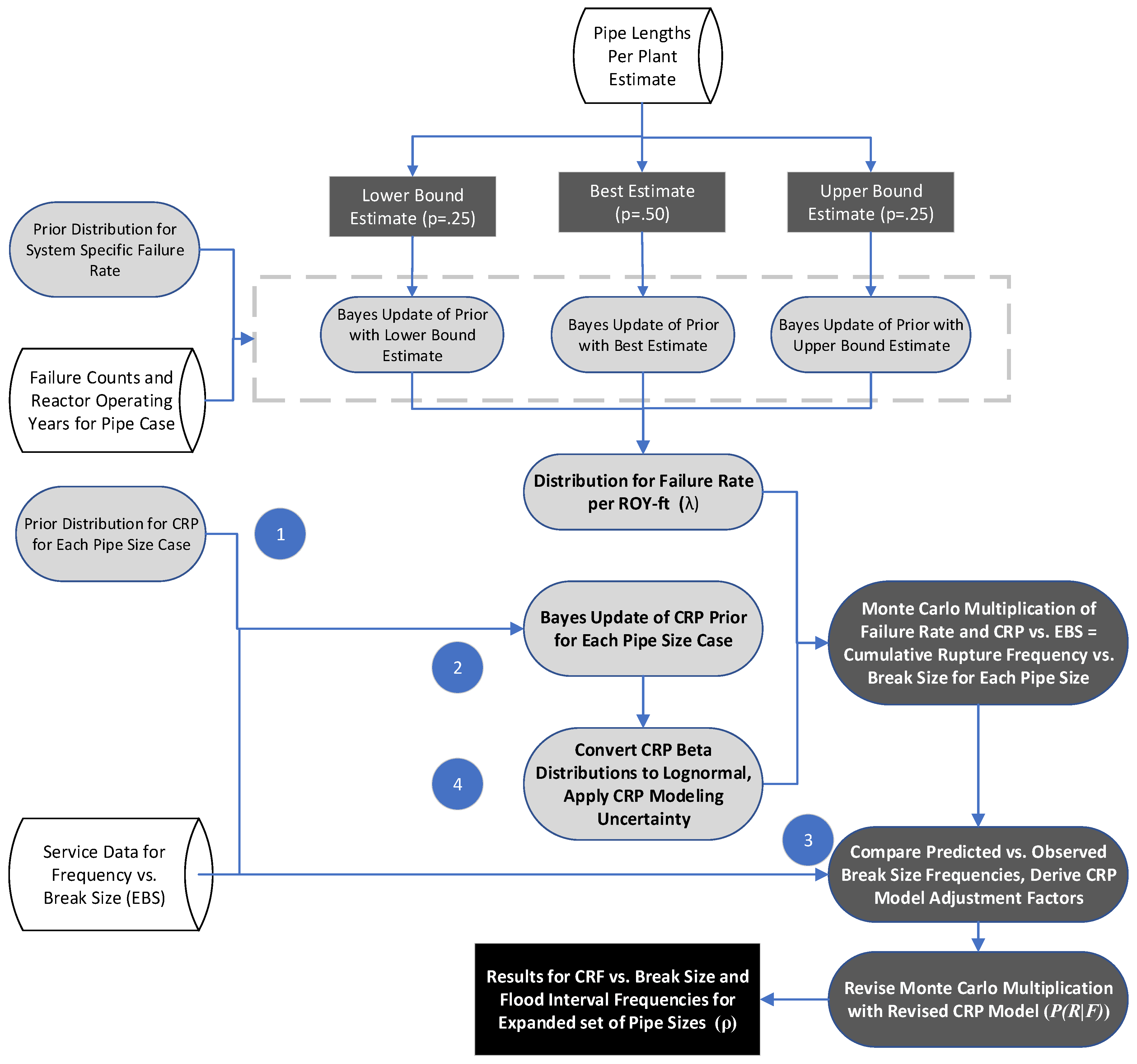
Figure 1. Pipe rupture frequency calculation process. Reproduced with permission from [1]; published by EPRI, 2023. Legend: 1. Develop Prior Distribution, 2. Bayes’ Update Stage 1, 3 Bayes’ Update Stage 2, 4. Apply Modeling Uncertainty.
Jne 06 00037 g001
Figure 2. Evolution of the U.S. service water failure rates by decade 1970–2020. Adapted with permission from [1]; published by EPRI, 2023.
Jne 06 00037 g002
Figure 3. Age of the U.S. nuclear plant fleet at the end of 2020. Reproduced with permission from [1]; published by EPRI, 2023.
Jne 06 00037 g003
Figure 4. Power law curve fit to failure rate estimates—BWR Class 3 SW 2 to 4 in pipe. Adapted with permission from [1]; published by EPRI, 2023.
Jne 06 00037 g004
Figure 5. Power law model parameters and corresponding R2 statistical test values for model fitting for BWR and PWR service water systems. Reproduced with permission from [1]; published by EPRI, 2023. (a) shows cases with all ultimate heat sink (UHS) types combined with data binned in 10 × 5 year intervals; (b) shows cases with all pipe sizes combined with data binned in 10 × 5 year intervals; (c) shows cases with all UHS types combined and data binned in 5 × 10 year intervals.
Jne 06 00037 g005
Figure 6. Markov model for predicting the influences of leak detection and pipe inspections on pipe rupture frequencies. Reproduced with permission from [1]; published by EPRI, 2023.
Jne 06 00037 g006
Figure 10. Comparison of service water flood mode frequencies—all cases. Reproduced with permission from [1]; published by EPRI, 2023. (a) provides this comparison; (b) explains the codes used in (a).
Jne 06 00037 g010
Table 1. Comparison of piping system scope between Revision 5 [1] and Revision 3 [2] of the EPRI Flood Frequency Reports. Reproduced with permission from [1]; published by EPRI, 2023.
System 1Reactor Type CasesType CasesPipe Class CasesNominal Pipe Size (in.) Cases
Service waterBWR, PWRLake, River, SeaASME Class 3 Carbon Steel, ASME Class 3 Corrosion-Resistant Steel 2, ASME B31.1 Carbon Steel (non-safety)2, 3, 4, 6, 10, 12, 16, 18, 20, 24
Fire protectionAllWith and Without WH protectionNon-safety4, 6, 8, 10, 12, 24
SIR outside containmentAllN/AASME Class 34, 6, 10, 14, 24
CCW and CST 3AllN/ANon-safety4, 6, 10, 14, 24
FWC outside containmentBWR, PWR, AllStainless steel 4, Carbon steel (FAC susceptible)Non-safety3, 4, 6, 10, 18, 24, 42
HP steam outside containmentBWR, PWR, AllStainless steel 4, Carbon steelNon-safety3, 4, 6, 10, 18, 24, 42
LP and EXT steam 5BWR, PWR, AllStainless steel 4, Carbon steelNon-safety3, 4, 6, 10, 18, 24, 42
Circulating waterAllPiping, Expansion joint, MOV bodyNon-safety726
Plant level floodsAllAllAllAll
1 System abbreviations: CCW = component cooling water, CST = condensate storage tank, SIR = safety injection and recirculation, FWC = feedwater and condensate; HP = high pressure; LP = low pressure; EXT = extraction steam; WH = water hammer. 2 Corrosion-resistant SW cases were originally provided in a technical update [3] to Revision 3 [2]. 3 Data include piping associated with CST but not failure of the tank itself. 4 Flow-accelerated corrosion (FAC)-resistant piping was added to this revision. 5 In Revision 3, separate results were presented for EXT and LP steam; in this Revision, they are combined. 6 In Revision 3, the pipe size for Circulating Water pipe was listed as >24″; however, this piping is actually 72″ in size. No change here, just a clarification of the correct size.
Table 2. Analysis steps and treatment of uncertainties in the application of the pipe failure model. Adapted with permission from [1]; published by EPRI, 2023.
Analysis StepUncertainty Treatment
1. Establish Prior Distribution for failure rate.The Constrained Non-Informative Distribution method of Reference [17] is used to characterize uncertainty in the prior. The mean value is anchored to system specific pipe failure rates developed for EPRI RISI program in Reference [8].
2. Collect failure data for each analysis case and pipe size.Develop point estimate of pipe failure rate for each component i.
li = Number of failures/(pipe length per plant x reactor operating years).
3. Estimates of pipe lengths per plant for representative sample of plants.
4. Calculate reactor operating years of experience relevant to pipe analysis case.
5. Characterize uncertainty in the estimated pipe lengths per plant [10,13].Perform 3 Bayes’ updates of the CNID prior distribution for the failure rate li for each component i; one for the best estimate of pipe length, one assuming pipe length is 50% higher, and one assuming pipe length is 50% lower. This yields 3 Gamma distributions for li, one for each estimate of pipe length per plant.
Using engineering judgment, assign a 50% probability that the best estimate of pipe length is the correct value, 25% probability that the lower estimate is correct, and 25% that the upper estimate is correct.
Using Monte Carlo simulation, calculate a mixture distribution combining the above Gamma distribution using the stated probability weights. This yields one uncertainty distribution of li for each component i.
6. Develop prior distribution for the conditional probability of rupture, P i R x F .Use engineering judgement based on insights from analysis of service data, results of probabilistic fracture mechanics analyses, and expert elicitation to estimate the probabilities for discrete levels of break size. Use CNID method using the BETA distribution to characterize the prior distributions for each break size using these probabilities as mean values.
7. Collect industry data on the frequency of leaks and floods with different flood rates applicable to component i. Convert to equivalent break sizes.Perform Bayes update of the prior distributions to obtain Bayes’ posterior distributions for each conditional probability of rupture size. This yields new conjugate BETA distributions for each P i R x F .
8. Apply adjustment factors to value of P i R x F to ensure that that industry wide flood frequencies predicted by the pipe failure model agree with the observed industry data. [New to this revision].Adjustment factors are developed by comparing the predicted frequencies of different break size against the observed frequencies from the service data. The former are obtained multiplying the mean values of P i R x F and λ i times the pipe component exposure to obtain the predicted industry wide frequency of leaks of different sizes. Adjustment factors are calculated to make the predictions consistent with the industry data. These are used to modify the P i R x F values to ensure agreement.
9. Apply modeling uncertainty to account for the modeling assumption that each pipe failure is a precursor to a more severe pipe rupture.Convert Bayes’ posterior BETA distributions from Step 7 to lognormal distribution by matching the mean values and assignment of range factors that increase with decreasing rupture probability.
10. Develop overall uncertainty in the pipe rupture frequency for each value of ρix.Perform Monte Carlo uncertainty analysis to combine the uncertainties in λ i and P i R x F . Fit the resulting distributions to lognormal distributions by matching the means and estimating the range factor (RF) from the Monte Carlo distribution percentiles: RF = SQRT(95%tile/5%tile).
11. Develop flood frequency metrics for use in IFPRA.Convert results from Step 9 into different forms including the following:
  • Cumulative frequency of break size and flood rate;
  • Frequency of flooding in different flood types and flood rate intervals.
12. Develop aging factors, Ait in Equation (1) to convert time-averaged flood frequencies developed in Step 11 to flood frequencies dependent on the pipe age. See Section 4 for details regarding the development and application of aging factors.Estimate the pipe failure rates, λi in Equation (1), by pipe system age; develop correlation between failure rate and pipe age; develop aging factors for each pipe case.
13. Develop integrity management factors, Iix in Equation (1), to account for integrity management strategies for inspections for leaks and flaws in piping system.Use the Markov Model [9] to derive integrity management factors for each pipe case. A factor 1.0 is used when standard industry practices are followed, and values less than 1 are estimated to account for selected strategies where more advanced procedures for detecting for leaks and inspecting for flaws via non-destructive examination are employed. Specific values are associated with the level of rigor of the selected strategy and are defined in [1].
Table 3. Data pooling test cases for service water system.
Analysis GroupFailure Rate VariablesNumber of Analysis Cases
Plant TypePipe SizeUHS Type
0Variable and PooledPooledPooled3
1VariableVariableVariable24
2Variable and PooledVariablePooled12
3Variable and PooledPooledVariable6
4Variable and PooledVariablePooled9
Table 4. BWR service water aging factor multipliers from Appendix C in Reference [1]. Reproduced with permission from [1]; published by EPRI, 2023.
Pipe Age
(Years)
Pipe Size (Inches)
≤2″2″ to 4″4″ to 10″>10″
5 (or less)0.030.010.020.10
100.100.040.100.25
150.210.100.220.44
200.350.190.400.65
250.530.320.630.88
300.730.490.921.14
350.960.691.271.41
401.220.941.681.69
451.511.232.141.99
501.821.562.662.30
552.161.943.242.62
602.522.373.882.96
Table 5. Markov model parameters that vary with RIM strategy. Reproduced with permission from [1]; published by EPRI, 2023.
SymbolDefinitionHow it is Quantified in This Study
PIProbability per inspection interval that the pipe element will be inspectedThis parameter is set to 1 for components assumed to be part of an NDE ISI program and 0 if no inspections are performed.

PFD
Probability per inspection that an existing flaw will be detectedThis parameter is set to 0 for no NDE, 0.5 for enhanced NDE, and 0.9 for robust NDE. This metric is used to provide a degree of confidence that each inspection will identify a detectable flaw according to ASME NDE criteria.
PLDProbability per detection interval that an existing leak will be detectedThis is a function of the reliability of the test being performed for leak detection. This parameter is set to 0.5 for enhanced leak testing and 0.9 for robust leak testing.
TFIFlaw inspection interval; mean time between in-service inspectionsThis parameter is set to 10 years for enhanced NDE and robust NDE.
TLDLeak detection interval; mean time between leak inspectionsLeak inspections are assumed to be performed once per quarter year for enhanced and robust leak testing
TRMean time to repair the piping element given detection of a critical flaw or leakThis parameter is set to 200 h in this study, and the results are not sensitive to this assumption.
lFailure rate for leaksTaken as the failure rate for the smallest equivalent break size (EBS) evaluated in this study—0.32 in; note that this l is somewhat different from that used in Equation (1). This version includes all failures involving leaks, whereas the Equation (1) version includes all failure modes involving repair and replacement, which includes leaks as well as non-leak events.
fOccurrence rate for detectable flawsThis rated is assumed to be a multiple (4) of the total failure rate for the component; consistent with assumptions used for LWR RI-ISI [8]
ρ(F)Rupture frequency given a flawThis is the rupture frequency for each EBS evaluated in this study. The model is evaluated for each EBS in the pipe failure model.
r(L)Rupture frequency given a leakThis rate is assumed to be the rupture frequency given a severe loading condition (for example, water hammer) derived from service data (2 × 10⁻² per year), consistent with assumptions used for LWR RI-ISI evaluations [8].
hBASE(t)Hazard rate for Base RIM strategy at time tHazard rate determined by solving the differential equations for the Markov model with the input parameters as defined in this table set to match the average industry RIM strategies. For ASME Class 3 SW systems, the average component is characterized by 5% of the components being subjected to NDE exams every 10 years for augmented inspection programs 1, the remaining 95% not being subjected to NDE, and 100% of the components being subjected to a system leak test once every refueling outage—which occurs (on average) once every 18 months. Time t is set at the average age of component that was used to develop the failure rate estimates.
hx(t)Hazard rate for variable RIM strategy at time tThe hazard rate is the time dependent rupture frequency of the component with component age. In this version of the hazard rate, the input parameters defined in this table are set to match the parameters of a specific RIM strategy designated as x.
1 For ASME Class 3 piping systems, there is no ASME requirement for periodic NDE; however, service water systems are subjected to augmented inspection programs for specific damage mechanisms such as microbiologically induced corrosion (MIC). The authors estimate that approximately 5% of the industry Class 3 service water piping is subjected to NDE every 10 years.
Table 6. Definition of reliability and integrity management (RIM) strategies. Reproduced with permission from [1]; published by EPRI, 2023.
NameDescriptionElements of Strategy
RIM-0Standard Industry PracticeMaintain current procedures and practice for leak inspections and non-destructive examinations (NDE).
RIM-1Enhanced Leak TestingDevelop written procedure for performance of quarterly leak inspection that identifies all pipe sections for which this strategy is to be implemented. Implementation of the procedures should be capable of performing visual examination of applicable pipe sections that are effective in identifying the presence of leaks. At least 50% of the applicable pipe sections should be accessible for the visual exams to verify leak-tight integrity over the sections of piping system that the integrity management factor is being applied to. If there is water on the floor, source of leakage should be determined. If the applicable pipe section is determined to be leaking, the leak should be repaired or replaced. This strategy is simulated in the Markov model, assuming quarterly leak testing at a 50% probability of finding and repairing a detectable leak and no NDE. Maintain current procedures and practice for leak inspections and non-destructive examinations (NDE) for other pipe sections.
RIM-2Robust Leak TestingDevelop written procedures for performance of quarterly leak inspection that identifies all pipe sections that are applicable to the RIM-2 strategy. Implementation of the procedures should be capable of performing white glove examination, or equivalent, of applicable pipe sections that are effective in identifying the presence of leaks. At least 90% of the applicable pipe sections should be accessible for the visual exams to verify leak-tight integrity over the sections of piping system that the integrity management factor is being applied to 1. If there is water on the floor, source of leakage should be determined. If the applicable pipe section is determined to be leaking, the leak shall be addressed by appropriate repair and replacement. This strategy is simulated in the Markov model, assuming quarterly leak testing at a 90% probability of finding and repairing a detectable leak and no NDE. Maintain current procedures and practice for leak inspections and non-destructive examinations (NDE) for other pipe sections.
RIM-3Robust Leak Testing and Enhanced NDESame leak testing as in RIM-2 with additional 10-year NDE that has the capability to detect a flaw in the applicable pipe sections that exceeds the NDE criteria for repair with a 50% probability of finding a detectable flaw. If the applicable pipe section is determined to be leaking in the quarterly leak inspection or if a flaw exceeding the repair criteria is found in the 10-year NDE, the leak or flaw shall be addressed by appropriate repair and replacement. This strategy is simulated in the Markov model, assuming quarterly leak testing at a 90% probability of finding and repairing a detectable leak combined with a 10-year NDE with a 50% probability of finding and repairing a detectable flaw. Maintain current procedures and practice for leak inspections and non-destructive examinations (NDE) for other pipe sections.
RIM-4Robust Leak Testing and Robust NDESame leak testing as in RIM-3 but with a 10-year NDE that has the capability to detect a flaw in the applicable pipe sections that exceeds the NDE criteria for repair with a 90% probability of finding a detectable flaw. If the applicable pipe section is determined to be leaking in the quarterly leak inspection or if a flaw exceeding the repair criteria is found in the 10-year NDE, the leak or flaw shall be addressed by appropriate repair and replacement. The locations covered by this strategy should be incorporated into the plant’s existing augmented ISI programs. This strategy is simulated in the Markov model, assuming quarterly leak testing at a 90% probability of finding and repairing a detectable leak combined with a 10-year NDE with a 90% probability of finding and repairing a detectable flaw. Maintain current procedures and practice for leak inspections and non-destructive examinations (NDE) for other pipe sections.
Table 7. Integrity management factors for BWR Class 3 SW 24″ pipe for refined flood rate intervals. Reproduced with permission from [1]; published by EPRI, 2023.
Flood Rate 1 Interval (gpm)RFI IM Factor
RIM-0RIM-1RIM-2RIM-3RIM-4
1–501.000.980.970.240.23
50–1001.000.810.750.200.18
100–2501.000.650.560.160.14
250–5001.000.560.450.140.11
500–10001.000.510.390.130.10
1000–20001.000.460.320.110.079
2000–10,0001.000.420.280.100.068
10,000–100,0001.000.380.240.0940.058
100,000–288,1861.000.360.200.0870.050
1 Flow rate calculated for system pressure of 70 psig.
Disclaimer/Publisher’s Note: The statements, opinions and data contained in all publications are solely those of the individual author(s) and contributor(s) and not of MDPI and/or the editor(s). MDPI and/or the editor(s) disclaim responsibility for any injury to people or property resulting from any ideas, methods, instructions or products referred to in the content.