The Evaluation of Machine Learning Techniques for Isotope Identification Contextualized by Training and Testing Spectral Similarity

Abstract

Precise gamma-ray spectral analysis is crucial in high-stakes applications, such as nuclear security. Research efforts toward implementing machine learning (ML) approaches for accurate analysis are limited by the resemblance of the training data to the testing scenarios. The underlying spectral shape of synthetic data may not perfectly reflect measured configurations, and measurement campaigns may be limited by resource constraints. Consequently, ML algorithms for isotope identification must maintain accurate classification performance under domain shifts between the training and testing data. To this end, four different classifiers (Ridge, Random Forest, Extreme Gradient Boosting, and Multilayer Perceptron) were trained on the same dataset and evaluated on twelve other datasets with varying standoff distances, shielding, and background configurations. A tailored statistical approach was introduced to quantify the similarity between the training and testing configurations, which was then related to the predictive performance. Wilcoxon signed-rank tests revealed that the OVR-wrapped XGB significantly outperformed the other algorithms, with confidence levels of 99.0% or above for the ¹³³Ba, ⁶⁰Co, ¹³⁷Cs, and ¹⁵²Eu sources. The findings from this work are significant as they outline techniques to promote the development of robust ML-based approaches for isotope identification.

1. Introduction

Accurate and robust gamma-ray spectral analysis is essential for disciplines such as nuclear security and nuclear forensics. In these applications, high-consequence decisions and responses can be determined based on the isotopic constituents identified from spectral data. Traditionally, analysis of this data relies on assessments by a trained spectroscopist, who often uses peak finding and template matching tools [1,2]. While these analytical tools are helpful for small-scale analyses, dealing with large streams of spectral data in this manner requires the intervention of many trained spectroscopists. Consequently, research and development efforts have attempted to automate the analysis of spectral data through the incorporation of various machine learning (ML) and pattern recognition techniques [3,4,5,6,7,8,9,10,11]. Automated algorithms for isotope identification could provide decisionmakers with rapid identification capabilities without needing constant intervention from a trained specialist.

A challenge to developing predictive models for isotope identification is significant variations between the training and testing data. Gamma-emitting radionuclides have unique spectral signatures which can be used to ascertain isotopic constituents from a given spectrum. However, depending on the measurement configurations, the detector response may convolute the spectral signature. For instance, a relatively large standoff distance may decrease the total counts received by a detector and increase the statistical noise. Other operationally relevant parameters that can distort a spectral response include, amongst others, shielding and the background. From a classification perspective, these distortions introduce a degree of difficulty for the ML models because each isotope is associated with a range of spectral responses, which can add uncertainty to the ML-based isotopic predictions. Without providing any a priori source information, large volumes of spectral data may be necessary for the models to learn the isotopic signatures. Procuring training sets through measurement campaigns may be expensive from a time and resource perspective and may not be feasible for sensitive measurement configurations. Thus, simulated detector responses can significantly benefit the development of robust ML models by synthesizing large quantities of spectral data. Nevertheless, creating simulations that precisely represent a measured configuration can be challenging [12,13,14]. Moreover, it may not be guaranteed that the measurement parameters of a recorded sample fall within the range of configurations used to train the models.

Previous studies explored how well ML models can identify isotopes when introducing spectral variations between training and testing data. These variations came in the form of training on synthetic data and testing on measured data [15,16,17,18], changing the measurement configurations between the training and testing simulations [19], and training on one set of synthetic configurations and testing on different sets of measured configurations [20,21,22,23]. In all of these papers, the researchers highlight the dynamics of the predictive behavior as a function of the changing measurement parameters. Additionally, some of the studies provide visual comparisons and physics-based explanations for the differences in the spectral shapes, but little effort has been directed toward quantifying the similarity between the training and testing configurations.

This work evaluates ML approaches for multi-isotope identification contextualized by the variations between training and testing data. To this end, statistical measures are leveraged to quantify the resemblance of the training data to the testing data, which is then related to the ML predictive performance. Several algorithms are tested in this study to assess the ability of the various models to identify isotopes despite spectral shifts. While many physical parameters influence the change in the spectral shape, this work focuses on changes to the standoff distance, shielding, and background environment, as these parameters are very pertinent to nuclear security applications. It should be noted that while gain shifts can significantly influence the spectral shape and isotope identification performance [19], many studies introduce techniques for data processing to correct for calibration shifts that may occur during regular detector operation [24,25,26] and, therefore, are not included in the body of this work.

This paper introduces a systematic procedure whereby domain adaptation is quantified for gamma-ray spectra and then related to the predictive behavior for several ML approaches. These findings can be leveraged in future algorithm-development studies, where authors promote the generalizability of their approach.

2. Materials and Methods

To evaluate ML approaches for multi-isotope identification, several datasets were created for this study. One dataset was used to train the ML models, while twelve others were employed to assess predictive performance under different standoff distances, shielding, and background conditions. The training data exclusively consist of synthetic data, whereas synthetic and measured testing datasets are utilized. Central to this work is the assessment of the predictive behavior of the ML models in terms of the spectral similarity between the training and testing configurations. Thus, the methodology section outlines the techniques leveraged for dataset procurement, the ML algorithms for isotope identification, and statistical methods to quantify spectral comparisons.

2.1. Problem Definition

At the core of this work is the quantification of domain adaptation on a multilabel classification task. Binary relevance, or one-vs-rest (OVR), approaches were employed for the classification predictions [9,27], which can be defined formally as follows: Let $𝒳={\mathbb{R}}^M$ be the M-dimensional input space and let $𝒴=\{1,\dots ,K\}$ represent the label space, consisting of $K$ class labels. Let $D=\left\{\left({𝔁}_1,{𝔂}_1\right),\left({𝔁}_2,{𝔂}_2\right),\dots ,\left({𝔁}_{\mathrm{N}},{𝔂}_{\mathrm{N}}\right)\right\}$ be a training set of N spectra–label pairs, where ${𝔁}_n\in 𝒳$ is an M-dimensional feature vector $\left[{𝓍}_n^1,{𝓍}_n^2,{\dots ,𝓍}_n^M\right]$, and each ${𝔂}_n\in {\left\{0,1\right\}}^K$ is a $K$-bit binary vector $\left[{𝓎}_n^1,{𝓎}_n^2,{\dots ,𝓎}_n^K\right]$, with ${𝓎}_n^k=0\left(1\right)$ indicating when class-$k$ is absent (present) for ${𝔁}_n$.

In the binary relevance approach, the multilabel classification problem is transformed into $K$ binary classification problems, one for each label in $𝒴$. For each label $k\in 𝒴$, a binary classifier $f_k:𝒳\to \left\{0,1\right\}$ is fitted using training data, $D,$ to predict whether class $k$ is present in the input ${𝔁}_n$. To predict the labels for a new input, ${𝔁}^{\prime }=\left[{𝓍\prime }^1,{𝓍\prime }^2,\dots ,{𝓍\prime }^M\right]$, each binary classifier, $f_k$, is applied to $𝔁\prime$ independently, and the labels with positive predictions are combined to form the predicted labels. These predicted labels are then compared to the ground truth labels to assess the accuracy of the ML model, as formalized in Section 2.4.

Domain adaptation, or domain shifts, appear in this problem formulation when the training and testing data originate from different measurement configurations. More formally, let ${𝔁}_n\in 𝒳$ and $𝔁\prime \in 𝒳\prime$ with $𝒳\ne 𝒳\prime$ and both the training and testing label spaces be represented by $𝒴=\{1,\dots ,K\}$. The objective, then, is to quantify the similarity between $𝒳$ and $𝒳\prime$, and relate these findings to the predictive performance of the ML models.

2.2. Data Generation

The datasets in this study were developed to represent a general nuclear security scenario where preliminary analysis is required to assess the isotopic constituents of a radiological environment. To this end, spectral data were both simulated and measured. The synthetic data were simulated with the Gamma-Ray Detector Response and Analysis Software (GADRAS v19.3.5) [28]. GADRAS is a semi-empirical nuclear transport code that generates detector response functions for a given detector from calibration data. In addition to GADRAS, the Python-based software package PyRIID v2.0.0, which is another product of Sandia National Laboratories, was utilized for dataset procurement, as it provides convenient support for batch GADRAS simulations [29]. Spectral simulations represent a 30 s collection with a LaBr₃-IdentiFINDER handheld detector. The detector has a resolution of 3.48% at 662 keV; a cylindrical crystal has a volume of 15 cm³ and 1024 channels as pre-set in GADRAS. The detector was modeled 56 cm above the ground and includes the internal gamma-ray emissions from the detector. The sources simulated in this study were 26 commonly used radioisotopes with nominal activities selected to all return roughly 400 cps, as observed in

Table 1. Sources and activities (in µCi) used for the simulated data.

Source	Activity (µCi)	Source	Activity (µCi)
241Am	4.86	133Ba	0.90
207Bi	1.04	109Cd	3.37
57Co	2.04	60Co	2.04
51Cr	25.0	134Cs	1.47
137Cs	3.46	152Eu	1.26
18F	1.47	67Ga	2.38
123I	1.86	131I	2.40
111In	0.95	192Ir	1.13
177Lu	8.96	54Mn	3.62
99Mo	8.54	22Na	1.13
103Pd	8.69	75Se	1.23
153Sm	2.10	99mTc	2.22
133Xe	2.43	88Y	2.05

. Each simulation comprised a mixture of three isotopes and a background term. Terrestrial (K, U, Th) and cosmic background contributions were acquired through GADRAS’s background functionality with a background count rate of 50 cps. It should be noted that three isotopes were randomly selected for each spectrum, and their relative contributions were randomized through PyRIID’s incorporation of Dirichlet distributions [30].

The same LaBr₃ IdentiFINDER detector leveraged for the simulations was employed for the measured collections. It should be noted that the calibration of the simulated detector was made to match that of the experimental test data. The sources used for measurements are detailed in

Table 2. Sources and activities (in µCi) used for the measured data.

Source	Activity (µCi)	Source	Activity (µCi)
133Ba	0.34	60Co	0.12
137Cs	0.17	152Eu	0.43

. Because of the limitations in source accessibility, measured data were collected with one, two, and three source configurations and ten measurements for each of the fourteen possible source combinations. For this reason, the measured and simulated results are presented separately in Section 3.

The various simulated and measured detection configurations are outlined in

Table 3. Training and testing measurement configurations. Simulations are denoted by “Sim”, measurements are denoted by “Meas”, AD represents the areal density for the shielding, and AN stands for the atomic number. Note that all configurations utilize the same LaBr₃ IdentiFINDER detector and a live time of 30 s.

Train/Test	Sim./Meas.	Dist. (cm)	Shielding	Background	# of Spectra	# of Counts ± IQR
Train	Sim.	10	None	Albuquerque, NM, USA	200,000	13,668.2 ± 158.0
Test	Sim.	10	None	Albuquerque, NM, USA	50,000	13,667.2 ± 158.0
Test	Sim.	50	None	Albuquerque, NM, USA	50,000	2138.0 ± 62.0
Test	Sim.	100	None	Albuquerque, NM, USA	50,000	1683.3 ± 56.0
Test	Sim.	10	AD: 5 g/cm2 AN: 6	Albuquerque, NM, USA	50,000	12,189.2 ± 149.0
Test	Sim.	10	AD: 5 g/cm2 AN: 20	Albuquerque, NM, USA	50,000	9253.7 ± 130.0
Test	Sim.	10	AD: 10 g/cm2 AN: 20	Albuquerque, NM, USA	50,000	7839.2 ± 119.0
Test	Sim.	10	None	Washington, DC, USA	50,000	13,668.8 ± 158.0
Test	Sim.	10	None	Pittsburgh, PA, USA	50,000	13,667.8 ± 158.0
Test	Meas.	10	None	Fort Belvoir, VA, USA	140	6997.6 ± 1773.8
Test	Meas.	50	None	Fort Belvoir, VA, USA	140	1709.00 ± 149.5
Test	Meas.	10	10 cm Concrete	Fort Belvoir, VA, USA	140	3756.8 ± 1674.5
Test	Meas.	10	1 cm Lead-Pig	Fort Belvoir, VA, USA	140	2521.3 ± 1085.8

. These configurations represent the parameters leveraged to create the mixed-isotope spectral data to train and test the machine learning models. The reference configuration represents the 10 cm standoff distance without shielding, using data with a background representing Albuquerque. This is referred to as the “reference configuration”, as both training and testing datasets were created using these parameters, thus denoting a scenario without domain shifts. Domain shifts were introduced into the study by generating testing configurations with different standoff distances, shielding, and background environments. The training and testing spectra consisted of mixed-source spectra and include background contributions.

In addition to the physical parameters, Table 3 summarizes the number of spectra associated with each dataset and the average number of counts for those spectra. The synthetic data randomly select contributions from three isotopes with the Dirichlet distribution to return total counts that are normally distributed. The measured configurations leverage single-source, double-source, and triple-source measurements, making the counts for these configurations non-parametric. Consequently, alongside the mean, the 75–25% interquartile ranges (IQRs) of the counts are reported. An image of one of the measurement configurations and detector can be observed in Figure 1.

2.3. Algorithms

Given the variations between the training and testing data, several algorithms were selected to examine their predictive performance. Before analysis, the spectral data were normalized such that the sum of counts in a spectrum was equal to 1.0. These algorithms were implemented in a one-vs-rest (OVR) pipeline, where each model comprised 26 binary classifiers—one for each source. Since multiple isotopes may be present in the testing spectra, this task can be categorized as multilabel classification in the machine learning domain. The Random Forest (RF), Extreme Gradient Boosting (XGB), and Multilayer Perceptron (MLP) classifiers were selected as they exhibited excellent performances when previously applied in OVR implementations [9,31]. Additionally, this study incorporated a Ridge Linear Model (Ridge) with an optimized alpha parameter to broaden the range of algorithmic architectures under evaluation.

Table 4. Algorithms and some of their parameters for multi-isotope identification. These algorithms were all implemented in a one-vs-rest configuration with the referenced Python libraries and their corresponding default parameters.

Classifiers	Parameters
Ridge Linear Model (Ridge) [32]	Alpha: 0.001
Random Forest (RF) [32]	Criterion: Gini, n_estimators: 100
Extreme Gradient Boosting (XGB) [33]	Objective: Binary logistic
Multilayer Perceptron (MLP) [32]	Solver: ADAM, Activation Function: ReLu, Hidden Layers: (512)

details the classifiers, some of their parameters, and references to the Python libraries leveraged for implementation. Although this work utilizes a variety of algorithms, further research could focus on optimizing and developing models to achieve more accurate predictions.

2.4. Metrics

Several metrics were leveraged to evaluate ML approaches for multi-isotope identification as contextualized by the variations between training and testing configurations. The F1-score was leveraged to quantify the predictive performance of the ML models on a given dataset. The F1-score is the harmonic mean of the precision and recall and is formally defined as follows:

$$F1={\displaystyle \frac{TP}{TP+\frac{1}{2}\left(FP+FN\right)}},$$

(1)

where TP, FP, and FN represent the number of true positives, false positives, and false negative predictions, respectively. Perfect predictions across a dataset return an F1-score of 1.0, whereas 0.0 indicates no TPs were identified.

To quantify the similarity between the training and testing configurations, comparisons must be made of the spectral shapes of the isotopes being classified. A given detector response is influenced by many factors, such as the detector itself, the surrounding measurement environment, and Poisson statistics. However, considering all these factors when making spectral comparisons can be difficult. For instance, analyzing the statistical difference between two spectra may not be conclusive, given that recollecting the spectra under the same conditions would return a different comparison quantity solely due to the statistical noise. These fluctuations may also make it difficult to account for changes in the detector response resulting from environmental changes, such as if shielding is introduced. Thus, it is imperative to consider a tailored statistical measure to compare the training and testing configurations. While this measure was initially introduced in another work [34], a brief formal derivation is provided as follows with Equations (2)–(6).

Let $p$ represent a measurement configuration, such as that used to train the ML models, where the source-to-detector-standoff distance was 10 cm, there is no shielding, and the background spectral signature is patterned after Albuquerque, NM. Let $q$ represent another measurement configuration, such as one with a standoff distance of 10 cm, shielding with areal density (AD) of 10 g/cm², and an atomic number (AN) of 20. Both configurations $p$ and $q$ can be represented by their spectral seed, $S$, which is the underlying spectral shape without statistical noise and $x$ is a sample from seed $S$ with statistical uncertainties. Here, $X$ contains $N$ samples of $x$. In terms of the simulations, a seed, $S\left(p\right)$, represents the theoretical detector response for configuration $p$ and is void of statistical noise or uncertainties. The samples, $X\left(p\right),$ are then comparable to measured data, as they are subject to Poisson statistics.

Next, let ${\Psi }_{\mu ,p,p}$ designate the average Jensen Shannon distance (JSD) between $S\left(p\right)$ and the $N$ samples of $x\left(p\right)$ comprising $X\left(p\right)$.

$${\Psi }_{\mu ,p,p}={\displaystyle \frac{\sum _{n=1}^{N}JSD\left(S\left(p\right)\left|\right|x_n\left(p\right)\right)}{N}},$$

(2)

And, similarly, let ${\Psi }_{\mu ,p,q}$ represents the average JSD between $S\left(p\right)$ and $X\left(q\right) \mathrm{a}\mathrm{s} \mathrm{f}\mathrm{o}\mathrm{l}\mathrm{l}\mathrm{o}\mathrm{w}\mathrm{s}:$

$${\Psi }_{\mu ,p,q}={\displaystyle \frac{\sum _{n=1}^{N}JSD\left(S\left(p\right)\left|\right|x_n\left(p\right)\right)}{N}}.$$

(3)

Now with ${\Psi }_{\mu ,p,p}$ and ${\Psi }_{\mu ,p,q}$ defined, the difference between the two can be represented as follows:

$$\mathsf{\Delta }\left(p,q\right)=\left|{\Psi }_{\mu ,p,p}-{\Psi }_{\mu ,p,q}\right|.$$

(4)

Then, let the dissimilarity $d\left(p,q\right)$ between configurations $p$ and $q$ be defined by normalizing $\mathsf{\Delta }\left(p,q\right)$ by the standard deviation of the self-same comparisons $S\left(p\right)$-to-$X\left(p\right)$ as follows:

$${\Psi }_{\sigma ,p,p}=\sqrt{{\displaystyle \frac{\sum _{n=1}^N{\left(JSD\left(S\left(p\right)\left|\right|x_n\left(p\right)\right)-{\Psi }_{\mu ,p,p}\right)}^2}{N-1}}}$$

(5)

and

$$d\left(p,q\right)={\displaystyle \frac{\mathsf{\Delta }\left(p,q\right)}{{\Psi }_{\sigma ,p,p}}}.$$

(6)

It should be noted that the JSD from Equations (2) and (3) was calculated as follows:

$$JSD(S\left(p\right)||x\left(p\right))=\sqrt{{\displaystyle \frac{KLD\left(S\left(p\right)\right|\left|C\left(p\right)\right)+KLD\left(x\right(p\left)\right|\left|C\right(p\left)\right)}{2}},}$$

(7)

where $KLD\left(S\right(p\left)\right|\left|C\right(p\left)\right)$ is the Kullback–Leibler divergence of $S\left(p\right)$ and $C\left(p\right)$ as follows:

$$KLD(S(p)||C\left(p\right))={\int }_{-\infty }^{\infty }S\left(p\right)\log \left({\displaystyle \frac{S\left(p\right)}{C\left(p\right)}}\right)dp,$$

(8)

and $C\left(p\right)$ is the arithmetic mean of $S\left(p\right)$ and $x\left(p\right)$, where both $S\left(p\right)$ and $x\left(p\right)$ are normalized as follows:

$$C\left(p\right)={\displaystyle \frac{1}{2}}\left(S\left(p\right)+x\left(p\right)\right).$$

(9)

In a less formal description, to assess the similarity between the two measurement configurations $p$ and $q$, samples, $X\left(p\right)$, are compared to the seed, $S\left(p\right)$. Larger statistical uncertainties in the samples $X\left(p\right)$ will lead to larger JSD values when compared to $S\left(p\right)$. These statistical uncertainties will return larger values for ${\Psi }_{\sigma ,p,p}$. Then, when samples from the comparison configuration $X\left(q\right)$ are compared to $S\left(p\right)$, the statistical uncertainties in the baseline samples, $X\left(p\right),$ contextualize the significance of the change in the underlying spectral shape. Figure 2, Figure 3 and Figure 4 in Section 3 provide a visual example of these comparisons and their importance in quantifying dissimilarity.

The intent of this dissimilarity measure is to quantify the domain shifts for each isotope represented in this analysis given that the isotopes are the targets being predicted by the ML models. However, the training and testing data comprised mixed isotope spectra, which convolutes the quantification of changes to the spectral shape at the isotopic level. Thus, single isotope seeds and samples from the same training and testing configurations were simulated separately to quantify the domain shifts. It is important to note that the measure of dissimilarity quantifies the spectral differences among configurations for individual isotopes. Although these calculations are based on data distinct from those used for training and testing the ML models, they utilize the same training and testing configurations.

To quantify the differences between the training and testing configurations, 10,000 single-isotope samples were generated for the 26 isotopes analyzed in this study across the eight simulated testing configurations and the one training configuration outlined in Table 3. The four measured datasets comprise ten single-isotope samples for ¹³³Ba, ¹⁵²Eu, ¹³⁷Cs, and ⁶⁰Co, which were leveraged for these spectral comparisons. Background subtraction was employed for these simulated and measured samples to enable isotopic comparisons between seeds and samples. The samples from these configurations were then compared to their corresponding isotopic seed from the training configuration to calculate the dissimilarity measure. Theoretically, $d\left(p,q\right)$ has a lower bound of 0.0, which indicates that ${\Psi }_{\mu ,p,p}=={\Psi }_{\mu ,p,q}$ and an upper bound of ∞, when ${\Psi }_{\sigma ,p,p}==0$. Practically, more similar configurations will have lower values, and more dissimilar configurations will have greater values. Section 3 depicts visual descriptions and examples of the dissimilarity measure.

3. Results

In this study, the performance of various ML models was investigated using statistically quantified variations in training and testing gamma-ray spectral data. The section is structured as follows: First, the reference scenario is examined, where training and testing data originate from the same configuration. This is followed by discussions on the influence of the standoff distance, shielding, and changing background. The measured data results are found at the end of this section.

3.1. Reference Configuration

Given that this work aims to evaluate the prediction behavior of various ML models due to variations between the training and testing data, it is prudent to begin the discussion whereby the training and testing data originate from the same measurement parameters, hereafter known as the reference configuration. As detailed in Table 3, this configuration consists of a standoff distance of 10 cm, no shielding, and a background resembling Albuquerque, NM. While significant dissimilarities are not expected between the training and testing data for this reference configuration, a thorough description of its calculation is provided to support the reader’s intuition throughout the remainder of the study.

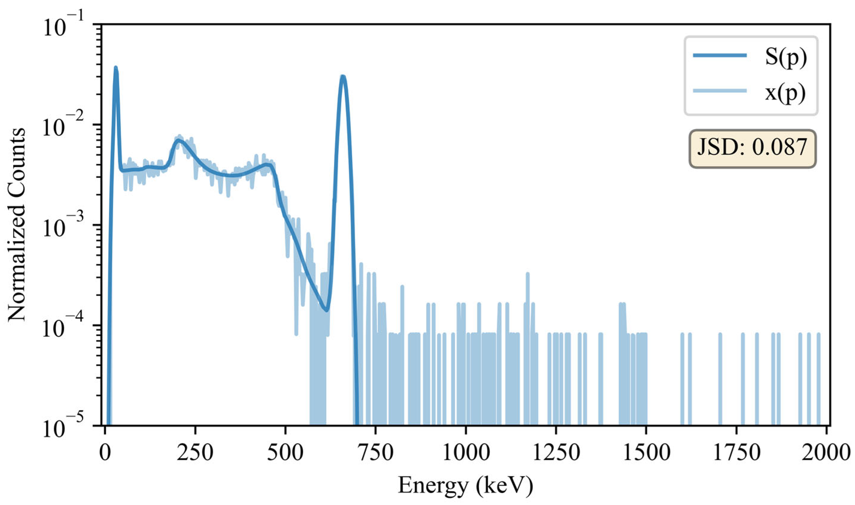
The seeds and samples from the reference configuration were compared to each other. An example of the ¹³⁷Cs seed, $S\left(p\right),$ and one sample, $x\left(p\right),$ can be observed in Figure 2. As a reminder, these single isotope spectra were leveraged for the dissimilarity calculations, but the isotope identification predictions were performed on mixed-isotope spectra. The JSD is leveraged to quantify the similarity between a seed, $S\left(p\right),$ and a corresponding sample, $x\left(p\right)$. It then becomes readily apparent from Figure 2 how there would be a range of JSD values given $N$ samples, $X\left(p\right),$ all with slightly different statistical fluctuations. These seed-to-sample comparisons, $JSD\left(S\right(p\left)\right|\left|X\left(p\right)\right),$ were then carried out for all 26 isotopes and background (BG). The arithmetic means and standard deviations of these baseline comparisons are depicted in Figure 3.

Next, the samples, $X\left(q\right),$ were compared to the seed, $S\left(p\right),$ which then led to the dissimilarity calculations detailed in Equations (2)–(6). In this subsection, there are no domain shifts as $X\left(p\right)$ and $X\left(q\right)$ are both from the same reference configuration. However, all other subsections leverage different configurations for $q$ to quantify the dissimilarity between the training and testing configurations. Figure 4 depicts the results of these comparisons, which, as expected, are very similar. The average JSD values and their uncertainties here will be used as references when evaluating the other configurations detailed in Table 3. As seen in the subsequent sections, the dissimilarity values reported in Figure 4 are relatively low, thus communicating the close resemblance of the two datasets. It should be noted that the background (BG) terms returned higher JSD values due to more significant statistical uncertainty. However, there was still a low dissimilarity value, which was to be expected as both background terms originated from the same configuration.

Figure 5 shows the F1-scores for the four algorithms’ classification performances. Overall, the RF, XGB, and MLP classifiers performed better than the Ridge classifiers. These results serve as reference points, allowing contextualization of the dynamics of the predictive performance when domain shifts are introduced in the testing data. It is important to remind the reader that the data leveraged for the classification task consisted of mixed isotope samples (with statistical noise), as detailed in Section 2.2, while the data used to determine the dissimilarity measures derive from the same measurement configurations, but with only a single isotope, as detailed in Section 2.3.

3.2. Results for Varying Standoff Distance Configurations

Adjusting the standoff distance between a source and a gamma detector has several effects on the corresponding detector response. Increases in standoff distance reduce the total number of recorded counts and increase the spectra’s statistical uncertainty. There may also be more ground scatter with larger distances and fewer pile-up events. All the configurations had minimal dead times <1%; thus, pile-up considerations are negligible. When comparing Figure 6 to Figure 2, the characteristic ¹³⁷Cs 662 keV photopeak is still readily apparent; however, there is a greater degree of statistical noise throughout the spectrum, thus leading to an increased JSD value.

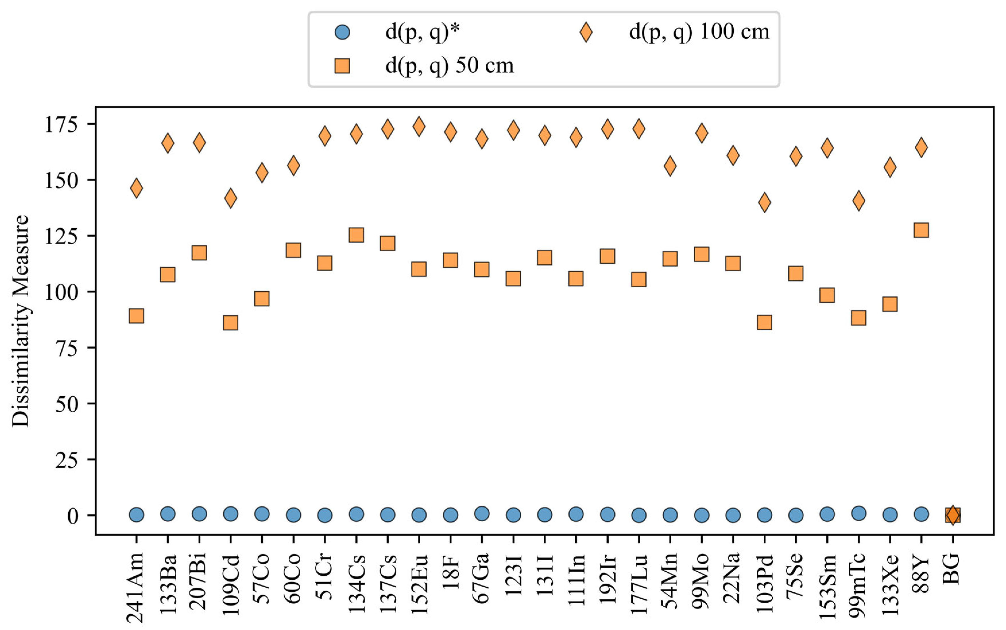
While Figure 6 depicts a single seed-to-sample comparison with a standoff distance of 50 cm, Figure 7 illustrates the dissimilarity between the reference configuration (10 cm standoff) and the 50 cm and 100 cm standoff configurations across all sources examined in this study. There are several key factors to consider when reviewing these dissimilarity results. First, the most significant, or largest dissimilarity is returned with the greatest standoff distance. This result is expected, as this configuration is prone to the greatest statistical uncertainty and, thus, the most significant difference in the spectral shape from the 10 cm reference configuration. Next, the dissimilarity in the BG does not return substantial changes such as those from the other sources. This is not surprising given that changes in the standoff distance do not influence the change in the spectral shape.

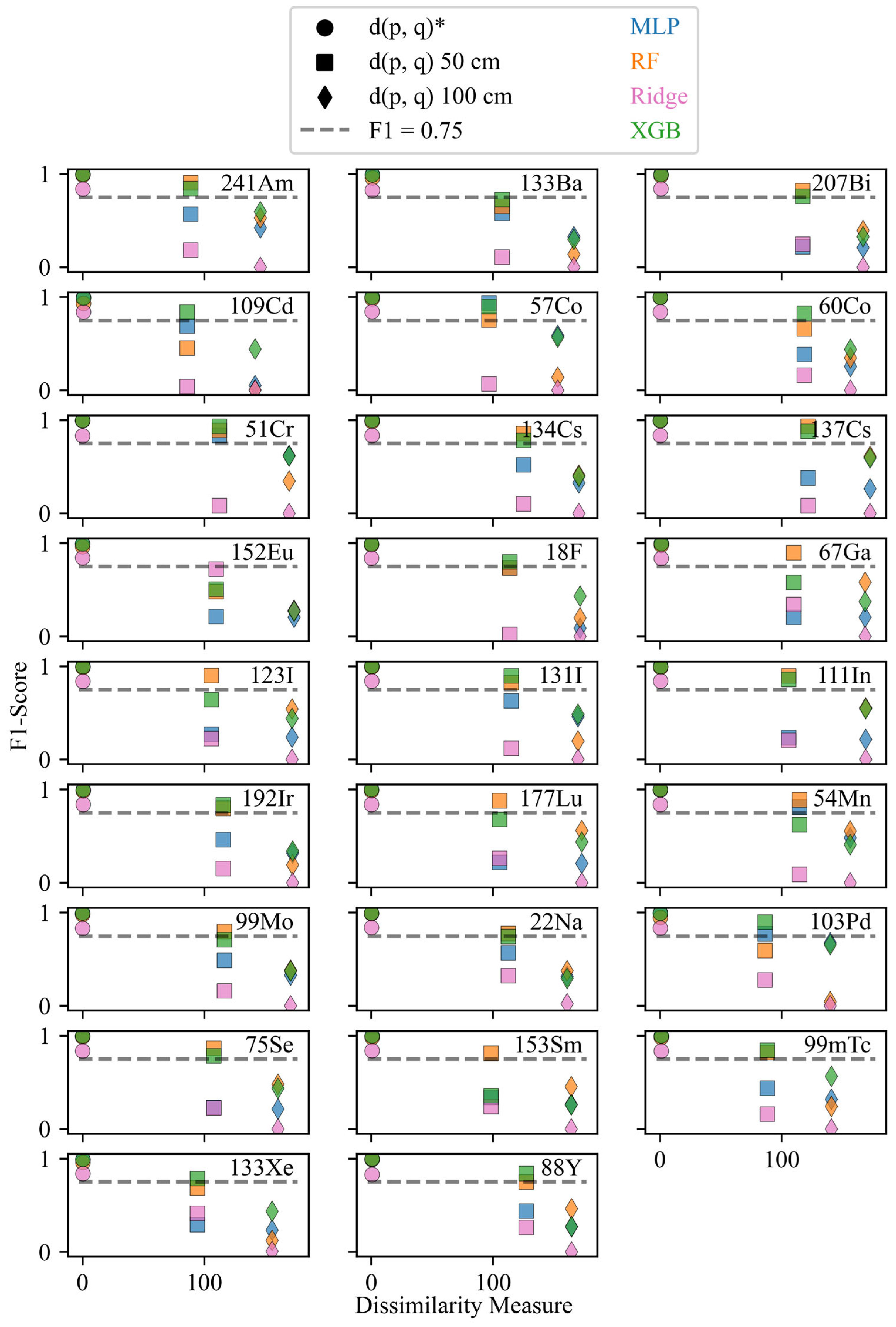
Given that the dissimilarity has been quantified across sources and detection configurations, it is prudent to relate these findings to the classification performance. The F1-scores and the dissimilarity values for the various isotopes are depicted in Figure 8. Horizontal lines are placed in all of the subplots where the F1-score is equal to 0.75, as this provides a quick visual indication of the results. As a general assessment, the predictive performance degraded across the four algorithms as the dissimilarity increased. Examining the predictive performance at the isotopic level reveals interesting results. Over half of the isotopes returned an F1-score over 0.75 for at least one of the four algorithms and a dissimilarity value greater than 100. While no F1-scores above 0.75 were reported for the configuration with a standoff distance of 100 cm, several isotopes were very close, as follows: ⁵¹Cr, ¹³⁷Cs, ¹²³I, ⁵⁴Mn, and ¹⁰³Pd.

To understand the performance comprehensively, the F1-scores of the four algorithms and the dissimilarity values were averaged across isotopes for each configuration and presented in Figure 9. The MLP classifier performed well on the reference configuration and then returned F1-scores that averaged below 0.5 when the standoff distance increased. The Ridge classifier returned the lowest average F1-scores across the configurations. The RF and XGB classifiers performed relatively well, with the only RF classifier returning an average F1-score above 0.75 for the 50 cm configuration.

3.3. Results for Varying Shielding Configurations

One expects variations in the AN and AD of a measurement configuration to influence the underlying spectral shape and statistical uncertainties associated with a spectrum. For instance, the probability of photoelectric absorption increases with the AN and as the energy of the incident photons decreases. Compton scattering events may also occur within a shielding material, thus diminishing the energy of incoming photons and altering the resulting spectral shape. As an example, Figure 10 depicts a seed, $S\left(p\right)$, from the reference configuration $p$, which has no shielding, and a sample from a configuration with iron shielding. Comparing Figure 10 to Figure 2 highlights these changes in the detector response, as the shielding causes a decrease in the magnitude of the ¹³⁷Cs photopeak, the Compton edge and backscatter peak are less defined, the low-energy X-ray peak is squelched, and the overall statistical uncertainty increases. All these variations help drive the increase in the JSD between the seed, $S\left(p\right)$, and the sample, $x\left(q\right)$.

The physics surrounding the interactions of gamma-rays with matter are also evident in Figure 11 when examining the dissimilarity values for the various isotopes. Isotopes such as ¹⁰³Pd and ¹⁰⁹Cd have very low-energy spectral features that are only slightly distorted for the low-Z shielding but return high dissimilarity values when the AN is increased to 20. Conversely, isotopes like ⁸⁸Y and ¹³⁴Cs, which have high-energy spectral features, return lower dissimilarity values due to the shielding, which corroborates with intuition.

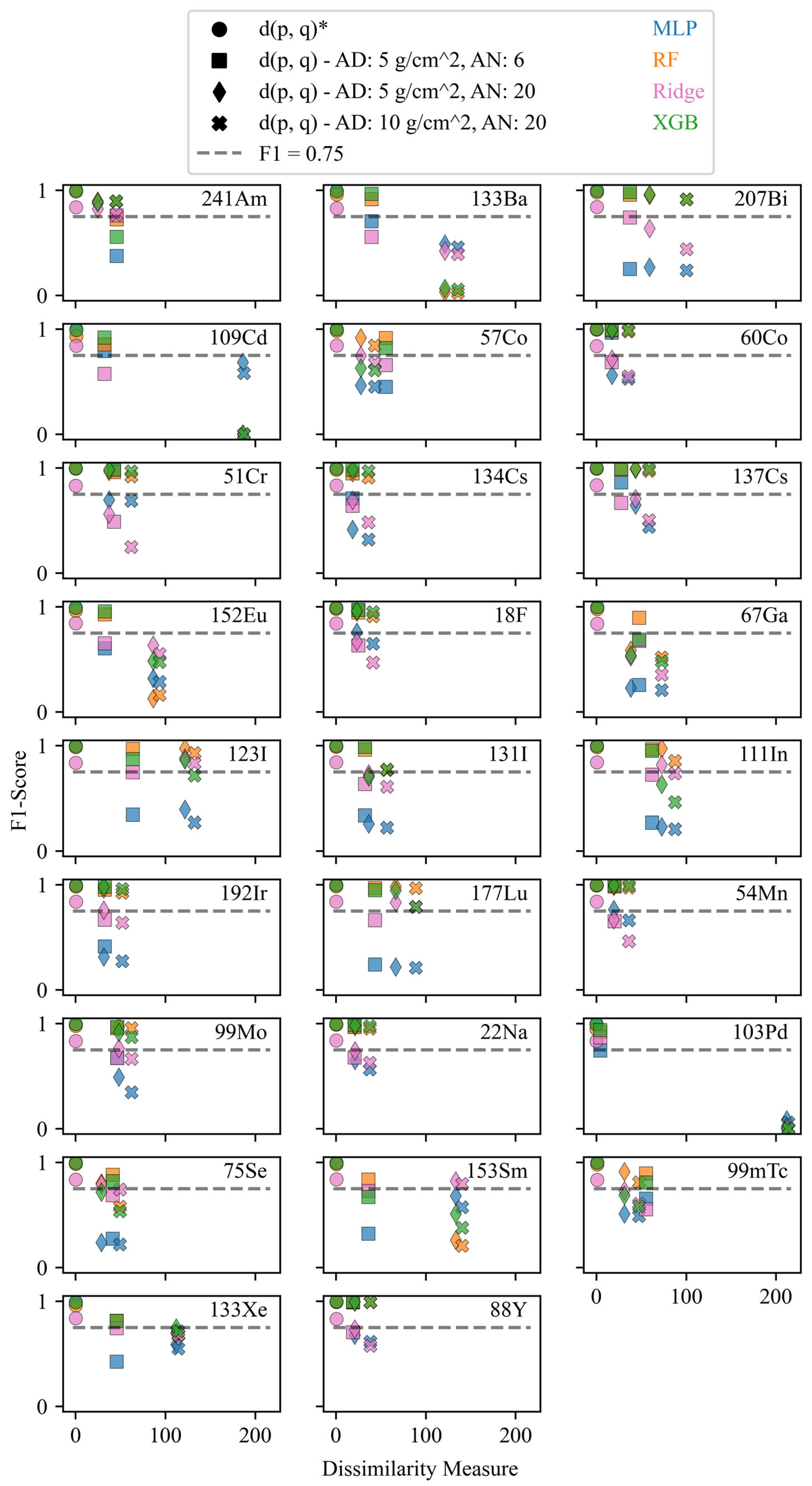
Similar to the results on the varying standoff distances, the F1-scores decreased as the dissimilarity increased. As observed in Figure 12, 18 isotopes returned F1-scores greater than 0.75 for at least one algorithm across all configurations, including ²⁴¹Am, ²⁰⁷Bi, ⁵⁷Co, ⁶⁰Co, ⁵¹Cr, ¹³⁴Cs, ¹³⁷Cs, ¹⁸F, ¹²³I, ¹¹¹In, ¹⁹²Ir, ¹⁷⁷Lu, ⁵⁴Mn, ⁹⁹Mo, ²²Na, ¹⁰³Pd, ^99mTc, and ⁸⁸Y. However, certain isotopes exhibited significant challenges in classification. For instance, ¹³³Ba, ¹⁰⁹Cd, ¹⁵²Eu, and ⁷⁵Se identifications were drastically diminished in the presence of iron shielding. Generally, the RF and XGB classifiers returned higher F1-scores despite the increasing dissimilarity.

While the predominant influence of the increased standoff distance increased the statistical uncertainty, little changed about the underlying spectral shape. With the variations in the shielding configurations, there are changes to the underlying spectral shape and an increase in statistical uncertainties due to the shielding. The F1-scores and dissimilarity values were averaged over all isotopes and reported in Figure 13. This figure shows that the RF and XGB classifiers experience the least degradation in their F1-scores and are the top performers. The MLP classifier, however, returns the lowest F1-scores for the simulated configurations and scores below 0.75 for the measured configurations, suggesting the model’s difficulty generalizing to various shielding scenarios.

3.4. Results for Varying Background Configurations

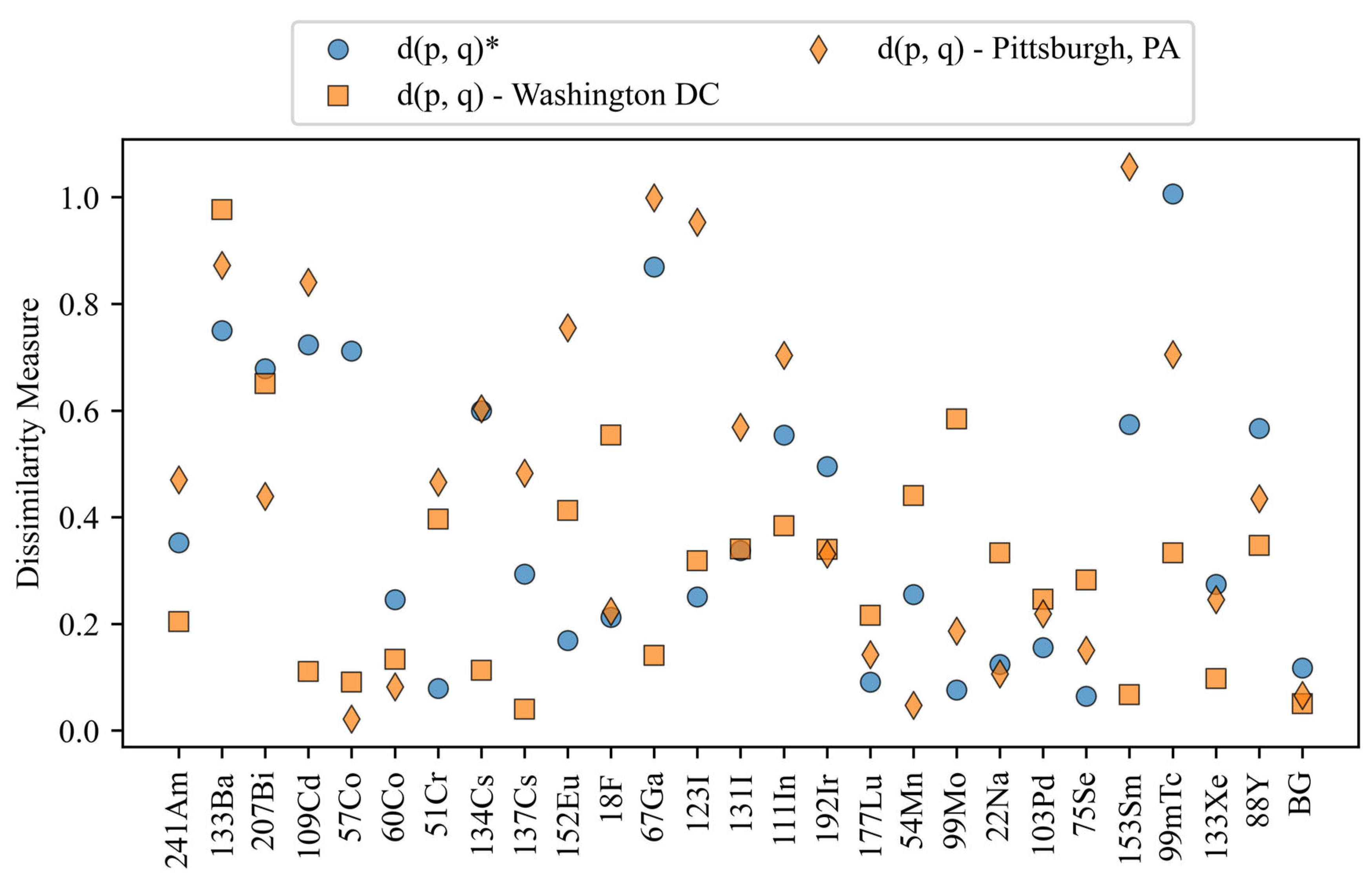
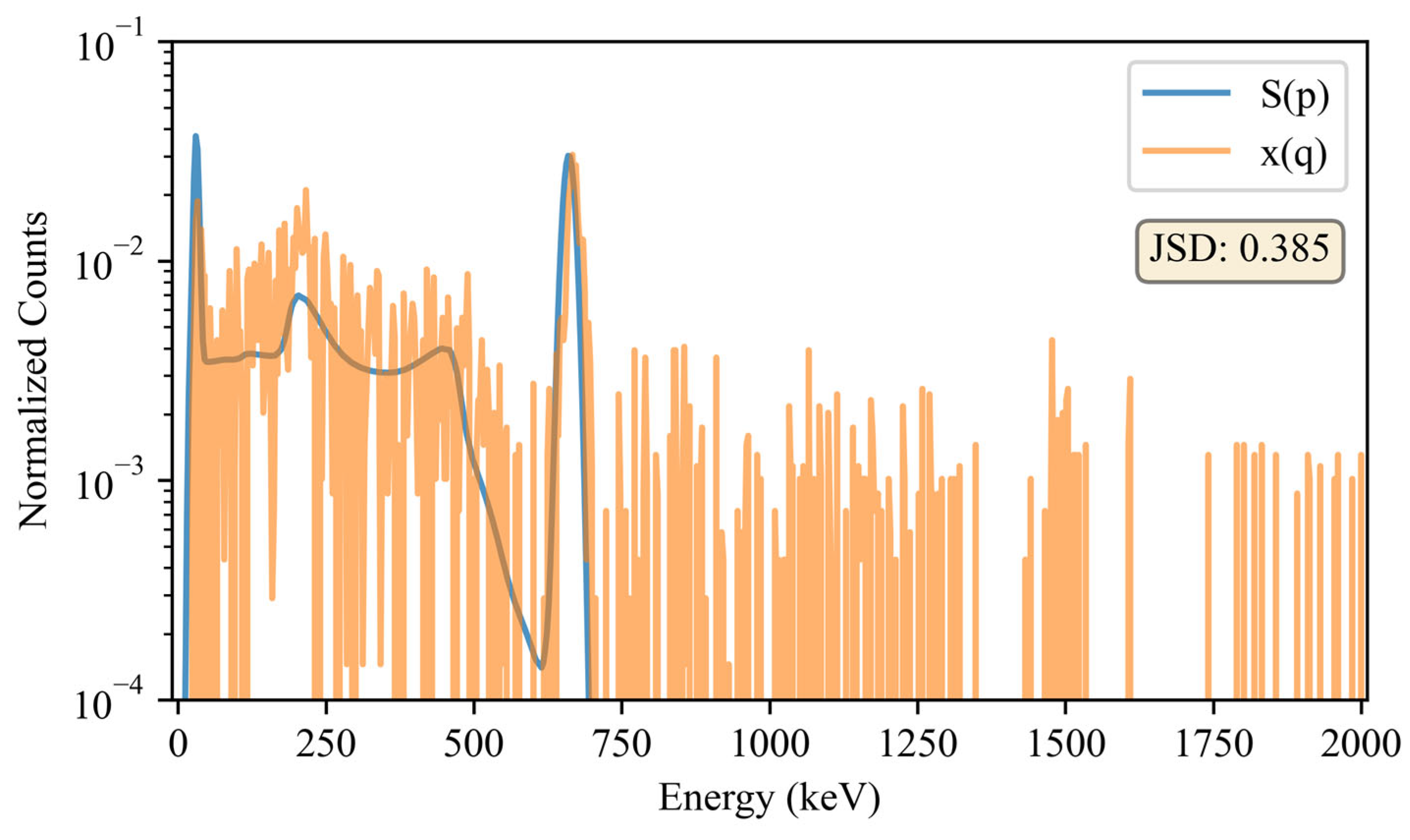
Varying the location of the background measurement can influence the relative proportions of naturally occurring terrestrial and cosmic radioactive constituents in a spectral response. As was described in the methodology, several different geographic locations were leveraged for the testing datasets, resembling Albuquerque, NM; Washington, DC; and Pittsburgh, PA. An example of a background seed, $S\left(p\right)$, from the reference configuration is compared to a background sample, $x\left(q\right),$ resembling Washington, DC, in Figure 14. From this figure, it is challenging to identify discrepancies between the underlying spectral shapes due to the statistical noise of the comparison sample, $x\left(q\right)$.

As observed in Figure 15, there is very little dissimilarity for the synthesized data with the varying background configurations, as there was no change in the spectral shapes of the non-background sources. As mentioned in the analysis of Figure 14, discrepancies exist between the underlying spectral shapes of the backgrounds for the various geographical locations. However, these discrepancies are not prominently manifested due to the statistical fluctuations, thus returning relatively low dissimilarity values.

The lack of relatively large variations in the dissimilarity values for the sources and background leads to relatively consistent predictive performance, as observed in Figure 16 and Figure 17. All of the simulated configurations returned F1-scores above 0.75 across the four algorithms. The MLP and XGB classifiers were consistently the top performers, followed closely by the RF and Ridge classifiers. These results suggest that changes in the background may have less of an influence on ML-based isotope identification than some other measurement parameters, such as shielding and standoff distance.

3.5. Results for Measured Configurations

Domain shifts were incurred by evaluating the ML classifiers on measured data, given that they were trained on synthetic data. Generating simulated spectral data that resembles experimentally acquired data can be very tedious and illusive endeavor. Additionally, there may be nuclear security applications where the time and a priori information necessary to construct such a representative model may not be practical, thus necessitating the employment of an imperfect model. Figure 18 depicts such a scenario where the simulated data represent the reference configuration, and the measured data are also intended to resemble the reference configuration, as there is a 10 cm standoff distance, with no shielding. It should be noted that while the measured configurations closely resemble those being simulated, there are discrepancies between the source activities, thus influencing the overall statistics in the spectra and their resulting comparisons.

While Figure 18 highlights an individual spectral comparison, Figure 19 returns the dissimilarity values determined for the four measured sources (¹³³Ba, ⁶⁰Co, ¹³⁷Cs, ¹⁵²Eu) across the four measured configurations. These values indicate large spectral differences between the training and testing configurations.

Figure 20 and Figure 21 return the F1-scores and dissimilarity values for the four measured sources and their averages, respectively. Because of the differences in the data structures between the measured and synthetic data, robust analysis between Section 3.1, Section 3.2, Section 3.3 and Section 3.4 and this section is inappropriate. However, the same general trends can be observed, such that as the dissimilarity increases, the F1-score decreases. Occasionally, a model will return an excellent performance for a selected isotope in a given configuration (i.e., Ridge classifier, ⁶⁰Co source, and lead-pig configuration) and other times the opposite (i.e., RF classifier, ¹³³Ba source, and concrete configuration). Such spurious results warrant the need to collect and assess more experimental data in future studies.

3.6. Algorithm Performance Comparisons

The previous results assessed the predictive performance of the four algorithms with varying standoff distances, shielding, and backgrounds. These results identified the RF and XGB approaches as consistently returning the best F1-scores across the selected configurations. This discussion summarizes the findings from the previous section by providing a statistical analysis of the prediction results. More specifically, the F1-scores of the various models and configurations were leveraged with Wilcoxon signed-rank tests to assess the statistical significance in the difference in the prediction performances of the models. The Wilcoxon test was selected as it was observed that the differences in the mean F1-scores are non-normally distributed [35]. These findings provide insight into which of the four models is more adaptable to handling domain shifts.

For the Wilcoxon test, the null hypothesis is that there is no difference in the median F1-scores when comparing the two models. To reject the null hypothesis is to say there is a statistical difference in the predictive performance of the models. Values of 0.955, 0.99, and 0.997 were leveraged as confidence intervals in rejecting the null hypothesis.

The results of the Wilcoxon signed-rank tests are partitioned into the following three subsections: Section 3.6.1—analysis of the results from simulated configurations, Section 3.6.2—analysis of the results from both measured and simulated configurations but only for the four measured sources, and Section 3.6.3—analysis of the results for the measured configurations. The discussion was split in this manner to ensure fair and accurate assessments of the results of the models. Each subsection consists of a boxplot and table of the respective F1-scores, followed by the results of the Wilcoxon tests.

3.6.1. Analysis of the Results from Simulated Configurations (All Sources)

Figure 22 and

Table 5. Averaged F1-scores (over 26 sources) for the eight simulated configurations.

Configuration	MLP	RF	Ridge	XGB
Reference configuration	0.995	0.979	0.837	0.995
Standoff: 50 cm	0.477	0.780	0.202	0.763
Standoff: 100 cm	0.312	0.351	0.012	0.434
Shielding—AD: 5 gm/cm2, AN: 6	0.598	0.925	0.670	0.905
Shielding—AD: 5 gm/cm2, AN: 20	0.480	0.752	0.658	0.737
Shielding—AD: 10 gm/cm2, AN: 20	0.423	0.716	0.546	0.693
Background—Washington, DC, USA	0.995	0.979	0.837	0.995
Background—Pittsburgh, PA, USA	0.995	0.979	0.837	0.995

display the average F1-scores across the 26 sources analyzed in this study for the eight simulated configurations. These results show that the Wilcoxon tests were performed as observed in

Table 6. Wilcoxon signed-rank test results from Table 5.

Algorithm1	MLP vs.	MLP vs.	MLP vs.	RF vs.	RF vs.	Ridge vs.
Algorithm2	RF	Ridge	XGB	Ridge	XGB	XGB
Statistic	6.0	9.0	6.0	0.0	17.0	0.0
p-Value	0.109375	0.25	0.109375	0.007813	0.945313	0.007813
Reject null at 95.5% confidence?	No	No	No	Yes	No	Yes
Reject null at 99.0% confidence?	No	No	No	Yes	No	Yes
Reject null at 99.7% confidence?	No	No	No	No	No	No

. In terms of interpreting Table 6 and the label “Algorithm1 vs. Algorthim2”, statistics with a greater magnitude represent significant differences among the median F1-scores. Statistics that are relatively small denote that there is less of a significant difference between the median F1-scores of Algorithm1 and Algorithm2. These results suggest 99.0% confidence that there is a significance difference between the RF vs. Ridge and Ridge vs. XGB results. The other algorithmic comparisons failed to reject the null hypothesis. From a practical perspective, these findings provide statistical evidence that the RF and XGB algorithms implemented in this study are more robust to domain shifts than the Ridge classifier.

3.6.2. Analysis of the Results from Measured and Simulated Configurations (Four Sources)

Figure 23 and

Table 7. Averaged F1-scores for the four measured sources (¹³³Ba, ⁶⁰Co, ¹³⁷Cs, ¹⁵²Eu) for the twelve measured and simulated configurations.

Configuration	MLP	RF	Ridge	XGB
Reference configuration	0.995	0.978	0.836	0.994
Standoff: 50 cm	0.387	0.681	0.267	0.733
Standoff: 100 cm	0.264	0.342	0.070	0.401
Shielding—AD: 5 gm/cm2, AN: 6	0.783	0.952	0.639	0.976
Shielding—AD: 5 gm/cm2, AN: 20	0.503	0.533	0.619	0.634
Shielding—AD: 10 gm/cm2, AN: 20	0.427	0.533	0.499	0.627
Background—Washington DC, USA	0.994	0.978	0.838	0.994
Background—Pittsburgh, PA, USA	0.995	0.979	0.839	0.994
Standoff—10 cm (measured)	0.791	0.962	0.680	0.946
Standoff—50 cm (measured)	0.696	0.554	0.167	0.699
Shielding—Concrete (measured)	0.700	0.590	0.151	0.716
Shielding—Lead pig (measured)	0.669	0.626	0.403	0.666

display the average F1-scores across the measured sources (¹³³Ba, ⁶⁰Co, ¹³⁷Cs, ¹⁵²Eu) analyzed in this study for all twelve configurations. The Wilcoxon tests were performed as observed in

Table 8. Wilcoxon signed-rank test results from Table 7.

Algorithm1	MLP vs.	MLP vs.	MLP vs.	RF vs.	RF vs.	Ridge vs.
Algorithm2	RF	Ridge	XGB	Ridge	XGB	XGB
Statistic	28.0	4.0	10.0	2.0	2.0	0.0
p-Value	0.423828	0.003418	0.020996	0.001465	0.001465	0.000488
Reject null at 95.5% confidence?	No	Yes	Yes	Yes	Yes	Yes
Reject null at 99.0% confidence?	No	Yes	No	Yes	Yes	Yes
Reject null at 99.7% confidence?	No	No	No	Yes	Yes	Yes

. These results indicate that there is 99.7% confidence that there is a significant difference between the RF and Ridge, RF and XGB, and Ridge and XGB results. Additionally, there is 99.0% confidence that there is a significant difference between the MLP and. Ridge results. This statistical analysis reveals that the XGB algorithm significantly outperformed the other algorithms in this study with confidence levels of 95.5% (MLP), 99.7% (RF), and 99.7% (Ridge) across the four measured sources.

3.6.3. Analysis of the Results from Measured Configurations (Four Sources)

Figure 24 and

Table 9. Averaged F1-scores (over the four measured sources (¹³³Ba, ⁶⁰Co, ¹³⁷Cs, ¹⁵²Eu) for the four measured configurations.

Configuration	MLP	RF	Ridge	XGB
Standoff—10 cm (measured)	0.791	0.962	0.680	0.946
Standoff—50 cm (measured)	0.696	0.554	0.167	0.699
Shielding—Concrete (measured)	0.700	0.590	0.151	0.716
Shielding—Lead pig (measured)	0.669	0.626	0.403	0.666

display the average F1-scores across the measured sources (¹³³Ba, ⁶⁰Co, ¹³⁷Cs, ¹⁵²Eu) analyzed in this study for all twelve configurations. The Wilcoxon signed-rank tests were performed as observed in

Table 10. Wilcoxon signed-rank test results from Table 9.

Algorithm1	MLP vs.	MLP vs.	MLP vs.	RF vs.	RF vs.	Ridge vs.
Algorithm2	RF	Ridge	XGB	Ridge	XGB	XGB
Statistic	4.0	0.0	1.0	0.0	1.0	0.0
p-Value	0.875	0.125	0.25	0.125	0.25	0.125
Reject null at 95.5% confidence?	No	No	No	No	No	No
Reject null at 99.0% confidence?	No	No	No	No	No	No
Reject null at 99.7% confidence?	No	No	No	No	No	No

. The Wilcoxon test results reveal that all algorithm comparisons failed to reject the null hypothesis, suggesting the need for the collection of additional measured configurations.

4. Conclusions

Developing accurate and robust ML-based isotope identification capabilities is vital for various nuclear security applications. The accuracy of an ML approach largely depends on how well the training data resemble the testing data. Acquiring training data that closely resemble testing data poses several challenges. For instance, the measurement of interest may be in a scenario or configuration that is restricted or resource-intensive, making it difficult to collect relevant measured data for training. Additionally, synthetic spectral data do not always perfectly match measured configurations, and variations in measurement parameters may exist between the collected data of interest and the parameters used to synthesize the training data due to operational constraints.

While many studies have previously investigated domain adaptation within an isotope identification framework, this study introduces a methodology to quantify the similarity between the training and testing spectra. This technique contextualizes changes in the underlying spectral shape with statistical noise to better communicate the degree of spectral dissimilarity between the training and testing configurations. This dissimilarity was then related to the prediction performances of the four different classifiers to quantify the discussion on algorithm generalizability. Wilcoxon signed-rank tests revealed that the OVR-wrapped MLP, RF, and XGB algorithms generally returned significantly different F1-scores from the Ridge classifier with 95.5% confidence. Additionally, the XGB significantly outperformed the other algorithms with confidence levels of 95.5% (MLP), and 99.7% (RF and Ridge) for the ¹³³Ba, ⁶⁰Co, ¹³⁷Cs, and ¹⁵²Eu sources.

The findings from this work are significant as they outline techniques to promote the development of robust ML-based approaches for isotope identification, a capability vital for various security applications. The novelty of this work is the introduction of a methodology whereby discrepancies between training and testing datasets can be quantified. Additionally, this study evaluates the predictive behavior of several algorithms in the context of the training–testing similarity, which can be beneficial for other developers who may anticipate domain shifts in their spectral analysis. Future studies are anticipated to leverage this work’s methodological developments and results to evaluate the spectral dissimilarity on a greater range of measurement parameters and construct robust analytical and ML tools.

References

1. Mirion Technologies Genie TM 2000. 2017. Available online: https://www.mirion.com/products/technologies/spectroscopy-scientific-analysis/gamma-spectroscopy/gamma-spectroscopy-software/lab-applications/genie-spectroscopy-software-suite (accessed on 15 January 2024).
2. Russ, W.R. Library correlation nuclide identification algorithm. Nucl. Instrum. Methods Phys. Res. Sect. A Accel. Spectrometers Detect. Assoc. Equip. 2007, 579, 288–291. [Google Scholar] [CrossRef]
3. Kamuda, M.; Zhao, J.; Huff, K. A comparison of machine learning methods for automated gamma-ray spectroscopy. Nucl. Instrum. Methods Phys. Res. Sect. A Accel. Spectrometers Detect. Assoc. Equip. 2020, 954, 161385. [Google Scholar] [CrossRef]
4. Kamuda, M.; Sullivan, C.J. An automated isotope identification and quantification algorithm for isotope mixtures in low-resolution gamma-ray spectra. Radiat. Phys. Chem. 2019, 155, 281–286. [Google Scholar] [CrossRef]
5. Kamuda, M.; Stinnett, J.; Sullivan, C.J. Automated Isotope Identification Algorithm Using Artificial Neural Networks. IEEE Trans. Nucl. Sci. 2017, 64, 1858–1864. [Google Scholar] [CrossRef]
6. Koo, B.T.; Lee, H.C.; Bae, K.; Kim, Y.; Jung, J.; Park, C.S.; Kim, H.S.; Min, C.H. Development of a radionuclide identification algorithm based on a convolutional neural network for radiation portal monitoring system. Radiat. Phys. Chem. 2021, 180, 109300. [Google Scholar] [CrossRef]
7. Ghawaly, J.M.; Nicholson, A.D.; Archer, D.E.; Willis, M.J.; Garishvili, I.; Longmire, B.; Rowe, A.J.; Stewart, I.R.; Cook, M.T. Characterization of the Autoencoder Radiation Anomaly Detection (ARAD) model. Eng. Appl. Artif. Intell. 2022, 111, 104761. [Google Scholar] [CrossRef]
8. Wang, Y.; Yao, Q.; Zhang, Q.; Zhang, H.; Lu, Y.; Fan, Q.; Jiang, N.; Yu, W. Explainable radionuclide identification algorithm based on the convolutional neural network and class activation mapping. Nucl. Eng. Technol. 2022, 54, 4684–4692. [Google Scholar] [CrossRef]
9. Fjeldsted, A.; Glodo, J.; Holland, D.; Landon, G.; Scott, C.; Zhu, Y.; Lintereur, A.; Wolfe, D. The Development of a Feature-Driven Analytical Approach for Gamma-Ray Spectral Analysis. Ann. Nucl. Energy 2024, 202, 110464. [Google Scholar] [CrossRef]
10. Zhu, Y.; Fjeldsted, A.; Holland, D.; Landon, G.; Lintereur, A.; Scott, C. Mixture Proportion Estimation Beyond Irreducibility. Proc. Mach. Learn. Res. 2023, 202, 42962–42982. [Google Scholar]
11. Zhu, Y.; Scott, C.D.; Holland, D.E.; Landon, G.V.; Fjeldsted, A.P.; Lintereur, A.T. Fusing Sparsity with Deep Learning for Rotating Scatter Mask Gamma Imaging. In Proceedings of the 2022 IEEE NSS/MIC RTSD—IEEE 2022 IEEE Nuclear Science Symposium and Medical Imaging Conference (NSS/MIC), Milano, Italy, 5–12 November 2022; pp. 1–5. [Google Scholar] [CrossRef]
12. Louis Myers, M.; Charles James, S.; Mayo, M.R. MCNP and GADRAS Comparisons; LA-UR-16-22677; Los Alamos National Laboratory (LANL): Los Alamos, NM, USA, 2016. Available online: https://www.osti.gov/biblio/1248125 (accessed on 15 January 2024).
13. Jeffcoat, R.; Salaymeh, S.; Clare, A. A Comparison of GADRAS-Simulated and Measured Gamma-ray Spectra. In Proceedings of the Institute of Nuclear Materials Management (INMM) Annual Meeting, Aiken, SC, USA, 28 June 2010; pp. 160–185. [Google Scholar] [CrossRef]
14. Ann, K.; Michael, R.; Louis, M. Comparison of Modeled to Measured Spectra Using MCNP and GADRAS to Benchmark and Contrast Modeling Limitations; LA-UR-20-24715; Los Alamos National Lab. (LANL): Los Alamos, NM, USA, 2020. Available online: https://www.osti.gov/biblio/1635509 (accessed on 16 January 2024).
15. Fan, P.; Feng, S.; Zhu, C.; Zhao, C.; Ding, Y.; Shen, Z.; Liu, Y.; Ma, T.; Xia, Y. Radioisotope Identification with Scintillation Detector Based on Artificial Neural Networks Using Simulated Training Data. In Proceedings of the 2020 IEEE Nuclear Science Symposium and Medical Imaging Conference (NSS/MIC), Boston, MA, USA, 31 October–7 November 2020; pp. 1–4. [Google Scholar] [CrossRef]
16. Khatiwada, A.; Klasky, M.; Lombardi, M.; Matheny, J.; Mohan, A. Machine Learning technique for isotopic determination of radioisotopes using HPGe γ-ray spectra. Nucl. Instrum. Methods Phys. Res. Sect. A Accel. Spectrometers Detect. Assoc. Equip. 2023, 1054, 168409. [Google Scholar] [CrossRef]
17. Aage, H.K.; Korsbech, U. Search for lost or orphan radioactive sources based on NaI gamma spectrometry. Appl. Radiat. Isot. 2003, 58, 103–113. [Google Scholar] [CrossRef] [PubMed]
18. Park, J.; Song, G.; Kim, W.; Kim, J.; Hwang, J.; Kim, H.; Cho, G. Identification of radioactive isotopes in decommissioning of nuclear facilities using ensemble learning. Radiat. Phys. Chem. 2024, 220, 111598. [Google Scholar] [CrossRef]
19. Liang, D.; Gong, P.; Tang, X.; Wang, P.; Gao, L.; Wang, Z.; Zhang, R. Rapid nuclide identification algorithm based on convolutional neural network. Ann. Nucl. Energy 2019, 133, 483–490. [Google Scholar] [CrossRef]
20. Moore, E.T.; Turk, J.L.; Ford, W.P.; Hoteling, N.J.; McLean, L.S. Transfer Learning in Automated Gamma Spectral Identification. arXiv 2020, arXiv:2003.10524. [Google Scholar]
21. Chaouai, Z.; Daniel, G.; Martinez, J.; Limousin, O.; Benoit-lévy, A. Application of adversarial learning for identification of radionuclides in gamma-ray spectra. Nucl. Inst. Methods Phys. Res. A 2022, 1033, 166670. [Google Scholar] [CrossRef]
22. Turner, A.N.; Wheldon, C.; Wheldon, T.K.; Gilbert, M.R.; Packer, L.W.; Burns, J.; Freer, M. Convolutional neural networks for challenges in automated nuclide identification. Sensors 2021, 21, 5238. [Google Scholar] [CrossRef]
23. Qi, S.; Wang, S.; Chen, Y.; Zhang, K.; Ai, X.; Li, J.; Fan, H.; Zhao, H. Radionuclide identification method for NaI low-count gamma-ray spectra using artificial neural network. Nucl. Eng. Technol. 2021, 54, 269–274. [Google Scholar] [CrossRef]
24. Ko, K.; Kim, W.; Choi, H.; Cho, G. Feasibility study on a stabilization method based on full spectrum reallocation for spectra having non-identical momentum features. Nucl. Eng. Technol. 2023, 55, 2432–2437. [Google Scholar] [CrossRef]
25. Dinh, T.H.; Cao, V.H.; Dinh, K.C.; Pham, D.K.; Nguyen, X.H. Developing a New Method for Gamma Spectrum Stabilization and The Algorithm for Automatic Peaks Identification for NaI (Tl) Detector. In Proceedings of the Vietnam Conference on Nuclear Science and Technology (VINANST-13), Ha Long City, Vietnam, 6–8 August 2019; pp. 1–10. [Google Scholar]
26. Mitra, P.; Roy, A.S.; Verma, A.K.; Pant, A.D.; Prakasha, M.S.; Anilkumar, S.; Kumar, A.V. Application of spectrum shifting methodology to restore NaI (Tl)-recorded gamma spectra, shifted due to temperature variations in the environment. Appl. Radiat. Isot. 2016, 107, 133–137. [Google Scholar] [CrossRef]
27. Zhang, M.L.; Li, Y.K.; Liu, X.Y.; Geng, X. Binary relevance for multi-label learning: An overview. Front. Comput. Sci. 2018, 12, 191–202. [Google Scholar] [CrossRef]
28. Gamma Detector Response and Analysis Software—Detector Response Function; Version 00; Sandia National Laboratories (SNL): Albuquerque, NM, USA; Livermore, CA, USA, 2014. Available online: https://www.osti.gov/biblio/1231997 (accessed on 16 January 2024).
29. Morrow, T.; Price, N.; McGuire, T. PyRIID; Version 2.0.0; Sandia National Lab (SNL-NM): Albuquerque, NM, USA, 2021. [Google Scholar] [CrossRef]
30. Van Omen, A.; Morrow, T. Controlling Radioisotope Proportions when Randomly Sampling from Dirichlet Distributions in PyRIID; Sandia National Laboratories (SNL): Albuquerque, NM, USA; Livermore, CA, USA, 2024. [Google Scholar] [CrossRef]
31. Romo, J.-R.; Nelson, K.T.; Monterial, M.; Nelson, K.E.; Labov, S.E.; Hecht, A. Classifier Comparison for Radionuclide Identification from Gamma-ray Spectra. In Proceedings of the INMM & ESARDA Joint Annual Meeting, Vienna, Austria, 21–26 August 2021; pp. 1–9. [Google Scholar]
32. Pedregosa, F.; Varoquax, G.; Gramfort, A.; Michel, V.; Thirion, B. Scikit-learn: Machine Learning in Python. J. Mach. Learn. Res. 2011, 12, 2825–2830. [Google Scholar]
33. Chen, T.; Guestrin, C. XGBoost: A Scalable Tree Boosting System. In Proceedings of the 22nd ACM SIGKDD International Conference on Knowledge Discovery and Data Mining, San Francisco, CA, USA, 13–17 August 2016; ISBN 978-1-4503-4232-2. [Google Scholar]
34. Fjeldsted, A.; Morrow, T.J.; Scott, C.; Zhu, Y.; Holland, D.E.; Hanks, E.M.; Wolfe, D. A Novel Methodology for Gamma-Ray Spectra Dataset Procurement over Varying Standoff Distances and Source Activities. Nucl. Inst. Methods Phys. Res. A 2024, 1067, 169681. [Google Scholar] [CrossRef]
35. McDonald, John, H. Handbook of Biomedical Statistics; Sparky House Publishing: Baltimore, MD, USA, 2014. [Google Scholar]
Figure 1. (Left) General schematic of simulated configurations. (Right) Measurement configuration with three sources and 10 cm of concrete between the sources and the detector.
Jne 05 00024 g001
Figure 2. Visual comparison of the seed, S ( p ) , and sample, x p , for a 137Cs source. This is one of the 10,000 baseline comparisons for 137Cs. It should be noted that counts from x ( p ) in the 662 keV photopeak are comparable to that of the seed, S p , thus making it difficult to visualize the sample in this region. Also, counts with energies above the 137Cs photopeak may be attributed to pile-up and statistical uncertainties inherent in background subtraction, which was only employed for the dissimilarity calculations.
Jne 05 00024 g002
Figure 3. Baseline comparisons between the seeds, S p , and samples, X p , of the reference configuration. The mean line represents Ψ μ , p , p , while the error bars represent Ψ σ , p , p . These values are considered “baselines” as they will contextualize the eventual JSD comparisons between S ( p ) and X ( q ) .
Jne 05 00024 g003
Figure 4. The average and standard deviation values for the seed-to-sample comparisons for both the Ψ p and Ψ q comparisons for each source (top). These comparisons were leveraged to calculate the dissimilarity measures for each isotope (bottom). The asterisk denotes the reference configuration where no domain shifts exist between the training and testing data.
Jne 05 00024 g004
Figure 5. F1-scores for each isotope are color-coded for the four algorithms under evaluation. Predictions were made on the reference configuration where there are no domain shifts. A narrow view of the F1-scores is leveraged in this figure to enhance the interpretability of the overlapping markers. However, most other figures will provide a y-axis range of 0–1.
Jne 05 00024 g005
Figure 6. Visual comparison of the 137Cs seed, S ( p ) , where p is the reference configuration and a 137Cs sample x ( q ) , where q is the configuration with a standoff distance of 50 cm. Counts with energies above the 137Cs photopeak are unlikely to be attributed to pile-up but rather statistical uncertainties inherent in background subtraction, which was only employed for the dissimilarity calculations.
Jne 05 00024 g006
Figure 7. Dissimilarity values for the configurations with varying standoff distances. The blue circles represent the dissimilarity values for the reference configuration, and the orange markers are all of the configurations under comparison.
Jne 05 00024 g007
Figure 8. F1-scores and dissimilarity values for the 26 isotopes under varying standoff configurations. The different marker shapes represent the various configurations for the testing datasets, and the color of the markers denotes the algorithm. The asterisk indicates the reference configuration. A dotted line at F1 = 0.75 was included as a visual reference for the performance.
Jne 05 00024 g008
Figure 9. F1-scores and dissimilarity values averaged over all isotopes for each algorithm and standoff distance configuration. The different marker shapes represent the configurations for the testing datasets, and the marker colors denote the algorithms. The asterisk indicates the reference configuration. A dotted line at F1 = 0.75 was included as a visual reference for the performance.
Jne 05 00024 g009
Figure 10. Visual comparison of the 137Cs seed, S ( p ) , where p is the reference configuration, and a 137Cs sample, x ( q ) , where q is the configuration with shielding (AD: 10 g/cm2, AN: 20). Counts with energies above the 137Cs photopeak are unlikely to be attributed to pile-up but rather statistical uncertainties inherent in background subtraction, which was only employed for the dissimilarity calculations.
Jne 05 00024 g010
Figure 11. Dissimilarity values for the configurations with varying shielding. The blue circles represent the dissimilarity values for the reference configuration, and the orange markers are all of the configurations under comparison. The different markers denote the various configurations.
Jne 05 00024 g011
Figure 12. F1-scores for the 26 isotopes under varying shielding configurations. The different marker shapes represent the various configurations for the testing datasets, and the marker colors denote the algorithms. The asterisk indicates the reference configuration. A dotted line at F1 = 0.75 was included as a visual reference for the performance.
Jne 05 00024 g012
Figure 13. Averaged F1-scores and dissimilarity values of the 26 isotopes under varying shielding configurations. The different marker shapes represent the various configurations for the testing datasets, and the marker colors denote the algorithms. The reference configuration is denoted by the asterisks. A dotted line at F1 = 0.75 was included as a visual reference for the performance.
Jne 05 00024 g013
Figure 14. Visual comparison of the background (BG) seed S ( p ) where p is the reference configuration and a BG sample x ( q ) where q is the configuration with a background resembling Washington, DC, USA.
Jne 05 00024 g014
Figure 15. Dissimilarity values for the configurations with varying backgrounds. The blue circles represent the dissimilarity values for the reference configuration, and the orange markers are all of the configurations under comparison. The different markers denote the different configurations. The asterisk indicates the reference configuration.
Jne 05 00024 g015
Figure 16. F1-scores and dissimilarity values of the 26 isotopes under varying background configurations. The different marker shapes represent the various configurations for the testing datasets, and the marker colors denote the algorithms. The reference configuration is denoted by the asterisk. A dotted line at F1 = 0.75 was included as a visual reference for the performance.
Jne 05 00024 g016
Figure 17. Averaged F1-scores and dissimilarity values averaged over all isotopes for each algorithm and shielding configuration. The different marker shapes represent the different configurations for the testing datasets, and the marker colors denote the algorithms. The reference configuration is denoted by the asterisk. A dotted line at F1 = 0.75 was included as a visual reference for the performance.
Jne 05 00024 g017
Figure 18. Visual comparison of the 137Cs seed, S ( p ) , where p is the reference configuration and a 137Cs sample, x ( q ) , where q is the measured configuration with a standoff distance of 10 cm. Counts with energies above the 137Cs photopeak are unlikely to be attributed to pile-up; rather, statistical uncertainties inherent in background subtraction were only employed for the dissimilarity calculations.
Jne 05 00024 g018
Figure 19. Dissimilarity values for the configurations with measured data. The blue circles represent the dissimilarity values for the reference configuration, and the orange markers are all of the configurations under comparison. The different markers denote the various configurations.
Jne 05 00024 g019
Figure 20. F1-scores and dissimilarity values for the four measured sources and their corresponding configurations. The different marker shapes represent the configurations for the testing datasets, and the marker colors denotes the algorithm. A dotted line at F1 = 0.75 was included as a visual reference for the performance.
Jne 05 00024 g020
Figure 21. Averaged F1-scores and dissimilarity values for the four measured sources and their corresponding configurations. The different marker shapes represent the configurations for the testing datasets, and the marker colors denote the algorithm. A dotted line at F1 = 0.75 was included as a visual reference for the performance.
Jne 05 00024 g021
Figure 22. The markers represent F1-scores averaged over all 26 sources at the eight simulated configurations for their respective algorithms. The box plots depict the mean values (center line), interquartile range (box), and min/max values (whiskers).
Jne 05 00024 g022
Figure 23. The markers represent F1-scores averaged over the four measured sources (133Ba, 60Co, 137Cs, 152Eu) for all twelve configurations for their respective algorithms. The box plots depict the mean values (center line), interquartile range (box), and min/max values (whiskers).
Jne 05 00024 g023
Figure 24. The markers represent F1-scores averaged over the four measured sources (133Ba, 60Co, 137Cs, 152Eu) at the four measured configurations for their respective algorithms. The box plots depict the mean values (center line), interquartile range (box), and min/max values (whiskers).
Jne 05 00024 g024