Article

Neutron Yield Predictions with Artificial Neural Networks: A Predictive Modeling Approach

by
Benedikt Schmitz
1,2,* and
Stefan Scheuren
1
1
Institut für Kernphysik (IKP), Technische Universität Darmstadt, Schlossgartenstr. 9, 64289 Darmstadt, Germany
2
Elektrotechnik und Informationstechnik (EIT), Hochschule Darmstadt, Birkenweg 8, 64295 Darmstadt, Germany
*
Author to whom correspondence should be addressed.
J. Nucl. Eng. 2024, 5(2), 114-127; https://doi.org/10.3390/jne5020009
Submission received: 17 October 2023 / Revised: 21 March 2024 / Accepted: 22 March 2024 / Published: 31 March 2024

Abstract

:
The development of compact neutron sources for applications is extensive and features many approaches. For ion-based approaches, several projects with different parameters exist. This article focuses on ion-based neutron production below the spallation barrier for proton and deuteron beams with arbitrary energy distributions with kinetic energies from 3 M e V to 97 M e V . This model makes it possible to compare different ion-based neutron source concepts against each other quickly. This contribution derives a predictive model using Monte Carlo simulations (an order of 50,000 simulations) and deep neural networks. It is the first time a model of this kind has been developed. With this model, lengthy Monte Carlo simulations, which individually take a long time to complete, can be circumvented. A prediction of neutron spectra then takes some milliseconds, which enables fast optimization and comparison. The models’ shortcomings for low-energy neutrons (< 0.1   M e V ) and the cut-off prediction uncertainty ( ± 3   M e V ) are addressed, and mitigation strategies are proposed.

1. Introduction

Research with neutrons is increasingly limited to a few large-scale facilities due to the successive shutdown of European research reactors (as well as the not-far-off completion of the European Spallation Source ESS, the world’s brightest neutron source). The loss of reactors leads to a decrease in available beam time, as can be seen in Figure 1. Smaller facilities and institutes are developing compact neutron sources to continue their research with neutrons [1,2,3,4].
The loss of reactors causes a decline in the available beam time, as displayed in Figure 1. Compact neutron sources have the potential to establish themselves as a backup to large-scale neutron research facilities, as they can be commissioned more quickly and at smaller institutes. Utilizing these sources can increase the available beamtime and give more flexibility to neutron researchers.
Accelerator-based neutron sources, which we discuss here, are scalable. The miniaturization of accelerators generally means that only lower energies can be achieved compared to larger machines, reducing the neutron yield. This makes a trade-off necessary for conventional accelerators since the accelerator cannot become genuinely compact if high energies should be achieved, which increases the final neutron yield. Nuclear waste is less of an issue for particles with energies below the spallation threshold, leaving compactness as the remaining issue [5] (p. 1008 f). This reinforces the goal of keeping the energy below this threshold and aiming for more compact sources. An additional aspect of the design of a compact neutron source is the neutron energy. Higher neutron energies allow us to penetrate thicker materials and increase the number of applications for this source type, for example, in homeland security applications [6].

1.1. Physical Constraints

Most approaches to compact neutron sources are based on the acceleration of light ions (protons or deuterons) impinging on a low-mass target (e.g., lithium, beryllium [1], tantalum [2]) and have particle energies below the spallation threshold (<100 MeV/u) [5] (p. 1008 f). The projects mentioned in this article are based on projectile energies lower than that threshold [1,2,3,7,8].
A method that ensures comparability among these different projects and which is quick to evaluate is essential for developing, comparing, and improving compact neutron sources. Models and results created by the individual institutions for their systems are not necessarily comparable since different nuclear cross-section libraries and measurement methods are used. We developed a model based on simulations and deep learning to ensure this.
This model further allows the evaluation of compact neutron source concepts with non-mono energetic beams, for example, laser-driven ion acceleration via the Target Normal Sheath Acceleration mechanism (TNSA) [7]. TNSA ejects an exponential energy spectrum, which starkly contrasts the mono-energetic particles created by conventional accelerators.

1.2. Outline

The model presented in this work can be used to quickly evaluate neutron source characteristics such as neutron yield, neutron energy, and angular distribution over a wide range of ion energies for proton and deuteron projectiles for several converter materials. This model was originally devised as part of the thesis by B. Schmitz [9] and is here presented in more detail and with additional validations.
Data-driven modeling needs a large dataset of consistent experimental data distributed over the parameter range of interest. Due to insufficient data in the relevant energy range, Monte Carlo simulations were used as the basis for modeling. The simulation results are used to devise a surrogate model based on artificial neural networks to predict the double differential neutron yield with a fast inference of some microseconds. Bootstrap training was performed on the model to predict the uncertainty (refer to Section 2.4). Our model is then compared to experimentally measured neutron spectra and to the model of Wakabayashi et al. [10] to test its validity.

2. Methods

An overview of the steps to be taken is given in Figure 2. The details of the major steps are listed in the remainder of the section.

2.1. Monte Carlo Simulations

We simulated the neutron yield with Monte Carlo Simulations utilizing the PHITS [11] code in Version 3.28A with the FENDL [12] library in Version 3. The observable is the neutron count, which is determined by measuring the number of neutrons crossing a detector’s surface. We implemented several detectors as rings around the converter to resolve the angular distribution. This is illustrated in Figure 3.
We give the concrete parameters for the angle elements (center of the detector) Θ and its size Δ Θ in Appendix A in Table A1.
The ion beam is modeled as a cylindrical beam, starting at position ( 0 , 0 , 9 ) . Its direction is aligned with ( 0 , 0 , 1 ) and the radius is defined as r 0 = 0.5   c m . Energy and particle type of the incoming particles are subject to variation as indicated by Table 1. The converter is given as a cylinder along the z-axis centered around ( 0 , 0 , 0 ) with a radius r = 2.4   c m . The length of the converter is variable and subject to change in this study. Its range is listed in Table 1.
We ensured the target was long enough to stop the full ion bunch inside the target for each energy.
Low-energy neutron absorption and moderation is an effect that has to be taken into account as well. We dealt with this by allowing converters to become longer than the ion stopping range. This is important for non-mono energetic ion beams such as TNSA. TNSA has an exponential energy distribution: if the high-energy part of the spectrum is fully stopped in a converter, then the low-energy part of the spectrum is stopped earlier, leaving more range for the created neutron to interact with the material. These neutrons have a lower final energy due to the moderation inside the remaining converter. If this is not incorporated, the model would overestimate the neutron yield at higher energies. For the parameters of interest, and throughout this study, we acquired 54,768 simulations. Each is generating energy-resolved neutron spectra for 21 distinct scattering angles.

2.2. Data Preparation

Data pre-processing is necessary to ensure the convergence of our model during training. We organized the data as follows: We labeled the categorical data features according to a binary representation of the values, commonly referred to as one-hot encoding. At the same time, we scaled the continuous data from 0 to 1 to its maximum value.
For the categorical data then follows: Each simulation using Deuterium gets assigned a 1, and each simulation using Hydrogen gets assigned a 0. Five different categorical values can only be represented in binary format if three bits are used. Then we can label the different converter materials as: ‘Li’–‘000’, ‘LiF’–‘001’, ‘Be’–‘010’, ‘Va’–‘011’, ‘Ta’–‘100’.
For the continuous parameters of the input features, namely Source Radius, E kin , Length, and Angle, we applied the mentioned normalization to the range of 0 to 1 by dividing each value by the defined maximum value of the parameter, as given in Table 1.
The observable is also a continuously distributed quantity. Since it varies by several orders of magnitude, four steps must be applied to prepare the data for training and ensure numerical convergence.
  • We first resampled the data: The simulation output data were sampled logarithmically and are, therefore, relatively sparse in the higher energy end of the spectrum. With sparse data in the energy component and a decline in the particle count by several orders of magnitude, the stability of the surrogate in this area is in question. We circumvented this by linearly resampling the full spectrum. To acquire this resampling, we applied a cubic spline interpolation of the Monte Carlo output data. Both sets, the raw data and the resampled data, are merged, effectively doubling the number of data points. This resampling increases stability in the higher energy range while it keeps the spectral shape unchanged.
  • We then rescaled the data using the relations given in Equation (1)
    Y ¯ = log 10 Y Y ^ = Y ¯ / min Y ¯
    where Y ^ is the renormalized and Y is the raw data generated by the simulation.
    These two steps are necessary due to the numerical stability of the training process: not only the spareseness of data is problematic in surrogate training. Points with a (orders of magnitude) lower numerical value do contribute much less to the training process metrics than others. As a result, the training process is volatile, which we mitigated by these rescalings.
    As mentioned previously, the ion input energies are below the spallation threshold, and the unit of the spectral data Y is normalized to the reaction’s source particle. This implies that each data point is between 0 and smaller than 1. After both rescaling steps, the converted output data Y ^ of the simulation is normalized and ranges between 1 and the normalized maximal value.
  • The spectrum also consists of energy information to the count rate. We normalized the resulting neutron’s energy E n by the neutron cut-off energy to get a scale from 0 to 1.
    E n ^ X ^ = E n X / max E n
    This results in the energy information range from 0 to 1 and allow us to use all spectra in the same training procedure. These maximum energy values are used later in a second model to predict the cut-off energy.

2.3. ANN Setup

Discontinuities are not smooth and can only be approximated with an even more extensive dataset. Since the physical spectrum has hard cut-off positions representing a discontinuity in the spectrum, we either needed even more data or used a more sophisticated approach. Therefore, we trained two models. The first predicts the normalized spectrum, while the second predicts the cut-off energy.
The networks are both fully connected feed-forward networks. For the spectrum, the node structure is as follows, where x s is an eight-dimensional input vector: ( x s 200 200 200 200 200 200 200 1 ) . For the cut-off energy of the spectrum, the node structure is as follows, where x c is a seven-dimensional input vector: ( x c 260 180 180 340 180 180 340 340 180 1 ) . More details about these input vectors are given in Appendix B.2. For both networks, the split between training and validation data is 90:10. The data for each epoch is taken from the training data and separated again 90:10 into the actual training data and the corresponding testing data.
Further optimization, such as dropout regularization, might acquire better results, but time constraints did not permit further topology optimization. The selected hyperparameters are given in Appendix B.1.

2.4. ANN Bootstrap

The simulation data have, due to their probabilistic nature, an uncertainty. We incorporated this uncertainty with a bootstrap method [13,14]. The raw data were randomly resampled in the range of uncertainty, which is Gaussian distribution, and calculated by PHITS. Taking the Gaussian distribution, we can resample the yield data N times:
Y res = G μ = Y , σ = σ Y ,
where G is the Normal distribution. Applying the same procedure on each resampled spectrum yields N + 1 different predictions, which deviate around the joined mean. For each set of input parameters, N + 1 predictions are generated. The mean of these predictions is then the predicted value, while the standard deviation of those predictions is then the uncertainty of the prediction.

2.5. Ensuring Generality

Our surrogate F maps the input parameters (converter shape, particle parameters) onto the spectrum (double differential yield). The simulated data are normalized to the incident particle. As a result, the model is also normalized. The model’s output must be multiplied by the corresponding particle count N p to determine the actual yield. We can further split non-monoenergetic ion spectra into mono-energetic slices and superpose the results; each summand depends on each slice’s ion energy E p . Furthermore, since the data are binned, the bin width Δ E p must also be considered.
The formal application F is then given by
d 2 Y d Θ d E n = E p N p E p · F ^ E n , Θ , E p , Δ E p
and with the infinitesimal limit for Δ E p 0 :
= N p E p · F ^ E n , Θ , E p , d E p ,
where Y is the neutron yield, Θ the angle under which the observation is made, E n the energy of the neutron, N p the number of incoming projectiles, E p the energy of the projectile, and F ^ is the unit surrogate model, which is normalized to one projectile particle. ∗ denotes all other mentioned parameters from Table 1. E p is sampled according to the needed precision; we used a bin width of Δ E p = 1   M e V . Setting the model up like this enables us to apply and verify this model on mono-energetic spectra and laser-accelerated ions. This model ensures direct comparability between conventional accelerator-driven ion sources and laser-plasma-driven sources.

3. Results

Each network’s final mean squared error and the normalization factor used during preprocessing are displayed in Table 2.

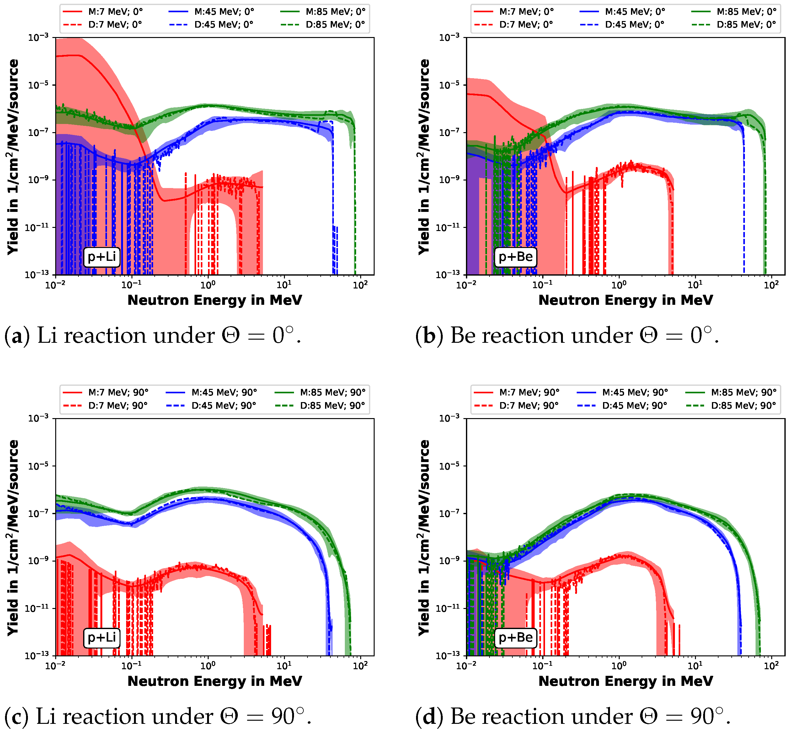
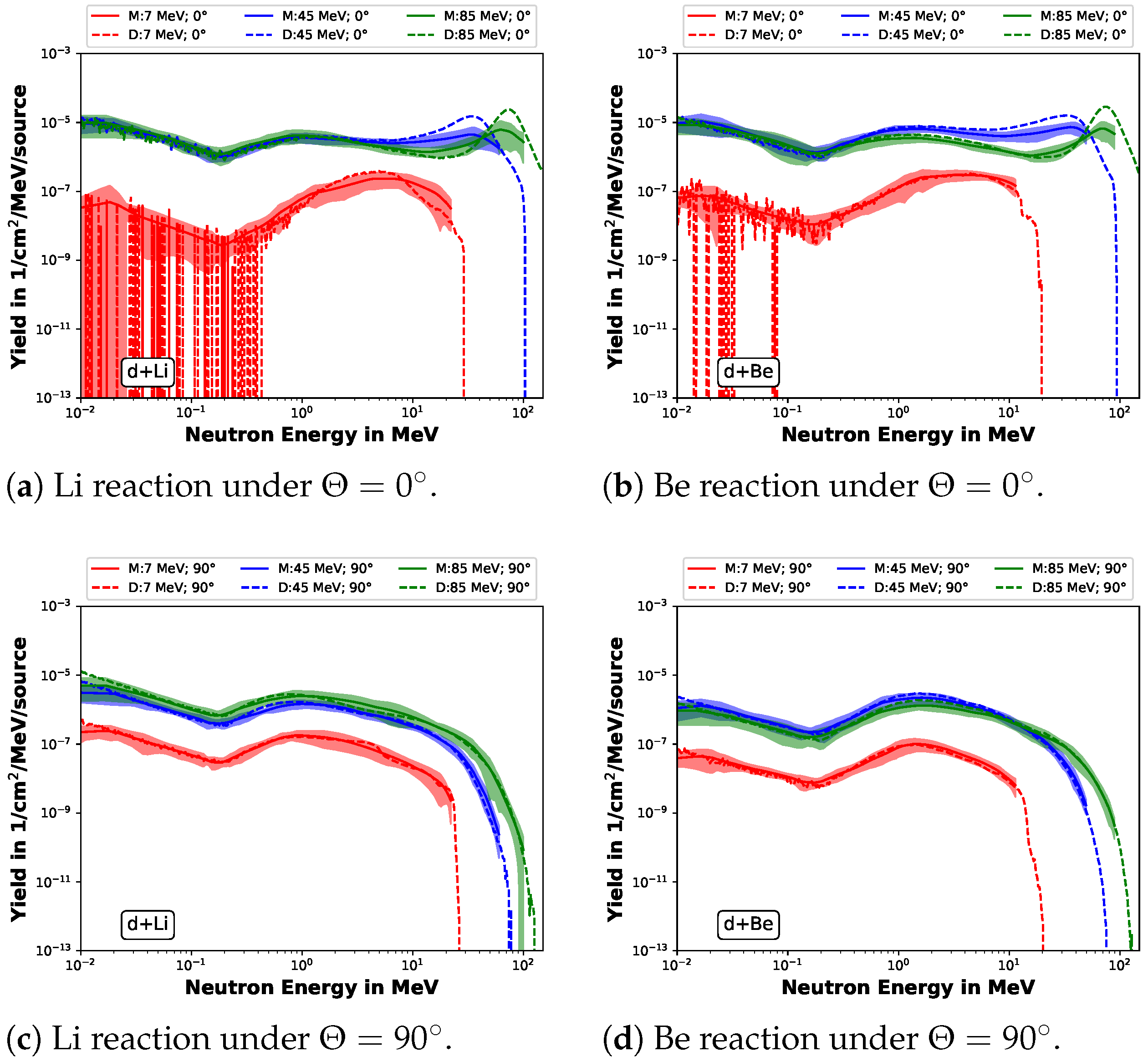
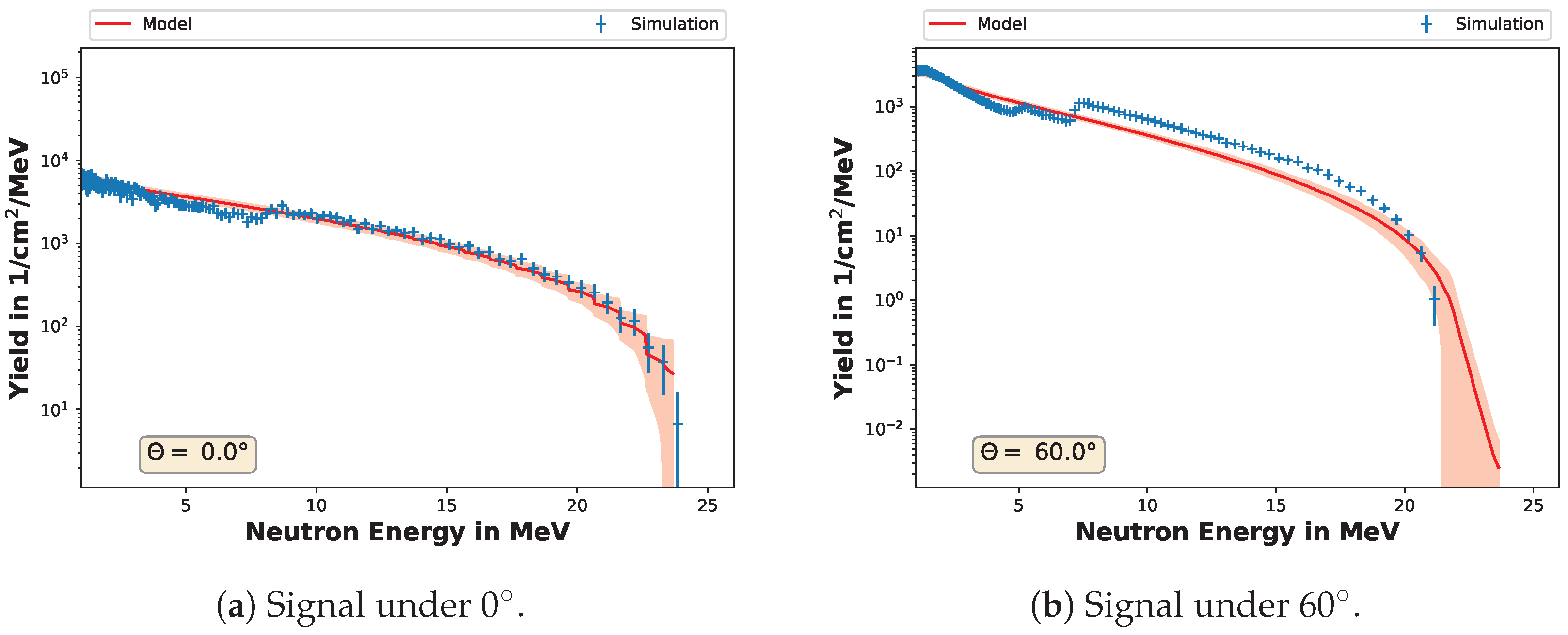
3.1. Validation against the Raw Simulation Data

The validity of the surrogate can be shown by plotting the surrogate’s results with the raw data curves. These curves are displayed in Figure 4 and Figure 5. Displayed are the full spectra created by the Monte Carlo code vs. the result created by our model, with its corresponding uncertainty.
We obtain important constraints of the surrogate regarding its validity from the comparison.
  • The model predictions beyond the parameter range (see Table 1) are not physical.
  • The model can predict the lowest energy neutrons, which cannot be seen in the Monte Carlo spectra. These values, however, have to be used with care: their uncertainty is very high, up to 100%, and the result does not reproduce measurement data correctly (see Section 3.2). The main reason for zero compatible count rates is the bulky target; the lowest neutrons created by low-energy projectiles cannot leave the target and are stuck there or scattered, so they are not counted in the detector. Therefore, the count rates in the simulation are low, meaning the statistical uncertainties are high.
  • The characteristic high-energy peak in the forward direction, which occurs in the p-Li reaction due to the transition from Li-7 to the ground/excited state of Be-7, is suppressed (see Figure 4a). The model is based on regression. Due to this, it further suppresses fast signal peaks. It is, therefore, not capable of resolving these peaks.
  • The cut-off energies mean squared error is approximately 9 M e V 2. This implies an uncertainty of the cut-off energy of approximately ± 3   M e V .
If these limitations are taken into account, we can use the model to predict spectra over a large energy domain in milli seconds of time. How well this model fare against real-world experimental data is discussed and deployed in the following chapter.

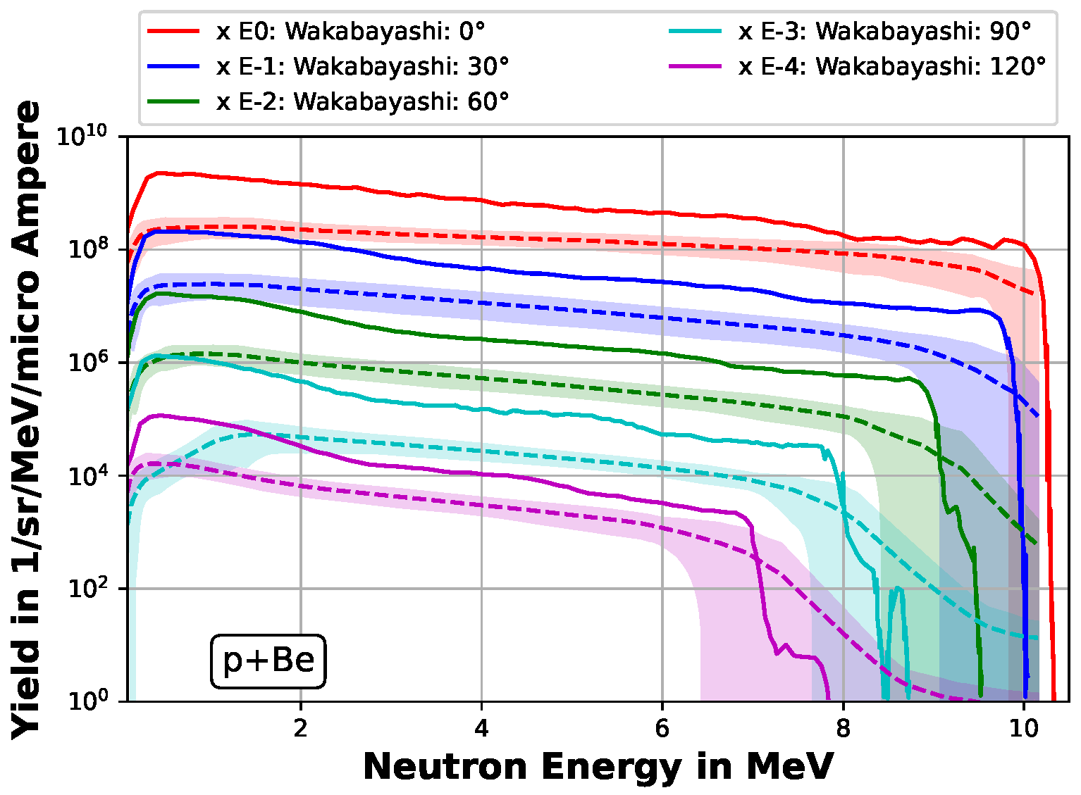
3.2. Validation against Experimental Data

The largest experimental data collection is the EXFOR database, hosted by the International Atomic Energy Agency (IAEA) [15,16]. Only a few datasets are comparable to the model derived here due to different experimental setups, the focus on cross-section measurements with thin targets, and energies of interest larger than 100 M e V . We extracted the corresponding matching data and normalized it to the same units we used in our model.
It is visible that the model, displayed in Figure 6, deviates from the data in the low-energy region below 0.1   M e V . The dataset from Howard et al. taken in 2001 with E p = 3   M e V [17] could not be adequately reproduced and is therefore not displayed here. Both observations have the same reason: For low energy neutrons, the count rates in the Monte Carlo code were too low, and as such, the relative uncertainty is as high as 100%.
The model’s output can also be compared against other modeling approaches. We compare it here with the work from Wakabayashi et al. ([10], Figure 6). The data from the publication are compared with the results of our model in Figure 7.
We normalized our model to the same units as Wakabayashi’s model. The variation between experimental data, JENDL-based results, and the model in the corresponding publication already exceeds up to two orders of magnitude. Our model is continuously lower than the curves from Wakabayashi’s model because our model’s core is based on the JENDL database, resulting in a lower yield. Furthermore, the shape of the converter used in the experimental study is only described as a 2 m m thick Beryllium disc without the radius information. Therefore, our model may further differ from Wakabayashi’s in the converter geometry, increasing the differences between the two models. JENDL was already continuously lower; we can, therefore, conclude that our model behaves indeed as it should. For the forward direction at 0°, we can ensure a good match in the geometry and, therefore, also acquire a spectrum that agrees with the model from Wakabayashi’s work. The larger the observation angle gets, the higher the spectra deviate. Due to the lower experimental yield, we would expect the Beryllium disc to have a radius larger than 24 m m .

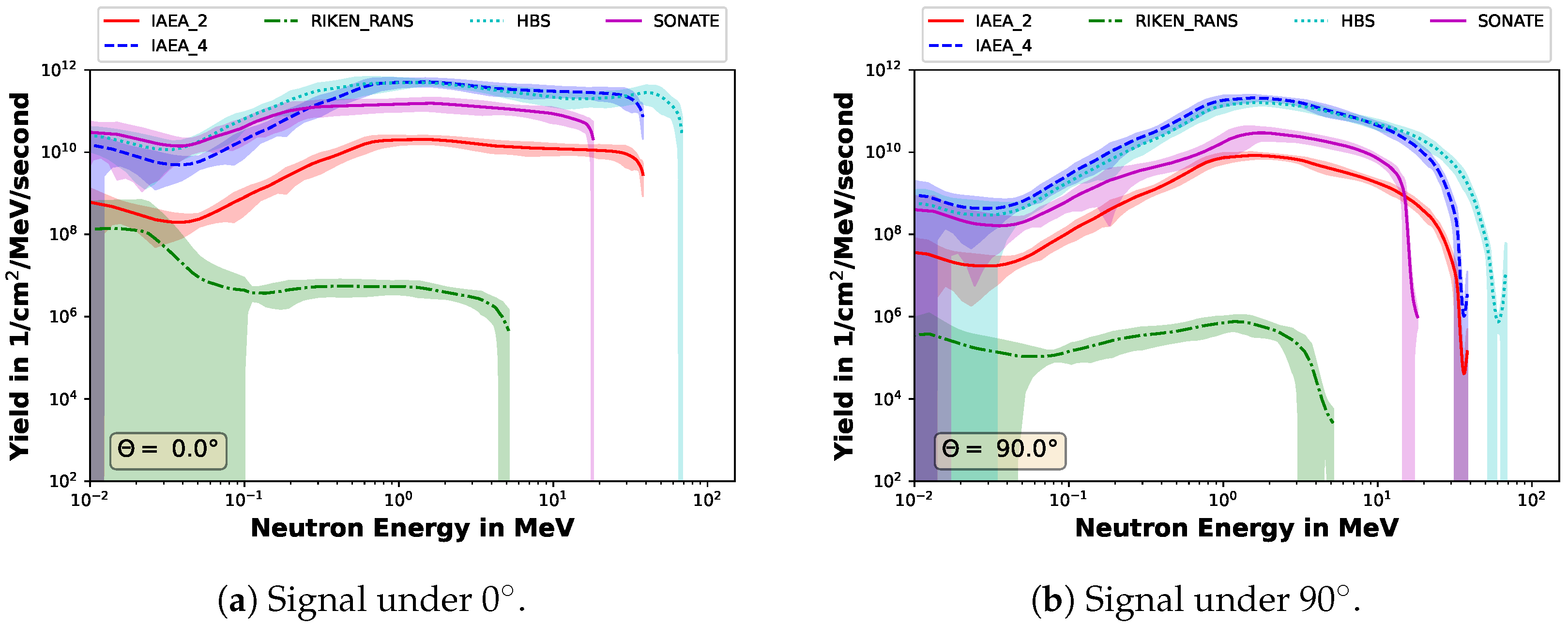
3.3. Spectra for Different Conventional Setups

We can use the model to compare different setups. They vary in the number of particles and the corresponding input energies. Higher ion energy is expected to correlate with a higher neutron yield and higher cut-off energy of the spectrum. The number of neutrons is linearly dependent on the incoming particles due to the superposition principle.
The most progressed concepts and projects for compact neutron sources are based on conventional accelerators. We therefore extracted the relevant parameters from their design reports and used our model to compare those spectra against each other. The projects are the High Brightness Source project (HBS) from Jülich Center for Neutron Science [2], RIKEN accelerator-driven compact neutron systems (RANS) at RIKEN in Japan [1], SONATE at CEA-Saclay [3], and from the technical reports of the IAEA [8]. The parameters used for this evaluation are tabulated in Table 3, and the model’s results are displayed in Figure 8a,b.
Differences in the spectrum result from the different particle energies and the observation angle. The number of incoming ions then scales this spectrum.

3.4. Spectra for Laser-Accelerated Protons

As mentioned previously, the laser-accelerated spectra are calculated by the superposition of several mono-energetic models which follow the composition of the full laser particle spectrum. We tested this on a simulation for the ion spectrum evaluated by Schmitz et al. [20]. The spectrum is analytically given as
d N d E ( E ) = N 0 E exp E k B T ,
where N 0 = 3.7 × 10 11 , k B T = 7.4   M e V , and E the spectrum’s energy in the interval from 5 M e V to 25.5   M e V . We performed additional simulations for this proton spectrum and a corresponding beryllium target with a thickness of 5.02   m m and a radius of 24 m m . The results of the simulations, together with the corresponding model output, are displayed in Figure 9.
The model output is close to the simulation at 0°. At emission angles larger than 60°, the model prediction shows larger deviations from the simulated spectra, indicated by a jump in the spectrum at around 7 M e V . With a larger angle, the neutron’s range inside the converter increases, as the transverse dimension of the target is much larger than the thickness of the target in beam direction (24 m m vs. 5.02   m m ).

4. Conclusions

We presented a predictive surrogate model using an extensive Monte Carlo simulation dataset. This model can be deployed quickly and provides the core for quick evaluations of neutron yields. It increases the accessibility of neutron yield simulations and minimizes the need for experience and training for the complex Monte Carlo tools. Despite insufficient experimental data for data-driven modeling, we showed that our model reproduces experimental datasets if the experimental conditions come close to the model parameters.
Due to our simulation setup and its numerical feasibility, neutrons from projectile energies E p < 5   M e V have a large uncertainty if E n < 0.1   M e V . We recommend not trusting the model in this region without an additional check via a Monte Carlo simulation. The uncertainty, which we calculate by the already explained bootstrapping method in Section 2.4 is a good indicator of the model’s validity.
The next step to improve this model is to investigate the geometry dependency in more detail and to improve the cut-off modeling for the neutron spectra. Both could be achieved by new experimental data or an extension of the simulation model.

Author Contributions

Conceptualization, B.S.; methodology, B.S.; validation, B.S. and S.S.; writing—original draft preparation, B.S. and S.S. All authors have read and agreed to the published version of the manuscript.

Funding

This work was funded by HMWK through the LOEWE center “Nuclear Photonics”. This work is also supported by the Graduate School CE within the Centre for Computational Engineering at Technische Universität Darmstadt. Stefan Scheuren acknowledges support from Trumpf GmbH & Co. KG.

Data Availability Statement

The data used in this study are openly available in tudatalib at https://doi.org/10.48328/tudatalib-1185, reference number 3905. The model and code developed for this study are openly available in tudatalib at https://doi.org/10.48328/tudatalib-1186, reference number 3906.

Acknowledgments

We thank Moritz von Treskow and Dimitrios Loukrezis for the helpful discussions on the data pipeline setup and their thoughts on uncertainty quantification for Artificial Neural Networks.

Conflicts of Interest

The authors have no conflicts of interest to disclose. The funder was not involved in the study design, collection, analysis, interpretation of data, the writing of this article or the decision to submit it for publication.

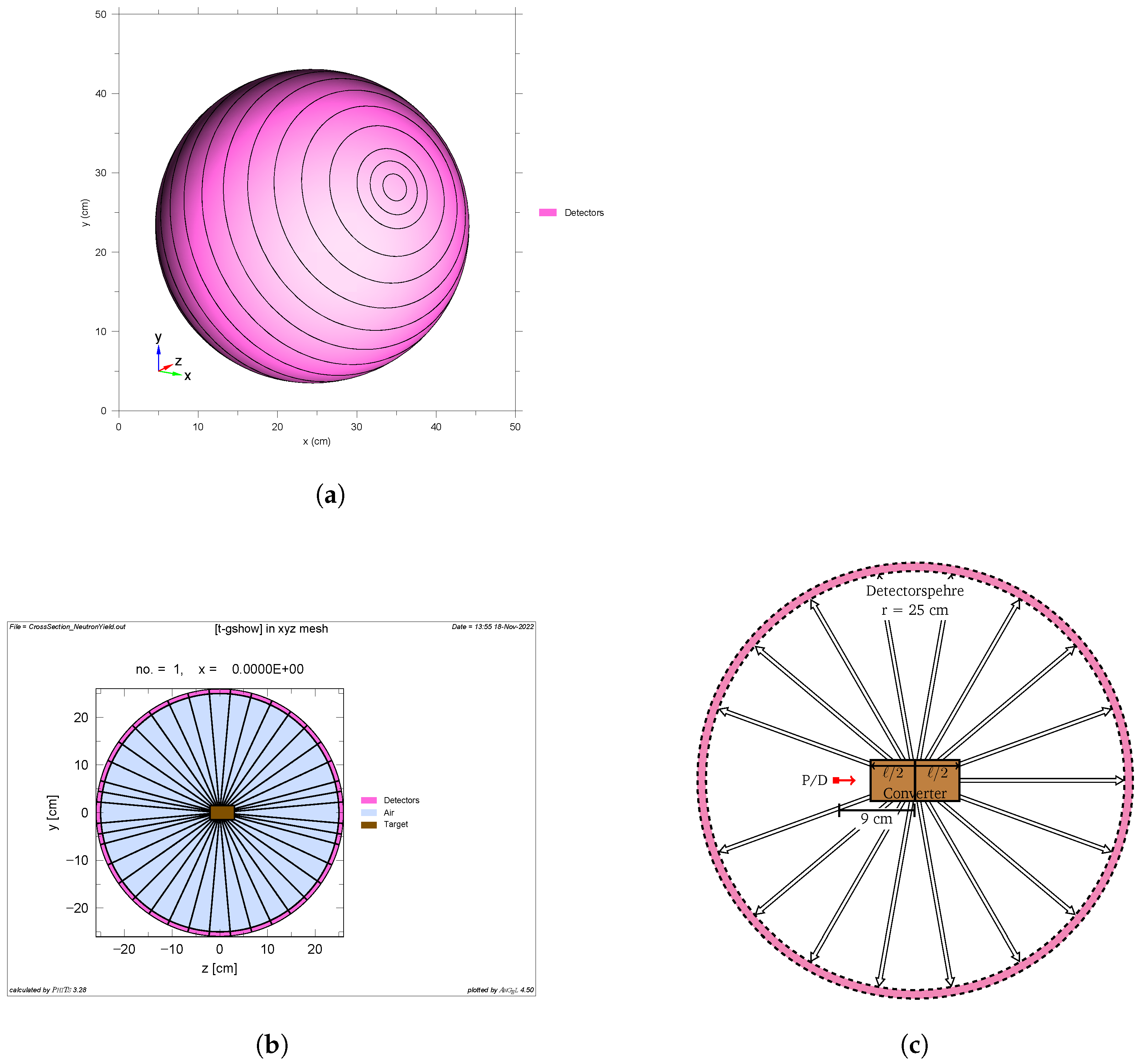
Appendix A. Detector Details

The radius of the detector sphere is 25 c m . The area of the detector is the absolute covered area of the specific detector, and the Ratio is the percentage of full coverage. Θ min and Θ max values describe the minimum and maximum scattering angle the detector can measure. Θ mean is the central scattering angle of the detector.
Table A1. Data for detectors implemented in the Monte Carlo model. Every second value is greyed to guide the eye.
Θ min Θ max Θ mean σ Θ AreaRatio
°°°°cm2%
D01−550.05.014.940.19
D025107.52.544.720.57
D03101512.52.574.150.94
D04152520.05.0234.122.98
D05253530.05.0342.264.36
D06354540.05.0440.005.60
D07455550.05.0524.376.68
D08556560.05.0592.817.55
D09657570.05.0643.248.19
D10758580.05.0674.128.58
D11859590.05.0684.528.72
D1295105100.05.0674.128.58
D13105115110.05.0643.248.19
D14115125120.05.0592.817.55
D15125135130.05.0524.376.68
D16135145140.05.0440.005.60
D17145155150.05.0342.264.36
D18155165160.05.0234.122.98
D19165170167.52.574.150.94
D20170175172.52.544.720.57
D21175185180.05.014.940.19

Appendix B. Parameters and Traits for the Artificial Neural Network Model

Appendix B.1. Hyperparameters

We used the Rectified Linear Unit (ReLU) for the activation function, which is widely used for Regression problems. The identity is employed for the activation function for the last step to the output layer. Similarly, we chose the mean squared error, suited for regression problems, as loss, and it was minimized using the Adam optimizer with β 1 = 0.9 , β 2 = 0.999 and ϵ = 1 × 10 7 . The initial learning rate was 0.001, which was lowered to a minimum of 0.0001 during training should the optimizer detect a plateau in the validation loss value (Keras’ ReduceLROnPlateau feature).
Considering the resampling, each simulation output contains information about ∼500 locations (400 raw data + 100 resampled data) in the energy spectrum. Hence, the available data length for the continuous spectral model was 54,768 × 500 = 2,7384,000 data points. Of these, we used 81% for training, 9% for validation, and 10% for testing. Every training used a batch size of 16 and an early stopping mechanism. Each hidden layer in the network has an L1 regularization strength of 3.56 × 10 7 and an L2 regularization strength of 1 × 10 14 . Since the maximum energy is only predicted per simulation and not per energy bin of the energy spectra, the model for the cut-off energy was trained on 54,768 unique data points. This significantly smaller dataset made the model training faster. The L1 regularization strength was set to 6.2613 × 10 7 , and the L2 regularization strength was set to 2.0392 × 10 8 .

Appendix B.2. Input Vectors

The different input vectors for the two neural networks are constructed as given in Table A2 and Table A3. OHE indicates the one-hot encoding of categorical data. The converter material in the one-hot encoding is represented by three bits.
Table A2. Input vector of the model that predicts the spectrum and its defining quantities.
PositionQuantityOHE/MaxDescription
0 E n [ i ] /150 MeVEnergy value for which the neutron yield should be predicted.
1 E p /100 MeVEnergy of the projectile causing the reaction.
2Length/10.5 cmLength of the converter.
3Theta/180 degreeScattering angle for which the prediction should be done.
4ProjectOHE PThe type of the projectile is encoded with one-hot encoding.
5Conv[0]OHE T1First bit of the one-hot encoded converter material.
6Conv[1]OHE T2Second bit of the one-hot encoded converter material.
7Conv[2]OHE T3Third bit of the one-hot encoded converter material
Table A3. Input vector of the model that predicts the cut-off energy and its defining quantities.
PositionQuantityOHE/MaxDescription
0 E p /100 MeVEnergy of the projectile causing the reaction.
1Length/10.5 cmLength of the converter.
2Theta/180 degreeScattering angle for which the prediction should be done.
3ProjectOHE PThe type of the projectile is encoded with one-hot encoding.
4Conv[0]OHE T1First bit of the one-hot encoded converter material.
5Conv[1]OHE T2Second bit of the one-hot encoded converter material.
6Conv[2]OHE T3Third bit of the one-hot encoded converter material

References

  1. Otake, Y. RIKEN Compact Neutron Systems with Fast and Slow Neutrons. Plasma Fusion Res. 2018, 13, 2401017. [Google Scholar] [CrossRef]
  2. Rücker, U.; Cronert, T.; Voigt, J.; Dabruck, J.P.; Doege, P.E.; Ulrich, J.; Nabbi, R.; Beßler, Y.; Butzek, M.; Büscher, M.; et al. The Jülich high-brilliance neutron source project. Eur. Phys. J. Plus 2016, 131, 19. [Google Scholar] [CrossRef]
  3. Thulliez, L.; Letourneau, A.; Schwindling, J.; Chauvin, N.; Sellami, N.; Ott, F.; Menelle, A.; Annighöfer, B. First steps toward the development of SONATE, a Compact Accelerator driven Neutron Source. EPJ Web Conf. 2020, 239, 17011. [Google Scholar] [CrossRef]
  4. ESFRI Physical Sciences and Engineering Strategy Working Group-NeutronLandscape Group. Neutron Scattering Facilities in Europe—Present Status and Future Perspectives; European Strategy Forum on Research Infrastructures: Brussels, Belgium, 2015; Volume 1. [Google Scholar]
  5. Conrad, H. Handbook of Particle Detection and Imaging; Springer International Publishing: Berlin/Heidelberg, Germany, 2021; Chapter Spallation: Neutrons Beyond Nuclear Fission; pp. 1001–1040. [Google Scholar] [CrossRef]
  6. Buffler, A. Contraband detection with fast neutrons. Radiat. Phys. Chem. 2004, 71, 853–861. [Google Scholar] [CrossRef]
  7. Roth, M.; Schollmeier, M. Ion Acceleration—Target Normal Sheath Acceleration. In CERN Yellow Reports, Volume 1 (2016): Proceedings of the 2014 CAS–CERN Accelerator School: Plasma Wake Acceleration, Geneva, Switzerland, 23–29 November 2014; CAS: Geneva, Switzerland, 2016. [Google Scholar] [CrossRef]
  8. International Atomic Energy Agency. Compact Accelerator Based Neutron Sources; Number 1981 in TECDOC Series; International Atomic Energy Agency: Vienna, Austria, 2021. [Google Scholar]
  9. Schmitz, B. Towards Compact Laser-Driven Neutron Sources: A Numerical Study of Liquid Leaf Targets for High Repetition Rate Laser Experiments and Neutron Production Using Deep Learning. Ph.D. Thesis, Technische Universität Darmstadt, Darmstadt, Germany, 2023. [Google Scholar] [CrossRef]
  10. Wakabayashi, Y.; Taketani, A.; Hashiguchi, T.; Ikeda, Y.; Kobayashi, T.; Wang, S.; Yan, M.; Harada, M.; Ikeda, Y.; Otake, Y. A function to provide neutron spectrum produced from the 9Be + p reaction with protons of energy below 12 MeV. J. Nucl. Sci. Technol. 2018, 55, 859–867. [Google Scholar] [CrossRef]
  11. Sato, T.; Iwamoto, Y.; Hashimoto, S.; Ogawa, T.; Furuta, T.; Abe, S.I.; Kai, T.; Tsai, P.E.; Matsuda, N.; Iwase, H.; et al. Features of Particle and Heavy Ion Transport code System (PHITS) version 3.02. J. Nucl. Sci. Technol. 2018, 55, 684–690. [Google Scholar] [CrossRef]
  12. Forrest, R.; Capote, R.; Otsuka, N.; Kawano, T.; Koning, A.; Kunieda, S.; Sublet, J.C.; Watanabe, Y. FENDL-3 Library Summary Documentation; Technical Report; International Atomic Energy Agency: Vienna, Austria, 2012. [Google Scholar]
  13. Diaconis, P.; Efron, B. Computer-Intensive Methods in Statistics. Sci. Am. 1983, 248, 116–130. [Google Scholar] [CrossRef]
  14. Efron, B.; Stein, C. The Jackknife Estimate of Variance. Ann. Stat. 1981, 9, 586–596. [Google Scholar] [CrossRef]
  15. Otuka, N.; Dupont, E.; Semkova, V.; Pritychenko, B.; Blokhin, A.; Aikawa, M.; Babykina, S.; Bossant, M.; Chen, G.; Dunaeva, S.; et al. Towards a More Complete and Accurate Experimental Nuclear Reaction Data Library (EXFOR): International Collaboration Between Nuclear Reaction Data Centres (NRDC). Nucl. Data Sheets 2014, 120, 272–276. [Google Scholar] [CrossRef]
  16. Zerkin, V.; Pritychenko, B. The experimental nuclear reaction data (EXFOR): Extended computer database and Web retrieval system. Nucl. Instruments Methods Phys. Res. Sect. A Accel. Spectrometers Detect. Assoc. Equip. 2018, 888, 31–43. [Google Scholar] [CrossRef]
  17. Howard, W.B.; Grimes, S.M.; Massey, T.N.; Al-Quraishi, S.I.; Jacobs, D.K.; Brient, C.E.; Yanch, J.C. Measurement of the Thick-Target 9Be(p,n) Neutron Energy Spectra. Nucl. Sci. Eng. 2001, 138, 145. [Google Scholar] [CrossRef]
  18. Kamada, S.; Itoga, T.; Unno, Y.; Takahashi, W.; Oishi, T.; Baba, M. Measurement of energy-angular neutron distribution for 7Li, 9Be(p,xn) reaction at EP = 70 MeV and 11 MeV. J. Korean Phys. Soc. 2011, 59, 1676. [Google Scholar] [CrossRef]
  19. Osipenko, M.; Ripani, M.; Alba, R.; Ricco, G.; Schillaci, M.; Barbagallo, M.; Boccaccio, P.; Celentano, A.; Colonna, N.; Cosentino, L.; et al. Measurement of neutron yield by 62 MeV proton beam on a thick beryllium target. Nucl. Instruments Methods Phys. Res. Sect. A Accel. Spectrometers Detect. Assoc. Equip. 2013, 723, 8–18. [Google Scholar] [CrossRef]
  20. Schmitz, B.; Metternich, M.; Boine-Frankenheim, O. Automated reconstruction of the initial distribution of laser accelerated ion beams from radiochromic film (RCF) stacks. Rev. Sci. Instrum. 2022, 93, 093306. [Google Scholar] [CrossRef] [PubMed]
Figure 1. Different scenarios for the projected availability for neutron beamtime in Europe. Its differences are caused by the assumption of different remaining runtimes from existing machines and different commissions of new instruments, especially at the ESS. Enhanced includes faster commissioning of the ESS instruments and longer runtime, while Degraded assumes faster decommissioning and delays in the ESS commissioning. The detailed explanation for each scenario is given in the ESFRI’s report [4] (pp. 66–77).
Jne 05 00009 g001
Figure 2. Flowchart of the modeling approach and the later usage of the resulting Surrogate model. The dashed lines indicate data flow, the solid lines indicate the input of the parameters from Table 1, and the dashed and dash-dotted lines indicate the surrogate output. The dotted line indicates the spectrum model, and the dash-dotted line indicates the cut-off model. ( X | Y ) are the real Neutron spectra, where X is the energy value and Y ( Y ( X ) ) the count rate at the corresponding X. The hat indicates normalized quantities. The concrete definitions are given in Equations (1) and (2). The predicted quantities are indexed accordingly. Both are needed to extract a physically meaningful spectrum. We would like to reference the supplied scripts and examples for more details. Refer to the data availability statement for further details.
Jne 05 00009 g002
Figure 3. Simulation description plots for the Monte Carlo simulation geometry. (a) CAD of the simulation setup. Created using PHITS Angel tool. (b) Crosssection in the z-y-plane. Created using PHITS Angel tool. (c) Simulation sketch, true to scale, with ion source (red). The converter is centered at the origin.
Jne 05 00009 g003
Figure 4. Model verification against the simulation data for proton-induced reactions. Solid lines indicate the model prediction (M), while the dashed lines are the resulting Monte Carlo spectra (D).
Jne 05 00009 g004
Figure 5. Model verification against the simulation data for deuteron-induced reactions. Solid lines indicate the model prediction (M), while the dashed lines are the resulting Monte Carlo spectra (D).
Jne 05 00009 g005
Figure 6. Experimental data compared to the model (solid lines with shaded uncertainty). (a) Data taken by Kamada et al. in 2011 with E p = 11   M e V [18]. (b,c) contain data taken by Osipenko et al. in 2013 with E p = 62   M e V [19]. The scattering angle is listed in the legend, the model prediction is the same color as the data, and the data have been multiplied by a factor as indicated by the legend’s prefix to increase the readability of the plot.
Jne 05 00009 g006
Figure 7. Our model compared to the data extracted from ([10], Figure 6). Our model gives the dashed lines with the corresponding uncertainty bands.
Jne 05 00009 g007
Figure 8. Model output for the conventional accelerators in p+Be configuration.
Jne 05 00009 g008
Figure 9. Model and simulation output for a TNSA proton beam.
Jne 05 00009 g009
Table 1. Parameters of interest and their range. All parameters needed to set up the Monte Carlo simulations are listed here. Square brackets indicate each continuous interval, while categorical values are comma-separated. Steps indicate the number of possibilities (linearly divided) a parameter can take.
QuantityValuesSteps
ProjectileDeuterons, Protons2
Source Radius/cm0.5fix
E kin /MeV 3 , 97 56
ElementLi, LiF, Be, Va, Ta5
Length/cm 0.002 , 10.445 356
Angle/° 0 , 180 21
Converter Radius/cm2.4fix
Table 2. Network metrics for all trained networks. Id 0 means the raw data are used. The other nine numbers indicate the nine resampled datasets. MSE is the mean squared error training metric, and Normalization indicates the normalization constant applied to each dataset after the logarithm was applied.
IdMSENormalization
00.00128−16.0505
10.00124−16.2796
20.00128−15.9784
30.00119−16.6231
40.00114−16.9578
50.00114−16.8753
60.00125−16.1653
70.00120−16.5274
80.00140−15.3819
90.00121−16.4534
Table 3. Parameters for several conventional compact neutron sources based on ion accelerators. The sources are given in the text.
NameEnergyCurrent d T
UnitMeV10−4 Acm
IAEA240502.0
IAEA44012502.0
RANS710.03
HBS7010001.6
SONATE2010000.2
Disclaimer/Publisher’s Note: The statements, opinions and data contained in all publications are solely those of the individual author(s) and contributor(s) and not of MDPI and/or the editor(s). MDPI and/or the editor(s) disclaim responsibility for any injury to people or property resulting from any ideas, methods, instructions or products referred to in the content.

