A Consistent One-Dimensional Multigroup Diffusion Model for Molten Salt Reactor Neutronics Calculations

Abstract

Molten Salt Reactors (MSRs) have recently gained resurged research and development interest in the advanced reactor community. Several computational tools are being developed to capture the strong neutronics/thermal-hydraulics coupling effect in this special reactor configuration. This paper presents a consistent one-dimensional (1D) multigroup neutron diffusion model for MSR analysis, with the primary aim for fast and accurate calculations for long transients, as well as sensitivity and uncertainty analysis of the reactor. A fictitious radial leakage cross section is introduced in the model to properly account for the radial leakage effects of the reactor. The leakage cross section and other consistent neutronics parameters are generated with the Monte Carlo code Serpent using high-fidelity three-dimensional (3D) models. The accuracy of the 1D consistent model is verified by the reference solution from the Monte Carlo model on the Molten Salt Reactor Experiment (MSRE) configuration. The 1D consistent model successfully reproduced the integrated flux from the 3D model and the reactor multiplication factor k_eff with the error in the range of 95 to 397 pcm (per cent mille), depending on discretized energy group structures. The developed model is also extended to estimate the reactivity loss due to fuel circulation in MSRE. The estimate of reactivity loss in dynamics analysis is in great agreement with the experimental data. This model functions as the first step in the development of a 1D fully neutronics/thermal-hydraulics coupled model for short- and long-term MSRE transient analysis.

1. Introduction

Molten Salt Reactors (MSRs) have recently regained a lot of interest after their inclusion in the Generation IV reactors roadmap [1]. In MSRs, the fuel is dissolved in a molten salt and circulated in the primary loop. This design has several safety and operational advantages, including the elimination of fuel meltdown accidents, online refueling and the continued removal of fission products, high operation temperature and low operation pressure, elimination of fuel fabrication, high negative temperature and void reactivity feedback coefficients [2,3]. On the other hand, the flowing fuel also arises in phenomena that are not present in the current Light Water Reactors (LWRs), such as the drift of the Delayed Neutron Precursors (DNP) with the fuel flow and their redistribution inside the core as a function of the flow speed. Most of the current computational tools for nuclear reactors do not have capabilities to simulate MSRs. This incurs the requirement of developing new tools that have the capabilities to capture the unique characteristics of MSRs to serve in the design and safety analysis of this Generation IV concept.

Many computational tools were developed along the time for the Multiphysics simulation of MSRs. A few of the latest tools in this regard were reviewed in this study. Fiorina et al. [4] developed an axisymmetric two-dimensional (2D), fully coupled Multiphysics model for the MSFR. The models are implemented in COMSOL Multiphysics and TUDelft. The models adopted six and nine energy groups structures for the neutron diffusion equation. Aufiero et. al. [5] used the OpenFoam [6] to develop a three-dimensional (3D), full core, transient model for the MSFR. The model adopted a one-speed neutron diffusion model to reduce the computational cost. Moltres [7], an application for modeling MSRs based on the MOOSE framework [8], used the multigroup diffusion equation in 3D or axisymmetric 2D coupled with the heat equation and the one-dimensional (1D) DNPs drift model. Yang et al. [9] developed a framework for coupling a 3D neutron transport code PROTEUS-NODAL [10] and a modern system-level thermal-hydraulics code SAM [11] to simulate steady-state and transients of MSRs.

All these efforts used either a 3D or an axisymmetric 2D geometry representation of the reactor core, which more-or-less results in high computational cost. The use of such multi-dimensional models is not efficient for long-term transient analysis, neither for the sensitivity analysis or optimization studies. On the other hand, using lower order representation of the geometry, such as a 1D representation, can significantly reduce the computational time and is more suitable for optimization problems and long transients. On the other hand, using such gross 1D models can doubtlessly introduce large errors in the simulation results. However, these errors can be greatly reduced by carefully generating the homogenized material properties, such cross sections. One of the most commonly used methods for generating homogenized cross sections for deterministic diffusion or transport models is based on the Monte Carlo method [12], which includes a detailed simulation of the reactor configuration using a continues energy spectrum to provide a stochastic estimation of the reaction rates. This procedure is followed by collapsing this continues energy spectrum and heterogeneous medium representation into a homogeneous, few-group structure that is suitable for deterministic diffusion codes. The condensation of the cross sections can be generated using infinite spectrum or leakage-corrected spectrum. Serpent [13] has the capability to generate both infinite and leakage-corrected cross sections using the homogenous B₁ method. However, the B₁ method has shortcomings and should be used with caution [14].

In this work, we develop a consistent 1D, multigroup diffusion model for the MSR neutronics analysis, with the primary objective of reducing the computational cost in long transients, sensitivity and uncertainty, and optimization studies of the MSR. Here, the term ‘consistent’ renders our purpose of producing highly agreeable results with the 2D or 3D neutronics models. The consistent diffusion model is achieved with the following measures. The leakage corrected models, counting for both radial and axial leakages, are derived rigorously and integrated into the 1D model. The leakage-corrected parameters are generated using the infinite-spectrum cross sections. Consistent neutronics parameters, including diffusion coefficients and multigroup cross sections, are generated using Monte Carlo 3D models. The procedures of these parameter generation are detailed in the methodology sections.

Another important aim of this work is to develop an accurate and computationally efficient 1D MSR model that can serve for an ongoing US DOE NEUP project—the development of a reactor physics transient benchmark for MSR [15]. This project is being developed based on the legacy data of the Molten Salt Reactor Experiment (MSRE) [16]. The application requires multiple runs for the transient tests conducted during the operation of the MSRE for the purpose of sensitivity analysis. Thus, a 2D or 3D model is not feasible. This paper is organized as follows: the derivation of the 1D consistent model is largely provided in Section 2, the implementation of this model including group parameter generations is discussed in Section 3, and the application of the model for the steady-state and dynamics MSRE analysis are provided in Section 4 and Section 5, respectively, and some concluding remarks on the current model are provided at the end of the paper.

2. Consistent 1D Multigroup Diffusion Model

The time-dependent three-dimensional multigroup diffusion equation may be given by

$$\frac{1}{v_g}\frac{\partial {\varphi }_g}{\partial t}=\nabla ·D_g\nabla {\varphi }_g-{\mathsf{\Sigma }}_{r,g}{\varphi }_g+Q_g,$$

(1)

where $v_g$ is the neutron speed, $D_g$ is the diffusion coefficient, ${\mathsf{\Sigma }}_{r,g}$ is the removal cross section, and $Q_g$ is the neutron source for the gth group, which accounts for the fission source and scattering sources form other groups.

For convenience, we expand Equation (1) in cylindrical coordinates as follows

$$\frac{1}{v_g}\frac{\partial {\varphi }_g}{\partial t}=\left[\frac{1}{r}\frac{\partial }{\partial r}\left(r{D}_g\frac{\partial {\varphi }_g}{\partial r}\right)+\frac{1}{r}\frac{\partial }{\partial \theta }\left(D_g\frac{\partial {\varphi }_g}{\partial \theta }\right)\right]+\frac{\partial }{\partial z}\left(D_g\frac{\partial {\varphi }_g}{\partial z}\right)-{\mathsf{\Sigma }}_{r,g}{\varphi }_g+Q_g,$$

(2)

where the two expanded terms on the right-hand side of the equation represent the planar radial and axial diffusion terms of the diffusion model, respectively.

A one-dimensional model along the axial direction can thus be obtained by integrating Equation (2) over the planner area of the core. By integrating Equation (2) over the planner area A and averaging the resulting quantities over the area, the left-hand side of the equation can be expressed as

$$\frac{1}{A}{\displaystyle \underset{A}{\int }\frac{1}{v_g}\frac{\partial {\varphi }_g(r,\theta ,z,t)}{\partial t}dA=\frac{1}{{\overline{v}}_g}\frac{\partial {\phi }_g(z,t)}{\partial t}},$$

(3)

where ${\phi }_g(z,t)$ is the planner averaged flux

$${\phi }_g(z,t)=\frac{1}{A}{\displaystyle \underset{A}{\int }{\varphi }_g(r,\theta ,z,t)dA},$$

(4)

and ${\overline{v}}_g$ is the flux weighted neutron speed

$$\frac{1}{{\overline{v}}_g}=\frac{{\displaystyle \underset{A}{\int }\frac{{\varphi }_g}{v_g}dA}}{{\displaystyle \underset{A}{\int }{\varphi }_{g}dA}}.$$

(5)

A similar procedure can be performed to define the removal cross sections and other cross sections used to calculate ${\overline{Q}}_g$ (e.g., ${\overline{\mathsf{\Sigma }}}_{f,g}$, ${\overline{\mathsf{\Sigma }}}_{s,g^{\prime }\to g}$). For instance, the area averaged removal cross section is defined as:

$${\overline{\mathsf{\Sigma }}}_{r,g}=\frac{{\displaystyle \underset{A}{\int }{\mathsf{\Sigma }}_{r,g}{\varphi }_{g}dA}}{{\displaystyle \underset{A}{\int }{\varphi }_{g}dA}}.$$

(6)

2.1. Radial Leakage Treatment

The integration form of planner radial diffusion term in Equation (2) can be treated as follows:

$${\displaystyle \underset{A}{\int }\left[\frac{1}{r}\frac{\partial }{\partial r}\left(r{D}_g\frac{\partial {\varphi }_g}{\partial r}\right)+\frac{1}{r}\frac{\partial }{\partial \theta }\left(D_g\frac{\partial {\varphi }_g}{\partial \theta }\right)\right]}rdrd\theta ={\displaystyle \underset{P}{\oint }\left(D_g\frac{\partial {\varphi }_g}{\partial r}\right)}rd\theta +\left(D_g\frac{\partial {\varphi }_g}{\partial \theta }\right)dr,$$

(7)

where the Green’s theorem is applied to convert the area integral to a line integral over the perimeter of the planner area, which equals to the net current leaking in the radial direction

$${\displaystyle \underset{P}{\oint }\left(D_g\frac{\partial {\varphi }_g}{\partial r}\right)}rd\theta +\left(D_g\frac{\partial {\varphi }_g}{\partial \theta }\right)dr=-{\displaystyle \underset{P}{\oint }\left[J_{r,g}rd\theta +J_{\theta ,g}dr\right]}\equiv A{\phi }_g{\mathsf{\Sigma }}_{L,g},$$

(8)

where the radial leakage cross section can be defined as

$${\mathsf{\Sigma }}_{L,g}=\frac{-{\displaystyle \underset{P}{\oint }\left[J_{r,g}rd\theta +J_{\theta ,g}dr\right]}}{A{\phi }_g}=\frac{-{\displaystyle \underset{P}{\oint }\left[J_{r,g}rd\theta +J_{\theta ,g}dr\right]}}{{\displaystyle \underset{A}{\int }{\varphi }_{g}dA}}.$$

(9)

In the case of azimuthal symmetry, $J_{\theta ,g}=0$ and ${\mathsf{\Sigma }}_{L,g}$ is reduced to

$${\mathsf{\Sigma }}_{L,g}=\frac{-2\pi r{J}_{r,g}}{{\displaystyle \underset{A}{\int }{\varphi }_{g}dA}}.$$

(10)

2.2. Axial Leakage Treatment

The axial diffusion term is treated following a similar procedure

$$\frac{\partial }{\partial z}{\displaystyle \underset{A}{\int }{D}_g}\frac{\partial {\varphi }_g}{\partial z}dA=\frac{\partial }{\partial z}{\overline{D}}_g\frac{\partial {\phi }_g}{\partial z},$$

(11)

where ${\overline{D}}_g$ is axial diffusion coefficient, defined as

$${\overline{D}}_g=\frac{{\displaystyle \underset{A}{\int }{D}_g{\varphi }_{g}dA}}{{\displaystyle \underset{A}{\int }{\varphi }_{g}dA}}.$$

(12)

Because the 1D model does not extend to the whole axial domain, appropriate boundary conditions at both ends are needed to account for the axial leakages from two ends of the simulated domain. The response matrix is used to relate incoming current $J_{in,g}$ and the outgoing current $J_{out,g}$ and the boundary surface. For a general G-group energy structure, the relation between partial currents takes the form:

$$\left[\begin{array}{c}{J}_{out,1}\\ J_{out,2}\\ ⋮\\ J_{out,G}\end{array}\right]=\left[\begin{array}{cccc}{\alpha }_{11}& {\alpha }_{21}& \cdots & {\alpha }_{G1}\\ {\alpha }_{12}& \ddots & \cdots & ⋮\\ ⋮& ⋮& \ddots & ⋮\\ {\alpha }_{1G}& \cdots & \cdots & {\alpha }_{GG}\end{array}\right]\left[\begin{array}{c}{J}_{in,1}\\ J_{in,2}\\ ⋮\\ J_{in,G}\end{array}\right].$$

(13)

To implement the albedo boundary condition for the axial directions in the diffusion model, Equation (13) is re-written in terms of the total current and the scaler flux using the definition of the partial currents

$${J_g}^{+}=\frac{1}{4}{\phi }_g-\frac{1}{2}{D}_g\frac{d{\phi }_g}{dz},$$

(14)

$${J_g}^{-}=\frac{1}{4}{\phi }_g+\frac{1}{2}{D}_g\frac{d{\phi }_g}{dz}.$$

(15)

Substituting Equations (14) and (15) into Equation (13) gives

$$\left[\begin{array}{c}\frac{1}{4}{\phi }_1-\frac{1}{2}{D}_1\frac{d{\phi }_1}{dz}\\ \frac{1}{4}{\phi }_2-\frac{1}{2}{D}_2\frac{d{\phi }_2}{dz}\\ ⋮\\ \frac{1}{4}{\phi }_G-\frac{1}{2}{D}_G\frac{d{\phi }_G}{dz}\end{array}\right]=\left[\begin{array}{cccc}{\alpha }_{11}& {\alpha }_{21}& \cdots & {\alpha }_{G1}\\ {\alpha }_{12}& \ddots & & ⋮\\ ⋮& & & \\ {\alpha }_{1G}& \cdots & & {\alpha }_{GG}\end{array}\right]\left[\begin{array}{c}\frac{1}{4}{\phi }_1+\frac{1}{2}{D}_1\frac{d{\phi }_1}{dz}\\ \frac{1}{4}{\phi }_2+\frac{1}{2}{D}_2\frac{d{\phi }_2}{dz}\\ ⋮\\ \frac{1}{4}{\phi }_G+\frac{1}{2}{D}_G\frac{d{\phi }_G}{dz}\end{array}\right].$$

(16)

Equation (16) can be rearranged and written in matrix notations as follows

$$D\frac{d}{dz}\Phi =-\frac{1}{2}{\left(A+I\right)}^{-1}\left(A-I\right)\Phi ,$$

(17)

where $I, A$ are the identity and response matrices, respectively, and $D, \Phi$ are given by

$$D=\left[\begin{array}{cccc}{D}_1& 0& \cdots & 0\\ 0& D_2& & ⋮\\ ⋮& & \ddots & 0\\ 0& \cdots & 0& D_G\end{array}\right],\Phi =\left[\begin{array}{c}{\phi }_1\\ {\phi }_2\\ ⋮\\ {\phi }_G\end{array}\right].$$

(18)

In this work, the albedo coefficients are calculated by tallying the partial currents at the lower and top heads of the reactor vessel, and assuming that all the off-diagonal elements of the response matrix are zero.

2.3. Multigroup Diffusion Equation

With all the factors considered above, the consistent 1D form of Equation (2) can then be written as

$$\frac{1}{{\overline{v}}_g}\frac{\partial {\phi }_g}{\partial t}=\frac{\partial }{\partial z}{\overline{D}}_g\frac{\partial {\phi }_g}{\partial z}-{\stackrel{⌢}{\mathsf{\Sigma }}}_{r,g}{\phi }_g+{\overline{Q}}_g,$$

(19)

where ${\stackrel{⌢}{\mathsf{\Sigma }}}_{r,g}$ is the sum of the group removal and radial leakage cross sections

$${\widehat{\mathsf{\Sigma }}}_{r,g}={\overline{\mathsf{\Sigma }}}_{r,g}+{\mathsf{\Sigma }}_{L,g}.$$

(20)

Note that in the course of the derivation, the group constants were assumed to be a function of the axial position $(z)$. In the case of generating homogenized cross sections for 3D regions, all cross sections should be averaged over the axial dimension too. In this case, the leakage cross section becomes:

$${\mathsf{\Sigma }}_{L,g}=\frac{-{\displaystyle \underset{S}{\iint }{J}_g·d\overrightarrow{S}}}{{\displaystyle \underset{V}{\iiint }{\varphi }_{g}dV}},$$

(21)

where $S$ is the radial surface area of the homogenized region, and $V$ is the volume.

3. Consistent Neutronics Parameters for MSRE

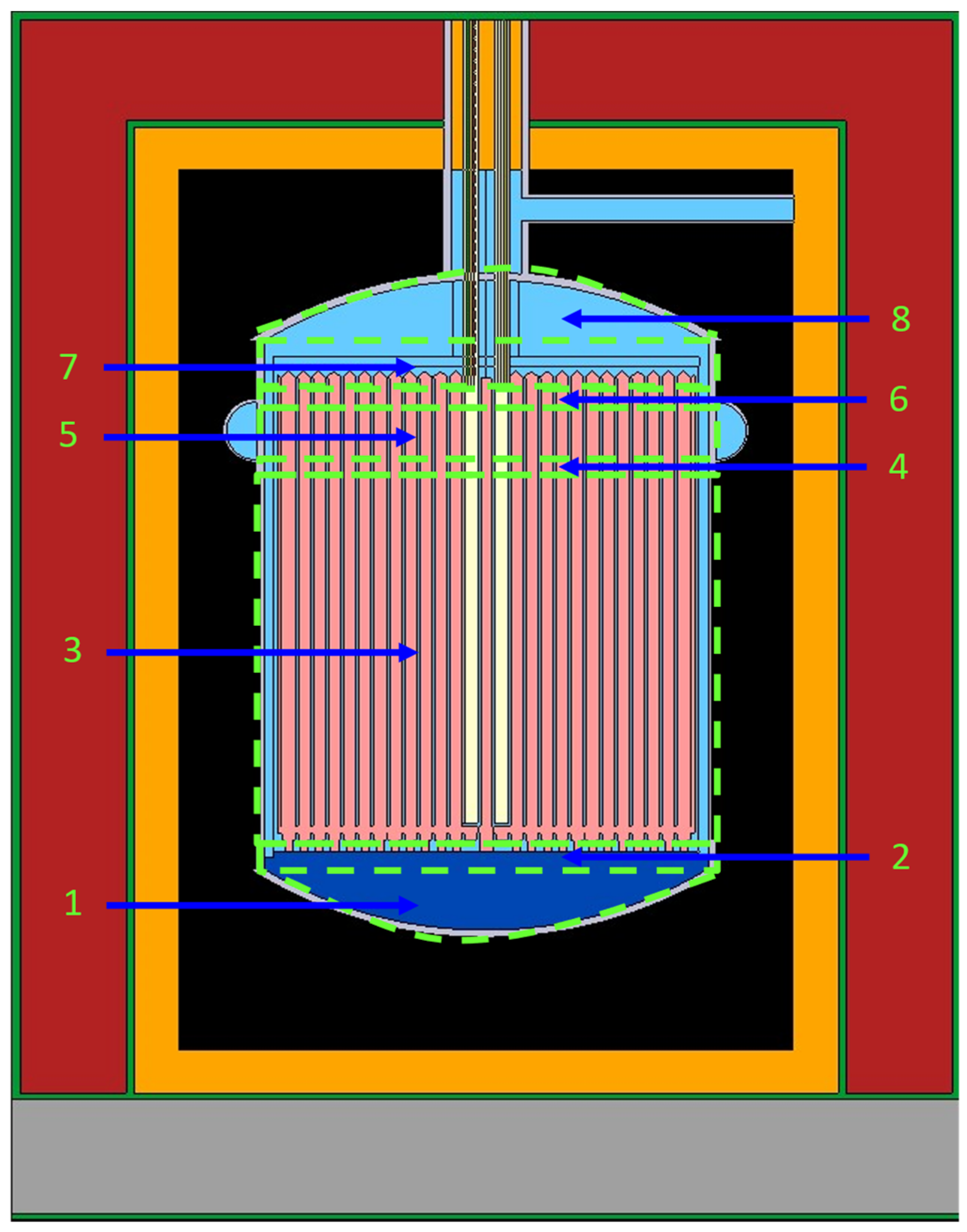
In this section, the numerical implementation of the planar averaged, 1D diffusion model is discussed. The homogenized cross sections and parameters used to calculate the leakage cross sections and the albedo coefficients were generated using the Monte-Carlo transport code Serpent [13]. We followed the MSRE static model provided in Ref. [17], and divided the reactor vessel into eight homogenized regions in the axial direction. The boundaries of each homogeneous region (see Figure 1) were chosen based on the changes in material and/or configuration between the different regions. The homogenized regions, as labelled in Figure 1, include:

(1)

The curved lower head;

(2)

The straight section of lower head;

(3)

The main reactor section;

(4)

The below flow distributor ring;

(5)

The flow distributor ring;

(6)

The above flow distributor ring;

(7)

The straight section of upper head;

(8)

The curved upper head.

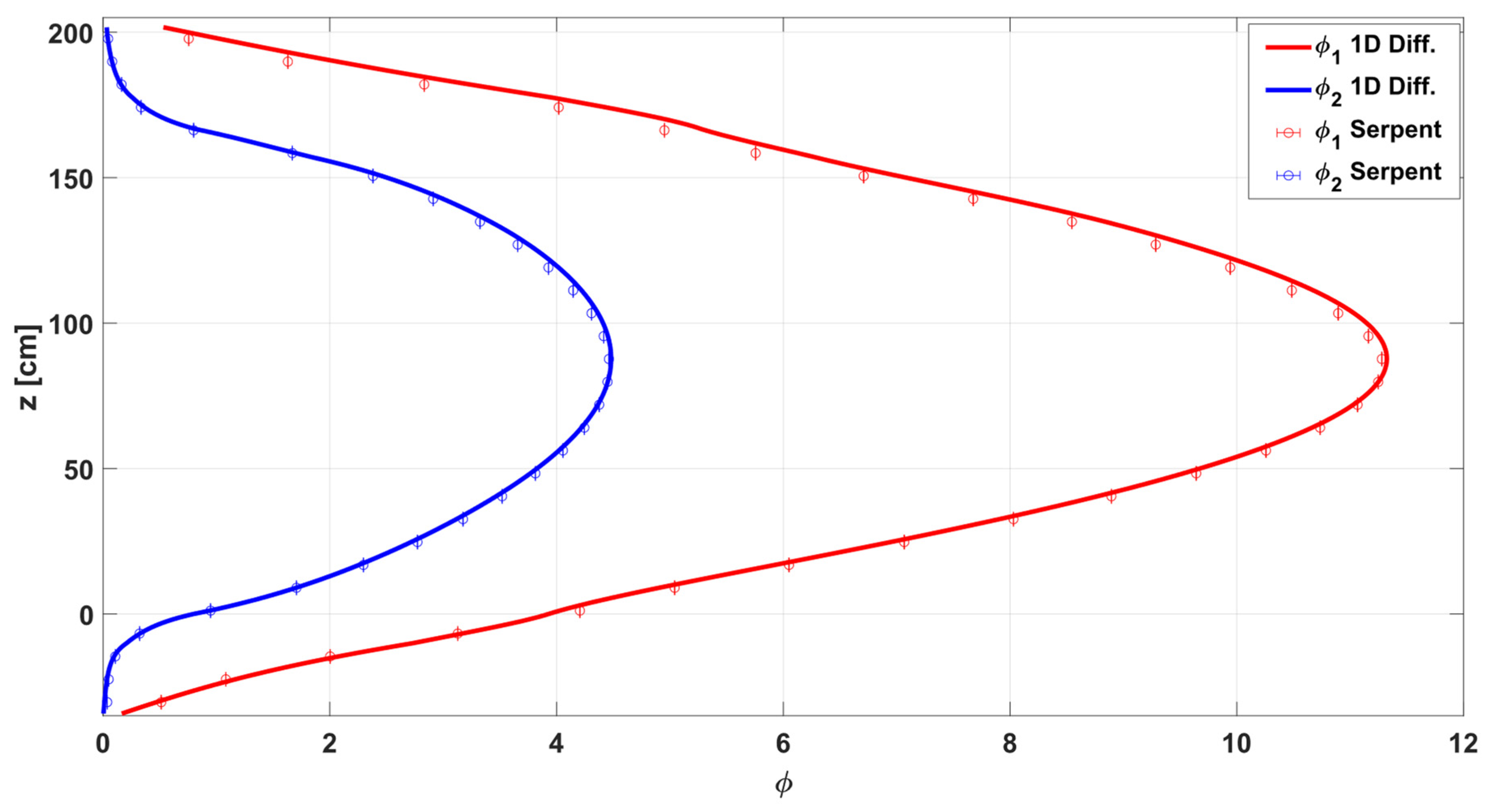
For clarification, the molten salt fuel flowing effect is ignored in the homogeneous parameter generation procedure because the static Serpent model is used as the base reference model at this step. Following the simplification, the viability of the consistent 1D model is firstly verified by the 3D Serpent model steady-state calculation results in Section 4, and then extended for the dynamics analysis in Section 5 with the DNP drift effect taken into account.

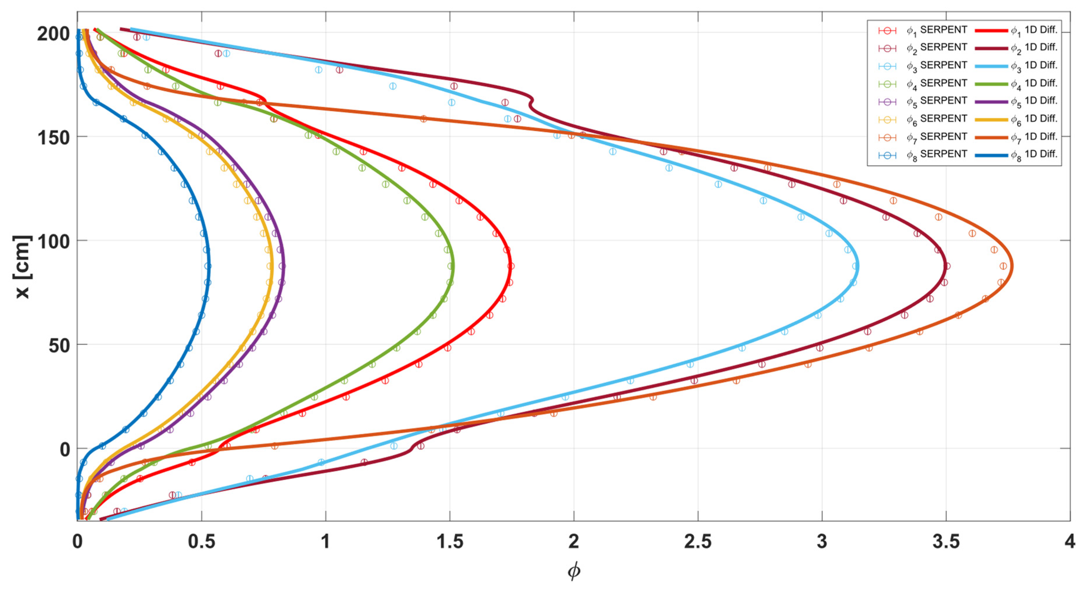
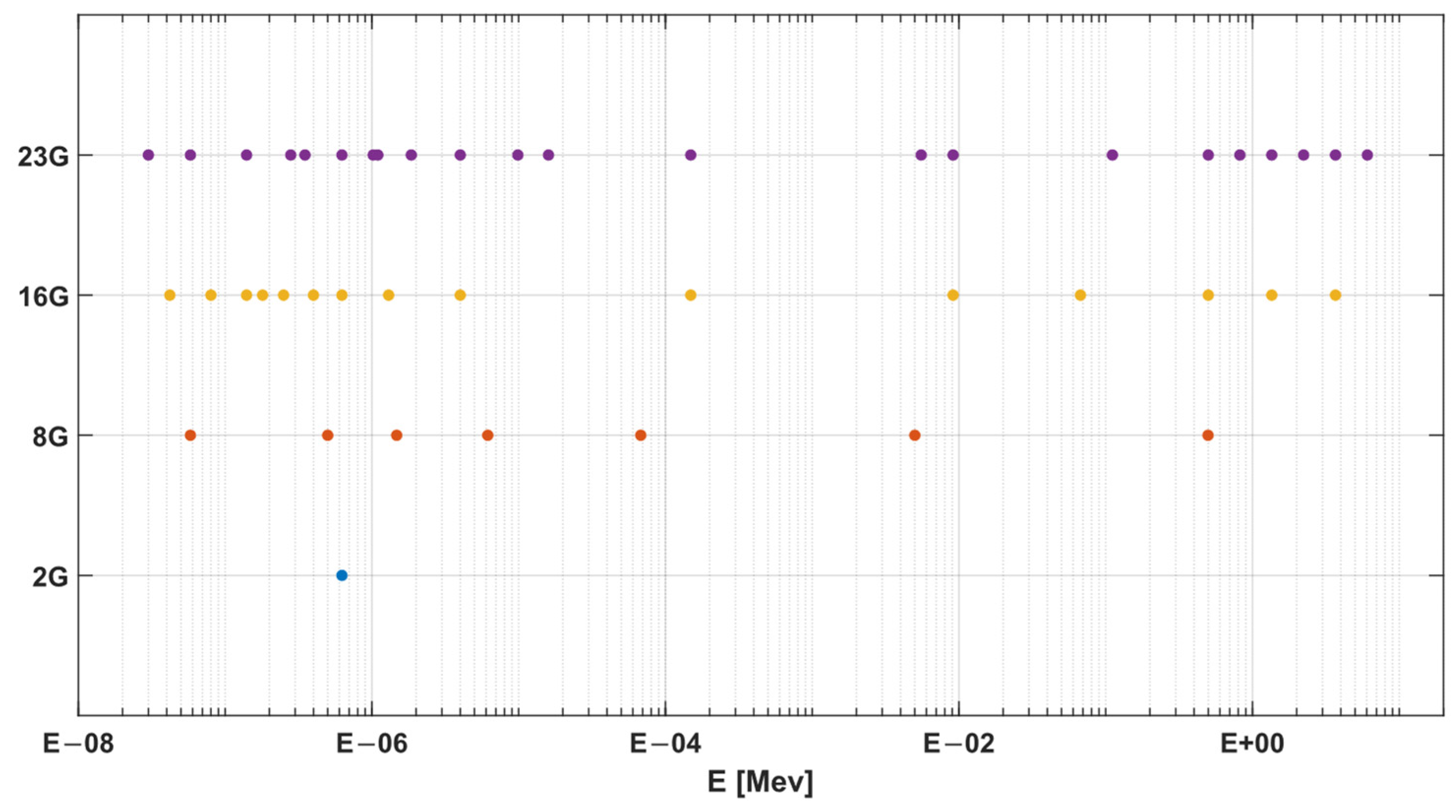
The standard homogenous cross sections were generated in Serpent using the infinite spectrum approach, in which the homogenization is carried out on an infinite lattice of identical cells (i.e., no net current on the cell boundaries) [12]. This approach was chosen because the leakage effect was accounted for in the leakage cross section and the albedo BCs. Four different energy group structures were tested in this work. The first group structure is the standard two-group (2G) structure with a cutoff at 0.625 eV. The second group structure is the eight-group (8G) structure adopted in Ref. [18]. The third structure is the 16-group (16G) structure adopted in Ref. [19]. The fourth energy structure is the standard CASMO23 group (23G) structure [20]. The energy boundaries of the 8G structure are given in

Table 1. G case [18].

Group	Upper Energy Boundary (MeV)
1	1.9640 × 101
2	4.9787 × 10−1
3	5.0045 × 10−3
4	6.7904 × 10−5
5	6.1601 × 10−6
6	1.4750 × 10−6
7	5.0000 × 10−7
8	5.8000 × 10−8

. For illustration, the energy boundaries of the different structures tested in this work are summarized and compared in Figure 2, in which the different colors stand for the group boundary points of different energy group.

For the sake of space, only the 2G parameters were presented in this paper. The condensed data for other energy groups were stored and used for the diffusion model in the same manner. The infinite 2G cross sections are summarized in

Table 2. The region-wise homogenized 2G cross sections generated from Serpent using the infinite spectrum approach.

Regions	${\mathit{D}}_1$	${\mathit{D}}_2$	${\mathsf{\Sigma }}_{\mathit{r},1}$	${\mathsf{\Sigma }}_{\mathit{r},2}$	${\mathsf{\Sigma }}_{\mathit{s},1\to 2}$	${\mathsf{\Sigma }}_{\mathit{s},2\to 1}$	$\mathsf{\nu }{\mathsf{\Sigma }}_{\mathit{f},1}$	$\mathsf{\nu }{\mathsf{\Sigma }}_{\mathit{f},2}$
1	8.73 × 10−1	7.57 × 10−1	5.69 × 10−3	4.35 × 10−2	9.97 × 10−4	6.27 × 10−3	1.95 × 10−3	3.21 × 10−2
2	1.02 × 100	9.27 × 10−1	5.17 × 10−3	2.98 × 10−2	1.55 × 10−3	3.40 × 10−3	2.12 × 10−3	3.62 × 10−2
3	1.00 × 100	8.18 × 10−1	4.88 × 10−3	9.05 × 10−3	3.71 × 10−3	2.45 × 10−3	7.21 × 10−4	1.07 × 10−2
4	9.95 × 10−1	8.16 × 10−1	4.98 × 10−3	9.21 × 10−3	3.72 × 10−3	2.47 × 10−3	7.24 × 10−4	1.08 × 10−2
5	9.85 × 10−1	8.16 × 10−1	5.03 × 10−3	9.29 × 10−3	3.71 × 10−3	2.57 × 10−3	7.37 × 10−4	1.07 × 10−2
6	9.95 × 10−1	8.34 × 10−1	4.47 × 10−3	1.14 × 10−2	2.90 × 10−3	2.97 × 10−3	9.55 × 10−4	1.33 × 10−2
7	1.15 × 100	1.06 × 100	4.34 × 10−3	2.72 × 10−2	1.29 × 10−3	3.45 × 10−3	2.28 × 10−3	3.96 × 10−2
8	1.01 × 100	9.42 × 10−1	4.75 × 10−3	3.32 × 10−2	1.00 × 10−3	5.24 × 10−3	2.18 × 10−3	3.60 × 10−2

.

The values of the albedo coefficients used at the boundaries are listed in

Table 3. The 2G diagonal albedo coefficients generated using Serpent for the lower and upper boundaries of the reactor vessel.

Boundary	${\mathsf{\alpha }}_{11}$	${\mathsf{\alpha }}_{22}$
Lower	4.05 × 10−1	1.42 × 100
Upper	3.59 × 10−1	1.18 × 100

. These values were obtained by tallying the partial currents at the curved surface of the lower and upper heads of the reactor vessel. The values of ${\alpha }_{gg}$ were then calculated from $J_{in,g}/J_{out,g}$.

The homogenized radial leakage cross sections are defined by Equation (21) where the numerator is the net current leaking form the outer surface of the region, and the denominator is the integral flux in the homogenized region. The leakage cross sections for the curved sections of both the lower and upper heads (Region 1 and 8) are set to zero, because the leakage from these regions is considered in the albedo BC. The 2G leakage cross sections for the other six homogenized regions are given in

Table 4. The region-wise, 2G radial leakage cross section calculations.

Regions		Integral Flux	Net Current	${\mathsf{\Sigma }}_{\mathit{L},\mathit{g}}$
2	G1	4.32 × 100	−1.83 × 10−3	4.25 × 10−4
	G2	5.51 × 10−1	2.00 × 10−4	−3.62 × 10−4
3	G1	1.52 × 102	−1.16 × 10−1	7.61 × 10−4
	G2	5.96 × 101	−8.84 × 10−3	1.48 × 10−4
4	G1	4.90 × 100	−2.92 × 10−3	5.95 × 10−4
	G2	1.92 × 100	−5.72 × 10−5	2.98 × 10−5
5	G1	2.06 × 101	−8.86 × 10−3	4.30 × 10−4
	G2	7.60 × 100	−3.26 × 10−4	4.28 × 10−5
6	G1	7.05 × 100	−4.43 × 10−3	6.28 × 10−4
	G2	1.70 × 100	1.74 × 10−5	−1.02 × 10−5
7	G1	5.87 × 100	−3.39 × 10−3	5.77 × 10−4
	G2	5.81 × 10−1	1.39 × 10−4	−2.39 × 10−4

.

4. Steady-State Calculations

To assess the accuracy of the 1D model, both the spatial flux and the $k_{eff}$ value obtained from the 1D model were produced and compared against the Serpent results. COMSOL Multiphysics [21], a commercial finite element method (FEM) platform, is used to facilitate the computation of the developed 1D diffusion model. The equations are implemented in the COMSOL mathematics module using its coefficient form of partial differential equation (PDE). The built-in ARPACK [22] eigenvalue solver is used to solve the model by searching for the nearest eigenvalue to unity. For comparison, the 3D flux solution from Serpent was integrated over the planar area to provide a reference solution for the 1D diffusion model. The spatial solution was obtained at a regular mesh of 30 points in the axial domain.

4.1. Two-Group Case

The detailed two-group-wise balance equations used in the 1D model are in the form:

$$\left\{\begin{array}{l}-\nabla ·{\overline{D}}_1\nabla {\phi }_1+{\widehat{\mathsf{\Sigma }}}_{r,1}{\phi }_1=\frac{1}{k_{eff}}\left(\nu {\overline{\mathsf{\Sigma }}}_{f,1}{\phi }_1+\nu {\overline{\mathsf{\Sigma }}}_{f,2}{\phi }_2\right)+{\overline{\mathsf{\Sigma }}}_{s,2\to 1}{\phi }_2\\ -\nabla ·{\overline{D}}_2\nabla {\phi }_2+{\widehat{\mathsf{\Sigma }}}_{r,2}{\phi }_2={\overline{\mathsf{\Sigma }}}_{s,1\to 2}{\phi }_1\end{array}\right..$$

(22)

The reference flux solution from Serpent, along with the solution of the 1D leakage corrected diffusion model, is shown in Figure 3. Note that for the Serpent solution, the error bars are included in the figure, but they are nearly invisible because their values are smaller than cap size of the nominal values. As shown in the figure, a high agreement of the group-wise flux is achieved from the 1D diffusion model. The mean relative square error in the calculated flux compared to the reference solution is 0.84%.

4.2. Eight-Group Case

The generic steady-state multigroup diffusion equation used in the 8G Case is given in the form:

$$-\nabla ·{\overline{D}}_g\nabla {\phi }_g+{\widehat{\mathsf{\Sigma }}}_{r,g}{\phi }_g=\frac{{\overline{\chi }}_g}{k_{eff}}{\displaystyle \sum _g\nu {\overline{\mathsf{\Sigma }}}_{f,g}{\phi }_g}+{\displaystyle \sum _{g^{\prime }\ne g}{\overline{\mathsf{\Sigma }}}_{s,g^{\prime }\to g}{\phi }_{g^{\prime }},\hspace{1em}g=1,\cdots ,8}.$$

(23)

The reference flux solution compared with the 1D diffusion solution is shown in Figure 4. Again, a high agreement of the group-wise flux is observed through all groups, with a mean relative square error of 0.3%

A comparison between the values of the $k_{eff}$ for all cases with different energy structures is summarized in

Table 5. The $k_{eff}$ calculated from the 1D diffusion model for all energy group cases compared to the reference value obtained from continuous energy Serpent calculations.

Model	Serpent	2G Case	8G Case	16G Case	23G Case
$k_{eff}$	1.02133 ± 0.00010	1.01938	1.02228	1.02530	1.02314
$\Delta \rho [\mathrm{pcm}]$	-	−195	+95	+397	+181

. Note that cases with more energy group structures, namely the 16G Case [19] and 23G Case (the CASMO23 group structure [20]) for the 1D diffusion model, are also considered in the calculations, and the k_eff results of these cases are included in Table 5. Though the procedure to generate homogeneous cross sections and boundary parameters take more time in Serpent, similar data generation and analysis methods are adopted for cases with more groups.

The 1D flux distribution agrees very well with the integral 3D reference flux obtained from Serpent. The larger discrepancies can be seen in the higher energy groups. It is also noted that increasing the resolution of the group structure does not necessarily reduce the error in the k_eff, 2G performed better than the 16G. This indicates that error cancelation may have occurred for the 2G structure. It is also worth noting that the magnitude in the error in the k_eff obtained using the 1D, leakage corrected model is comparable to the errors resulted using 3D higher spatial resolution codes [19,23].

5. Dynamics Analysis

As an application for the 1D leakage corrected model, the 2G group structure is used to simulate the flowing fuel in the MSRE. The MSRE is a 10 MW thermal reactor that was fueled and cooled by a FLiBe salt mixture and moderated by graphite. The MSRE consisted of two salt circulation loops, where the primary salt (i.e., fuel salt) ejects the heat to the secondary salt through the heat exchanger. The secondary salt, which is also a similar FLiBe salt, ultimately ejects the heat to the air through a radiator. The salt volume in the primary loop is 73 ft³ (1.95 m³), and the salt volume in the core is 0.67 m³. With designed primary flow rate of 1200 gpm (0.076 m³/s), the salt residence time in the core is about nine seconds, and the total circulation time of the primary loop is about 26 s. A detailed description of the MSRE dynamics model can be found in Ref. [15]. The system is described by the 2G diffusion model coupled the mass balance equations for six DNP families. The forward system is given as

$$\left\{\begin{array}{l}-\frac{d}{dx}\left[{\overline{D}}_1\frac{d{\phi }_1}{dx}\right]+{\stackrel{⌢}{\mathsf{\Sigma }}}_{r,1}{\phi }_1=\frac{1-\beta }{k_{eff}}\left[\nu {\overline{\mathsf{\Sigma }}}_{f,1}{\phi }_1+\nu {\overline{\mathsf{\Sigma }}}_{f,2}{\phi }_2\right]+{\overline{\mathsf{\Sigma }}}_{s2\to 1}{\phi }_2+{\displaystyle \sum _{k=1}^6\frac{{\lambda }_k}{Q}{\dot{m}}_k}\\ -\frac{d}{dx}\left[{\overline{D}}_2\frac{d{\phi }_2}{dx}\right]+{\stackrel{⌢}{\mathsf{\Sigma }}}_{r,2}{\phi }_2={\overline{\mathsf{\Sigma }}}_{s1\to 2}{\phi }_1\\ \frac{u}{Q}\frac{d{\dot{m}}_k}{dx}=\frac{{\beta }_k}{k_{eff}}\left[\nu {\overline{\mathsf{\Sigma }}}_{f,1}{\phi }_1+\nu {\overline{\mathsf{\Sigma }}}_{f,2}{\phi }_2\right]-\frac{{\lambda }_k}{Q}{\dot{m}}_k,\hspace{1em}k=1,\dots ,6\end{array}\right.,$$

(24)

where ${\dot{m}}_k$ is the mass flow rate of the DNP of the family $k$, $Q$ is the volumetric flow rate, which is set be 1200 gpm (or 0.076 m³/s) for the normal operation condition for MSRE, and $u$ is the velocity field. The corresponding adjoint system to Equation (24) is given as

$$\left\{\begin{array}{c}-\frac{d}{dx}\left[{\overline{D}}_1\frac{d{\phi }_1^{*}}{dx}\right]+{\stackrel{⌢}{\mathsf{\Sigma }}}_{r,1}{\phi }_1^{*}=\frac{\nu {\overline{\mathsf{\Sigma }}}_{f,1}}{k_{eff}}\left[\left(1-\beta \right){\phi }_1^{*}+\sum _{k=1}^6\frac{{\beta }_k}{Q}{\dot{m}}_k^{*}\right]+{\overline{\mathsf{\Sigma }}}_{s,1\to 2}{\phi }_2^{*}\hfill \\ -\frac{d}{dx}\left[{\overline{D}}_2\frac{d{\phi }_2^{*}}{dx}\right]+{\stackrel{⌢}{\mathsf{\Sigma }}}_{r,2}{\phi }_2^{*}=\frac{\nu {\overline{\mathsf{\Sigma }}}_{f,2}}{k_{eff}}\left[\left(1-\beta \right){\phi }_1^{*}+\sum _{k=1}^6\frac{{\beta }_k}{Q}{\dot{m}}_k^{*}\right]+{\overline{\mathsf{\Sigma }}}_{s,2\to 1}{\phi }_1^{*}.\hfill \\ -\frac{u}{Q}\frac{d{\dot{m}}_k^{*}}{dx}={\lambda }_k{\phi }_1^{*}-\frac{{\lambda }_k}{Q}{\dot{m}}_k^{*},\hspace{1em}k=1,\cdots ,6\hfill \end{array}\right.$$

(25)

The DNP data was generated using Serpent and is given in

Table 6. The six-families DNP yield fractions and decay constants generated using Serpent for the static MSRE configuration.

Family	1	2	3	4	5	6
$\beta /{10}^{-5}$	20.7	106.9	104.1	296.2	86.2	30.8
$\lambda [s^{-1}]$	0.012	0.031	0.109	0.317	1.350	8.640

. The piecewise velocity field provided in Ref. [24] was used as an input for the model.

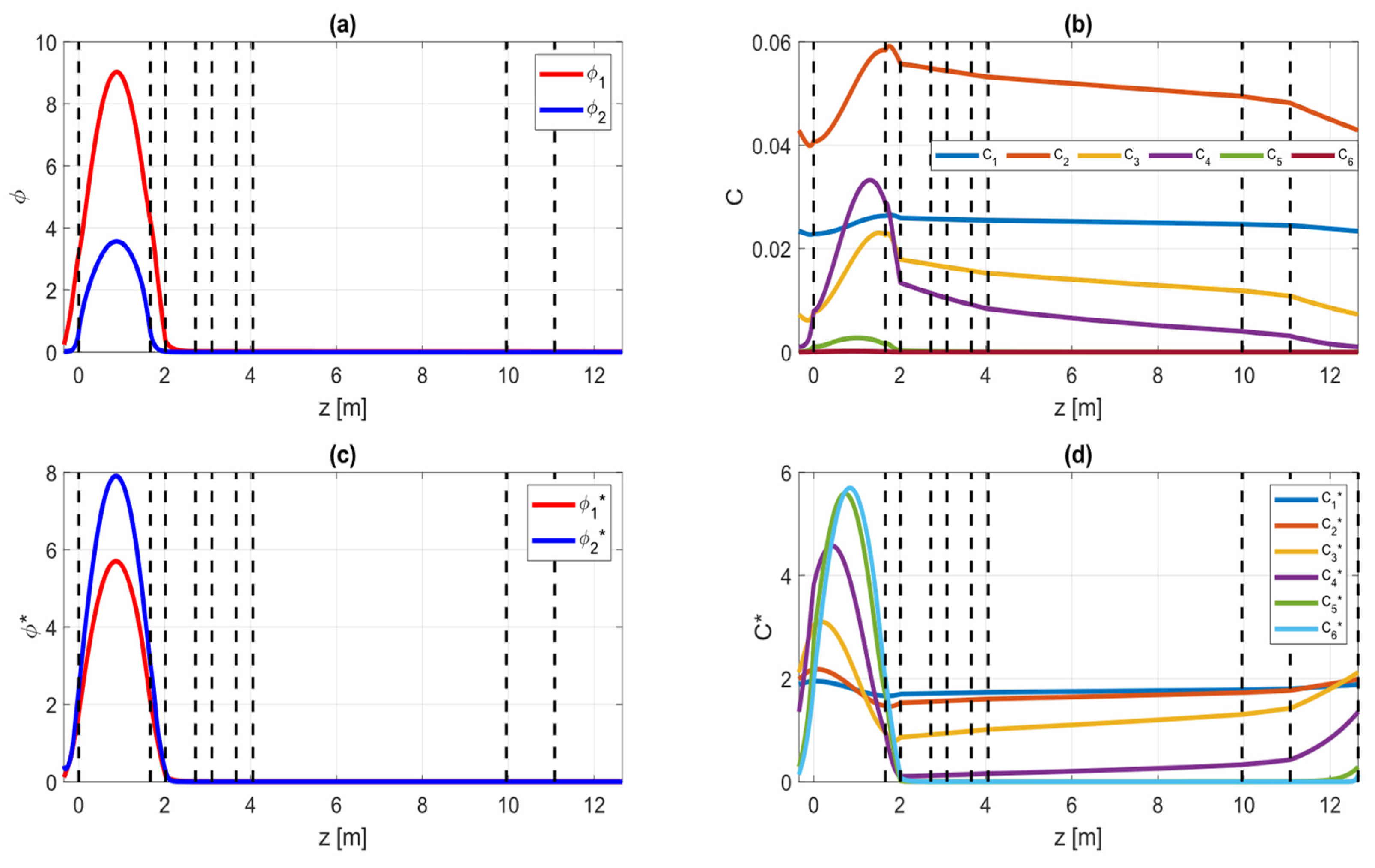
The results for both the forward and adjoint systems are shown in Figure 5.

COMSOL models are created for Equations (24) and (25) separately, using the coefficient PDE form. The two eigenvalue systems are solved using the ARPACK solver. A comparison between the value of the $k_{eff}$ for the stationary and flowing cases is summarized in

Table 7. A comparison of $k_{eff}$ for the stationary and flowing MSRE models obtained from the solution of the 1D 2G diffusion model.

	Stationary	Flowing
$k_{eff}$	1.01938	1.01714
$\Delta \rho [\mathrm{pcm}]$	-	−223

. The results for the forward and adjoint flux show that there is no significant change from the stationary fuel configuration. On the other hand, the DNP distribution at steady state flowing condition shows significant distortion from the static distribution. The long-lived DNP families exhibited more distortion compared to the short-lived families. This result is expected, as the short-lived families decay before they can drift away from their generation position. As a result of this, the short-lived DNP families decay at higher importance regions compared to the long-lived families. This effect can be shown in the adjoint DNP concentration distribution.

The total reactivity loss due to fuel circulation is estimated from the eigenvalue of the flowing-fuel configuration for both the forward and the adjoint problems was found to be −223 pcm (per cent mille), the experimental value for reactivity loss is 212 pcm [25]. The estimated reactivity loss using PROTEUS-NODAL is −222.9 pcm [23]. These results indicate the consistent 1D leakage corrected diffusion model is sufficient for reproducing the axial flux distribution and the k-eigenvalue of the MSRE configuration with sufficient accuracy. All the studied cases are solved on a single CPU core within one second. This is very efficient compared to the 3D and axisymmetric 2D models. For instance, Lindsay et al. [7] reported a run time of 5 min on a single core for the axisymmetric 2D MSRE model using a coarse axial mesh, while the 3D case required a supercomputer.

6. Conclusions

In this work, a consistent 1D leakage corrected multigroup neutron diffusion model was established for the MSR neutronics analysis. The consistent model includes an artificial leakage cross section to account for the neutron leakage in the radial direction, which cannot be directly realized in a 1D representation. The procedure of generating the leakage cross section using Serpent code is elaborated. The leakage cross section is estimated by tallying the integral net current at the geometry radial boundary surface. The ratio of the net current to the integral flux within the cell surrounded by the radial surface is the leakage cross section. The remaining cross sections are generated using the infinite spectrum. The axial flux is accounted for using the albedo boundary condition.

The consistent 1D model was verified against the reference solution obtained from 3D Serpent calculations. Four different few-group energy structures were considered in the verification procedure. The $k_{eff}$ value obtained from the diffusion model is compared to the reference value and shown with good agreement. The error in the estimated $k_{eff}$ did not decrease monotonically with increasing the energy resolution, which suggests that error cancelation mechanisms may occur for the lower resolution groups. Generally, the error in the predicted $k_{eff}$ value is comparable to values found in literature for higher spatial resolution models.

As an application for the developed model, the MSRE dynamic configuration was simulated by means of the eigenvalue analysis to estimate the reactivity loss due to fuel circulation. Both the forward and adjoint models of the problem are considered and solved for producing effective kinetics parameters. The estimated reactivity loss due to fuel circulation at the MSRE designated flow rate is 223 pcm, which is in a good agreement with the experimental values. It also verified the effect of the fuel circulation on the DNP distribution and their relative importance.

The MSRE analyses performed in this work shows that the consistent 1D leakage corrected diffusion model is sufficient to reproduce the axial flux distribution and k-eigenvalue of the MSRE, and offer the advantage of being very computationally efficient. This work is the first step in developing a fully neutronics and thermal-hydraulics-coupled model for MSR analysis, which is part of the NEUP project that aims to develop a transient reactor physics benchmark for MSR based on the experimental data of the MSRE. In the future, the consistent 1D MSR diffusion model is to be used to carry out a series of sensitivity analysis to resolve the uncertainties in the MSR design and operational parameters. The developed MSRE benchmark will serve in the development of computational tools for the MSRs.