
Nuclide Inventory Benchmark for BWR Spent Nuclear Fuel: Challenges in Evaluation of Modeling Data Assumptions and Uncertainties †


Abstract
:1. Introduction
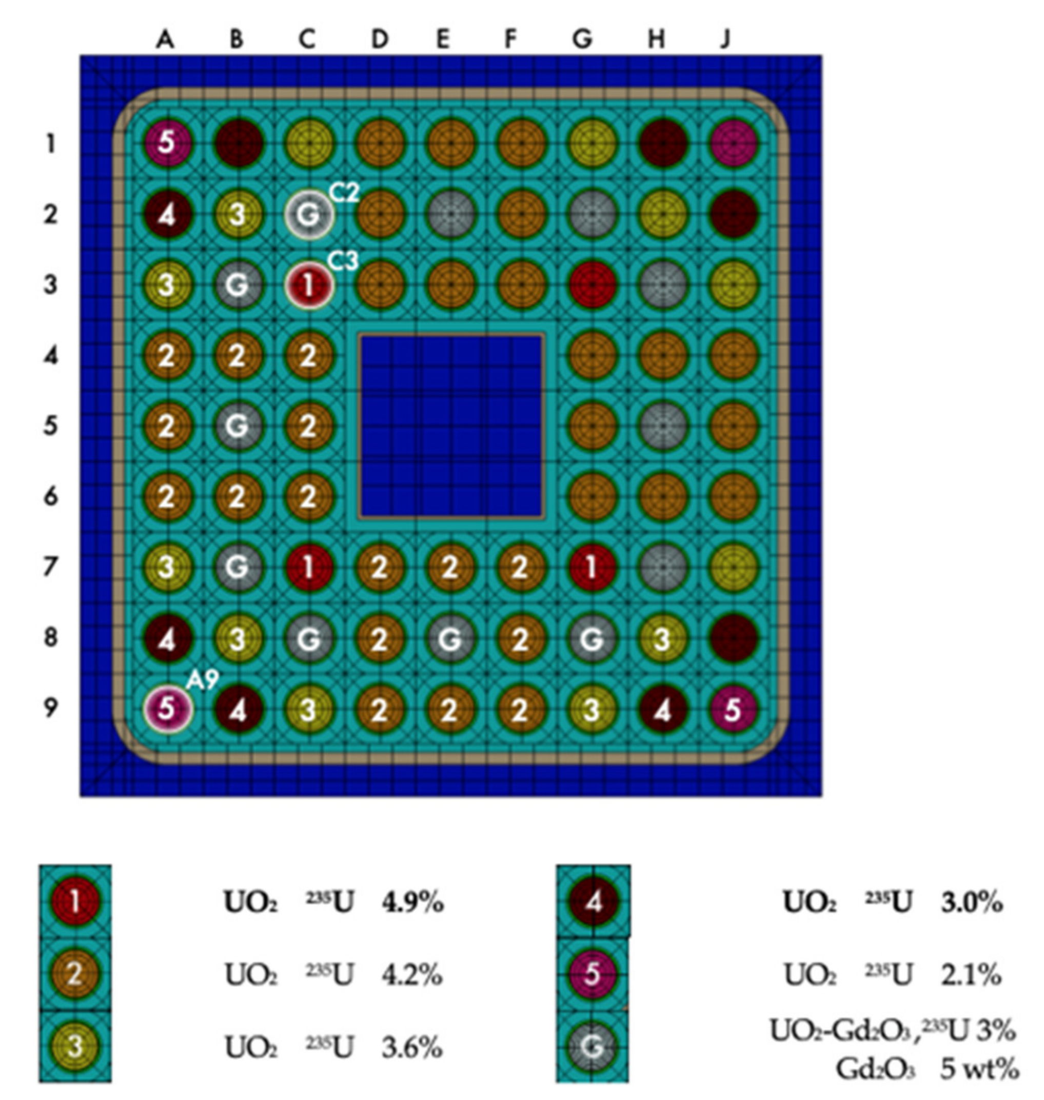
2. Overview of Experimental Data
3. Computational Models
4. Impact of Modeling Assumptions and Modeling Data Uncertainties
- Assembly and fuel rod geometry: manufacturing tolerances in assembly pitch, fuel rod pitch, fuel rod dimensions, clad thickness, and channel wall and water box dimensions;
- Material composition: manufacturing tolerances in fuel enrichment or lack of detailed initial uranium isotopic composition;
- Operating history: axial and radial intranodal void fraction distribution, temperature of fuel and coolant, density of fuel, measured sample power history and burnup, and geometry changes due to operating history (i.e., gap closure, channel/rod bow).
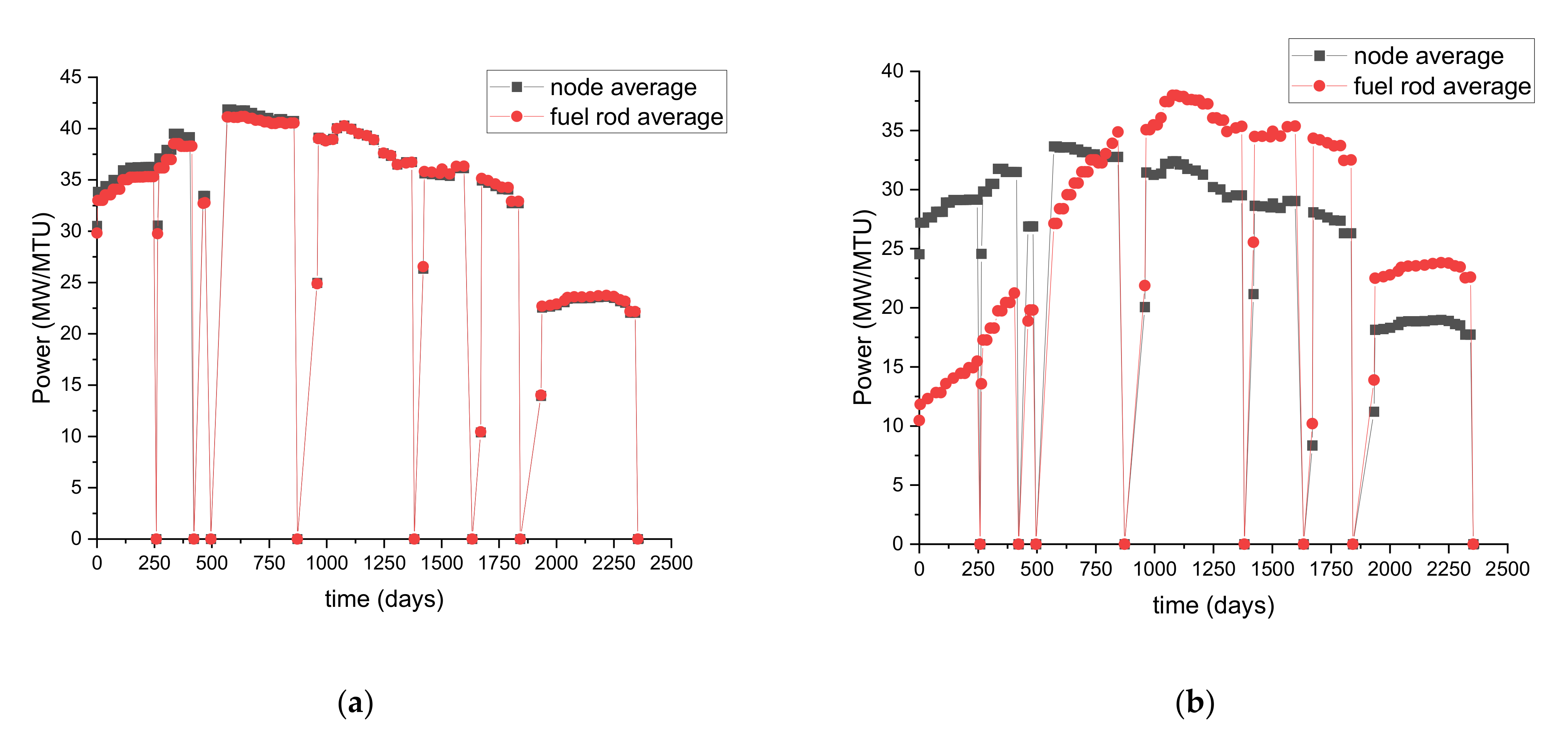
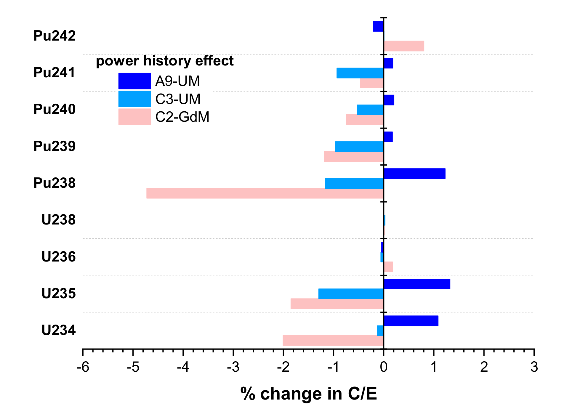
4.1. Power History
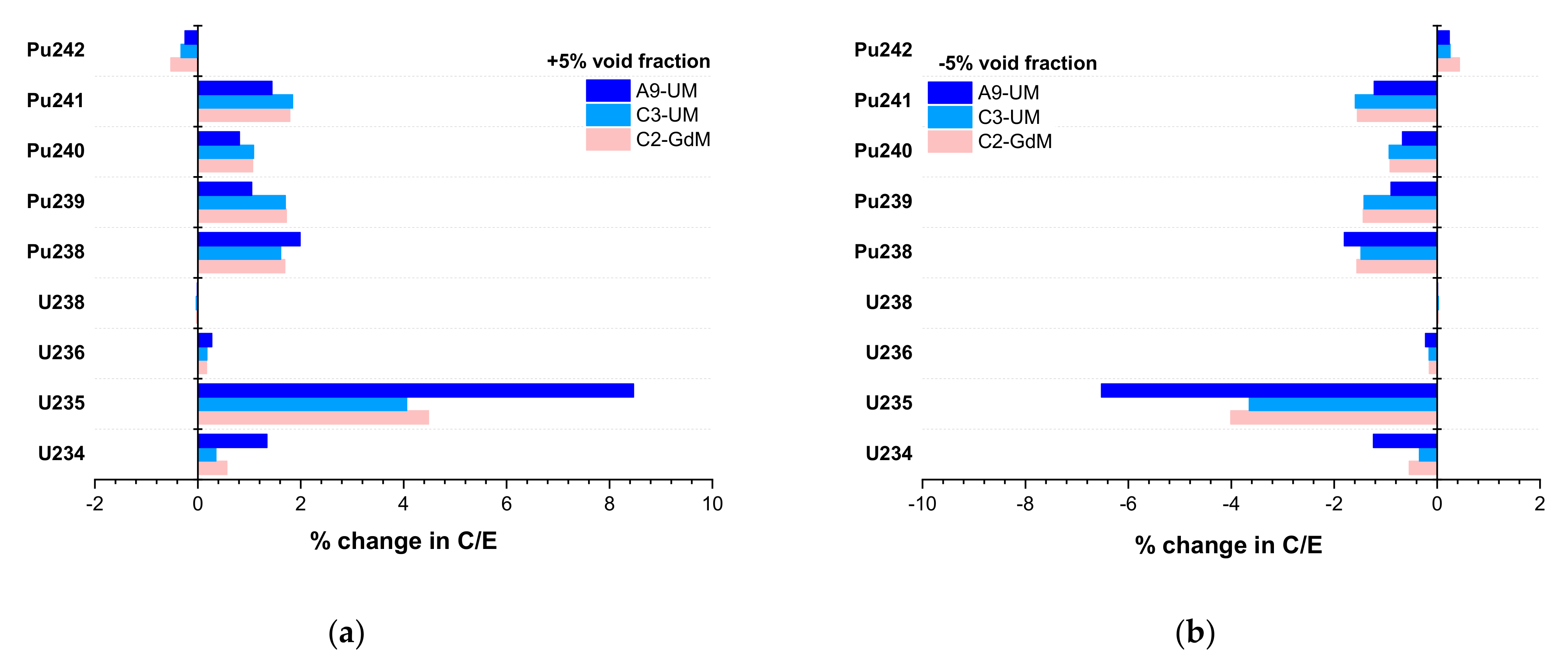
4.2. Coolant Density
4.3. Fuel Data
4.3.1. Fuel Density
4.3.2. Fuel Temperature
4.4. Geometry
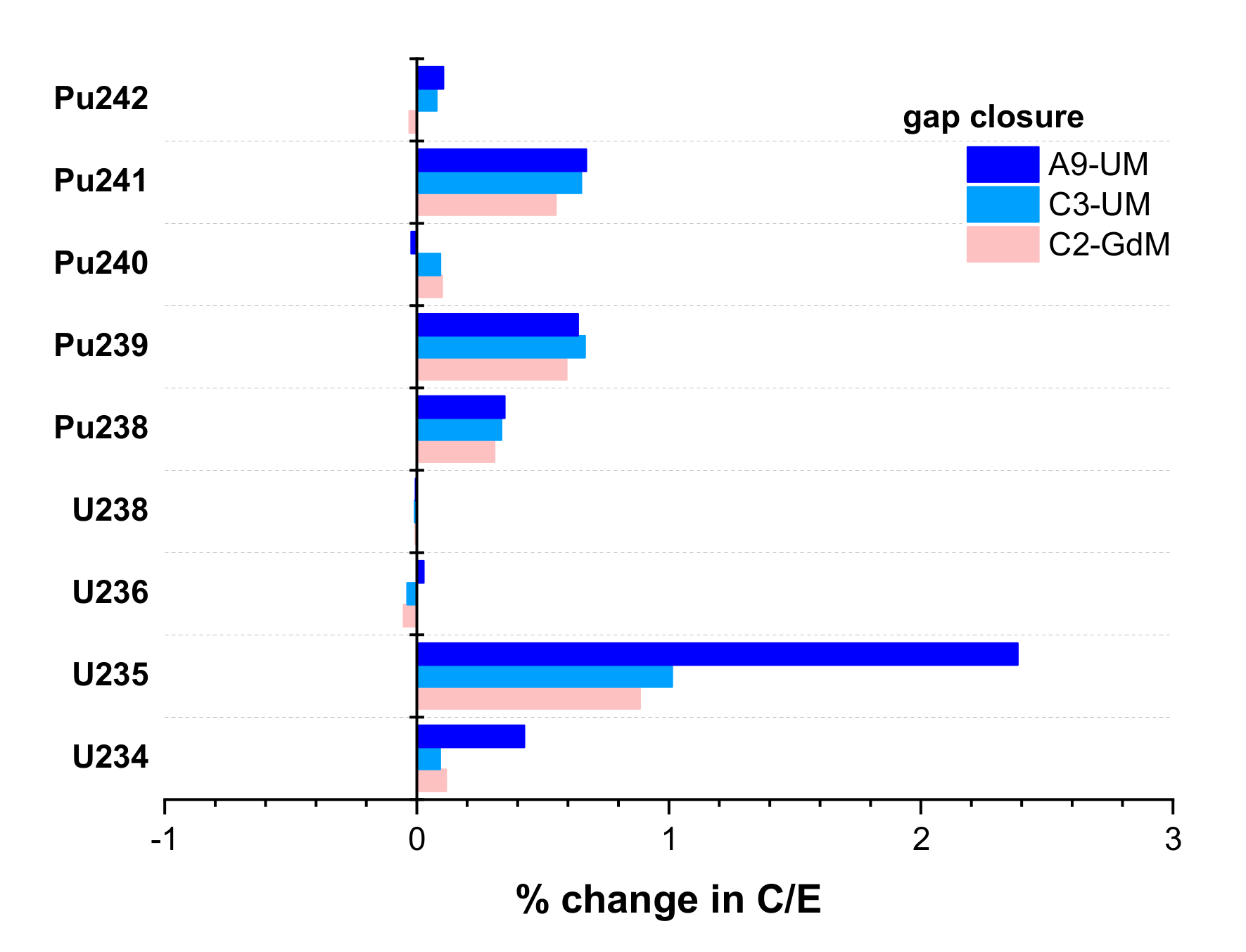
4.4.1. Gap Closure
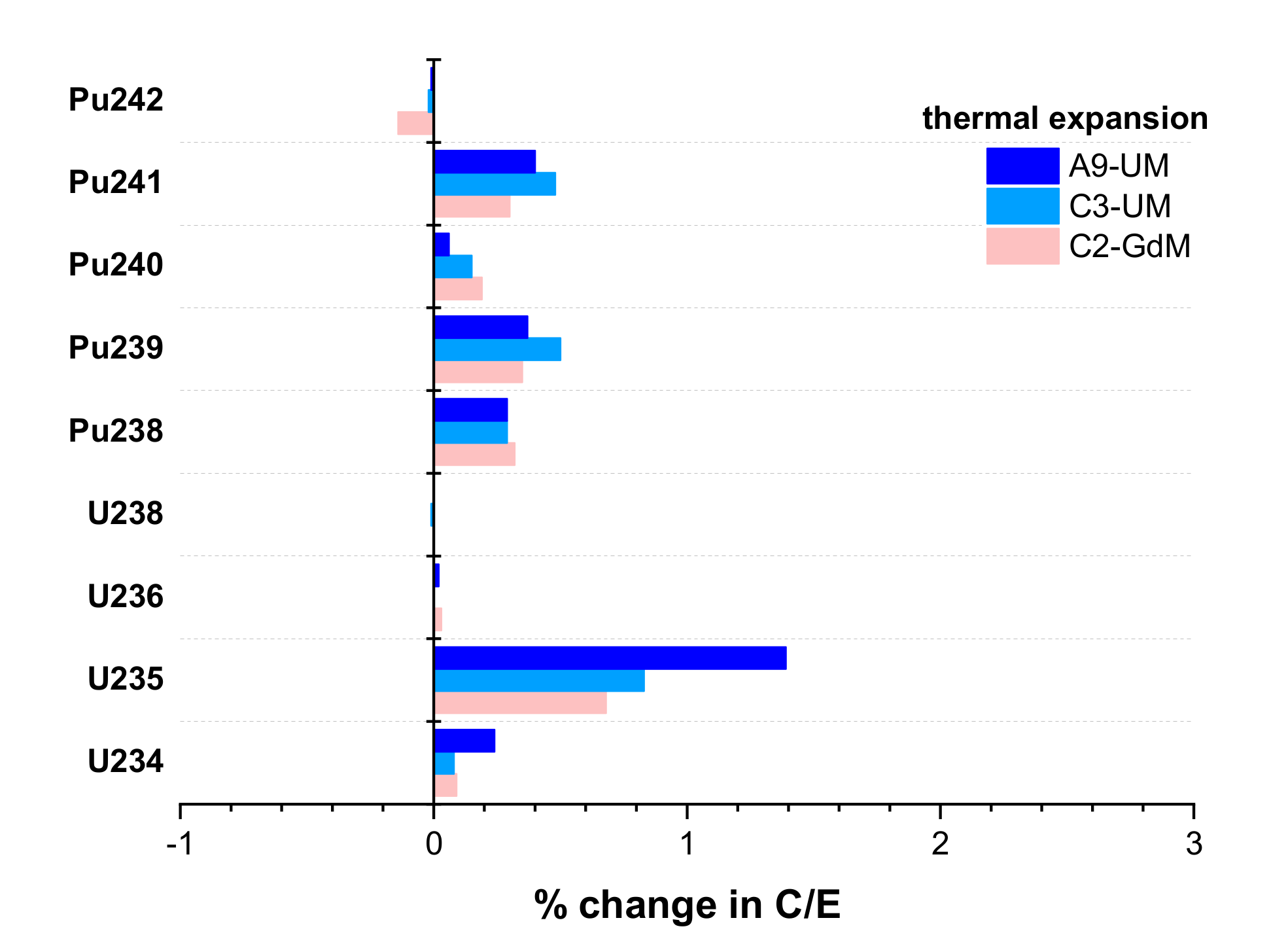
4.4.2. Thermal Expansion
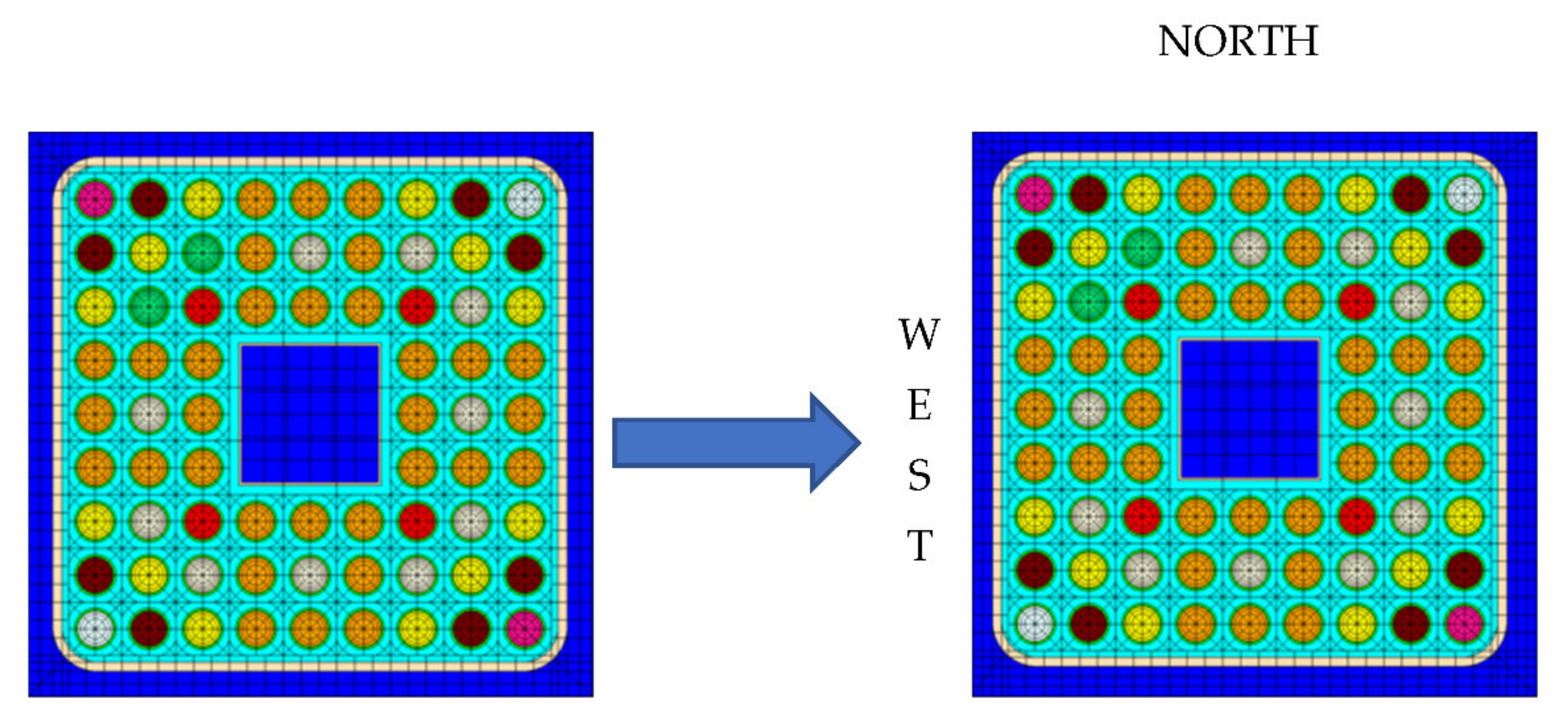
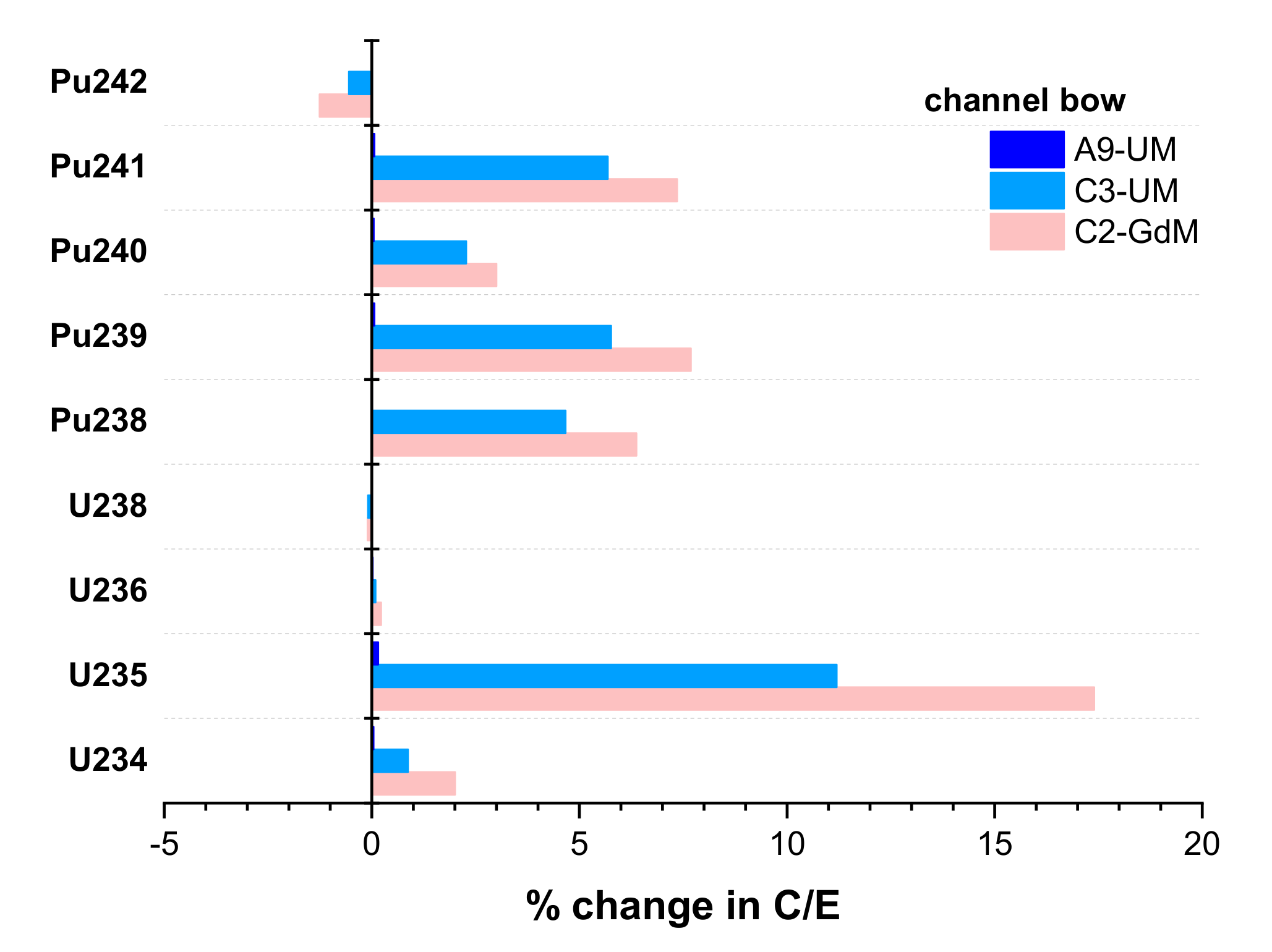
4.4.3. Channel Bow/Bulge
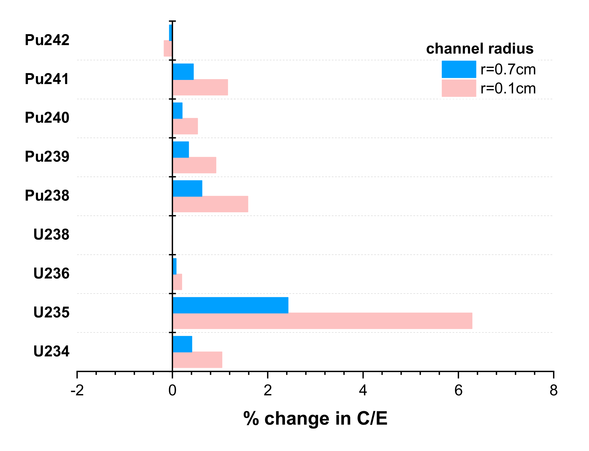
4.4.4. Channel Corner Radius
4.4.5. Geometric Manufacturing Tolerances
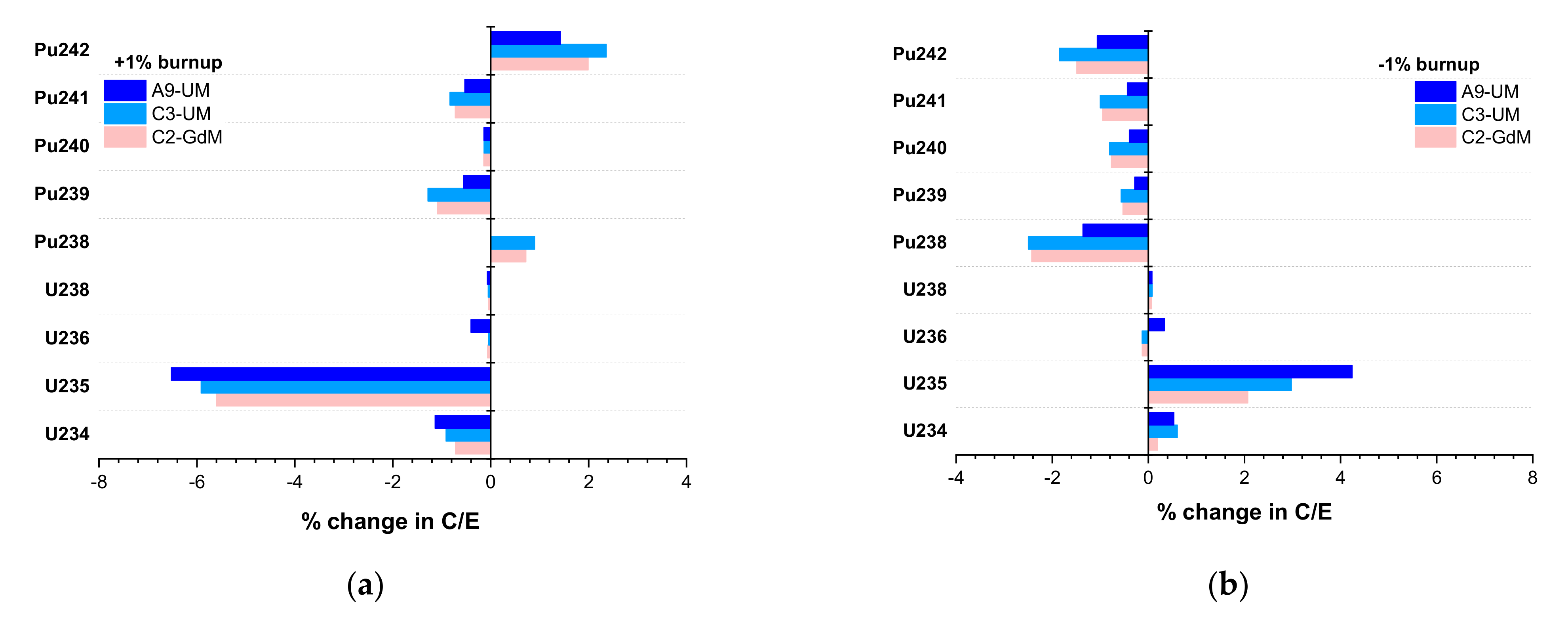
4.5. Burnup
5. Results and Discussion
5.1. Comparison between Calculation and Experiment for Nuclide Inventories
5.2. Total Uncertainty
6. Conclusions
Author Contributions
Funding
Institutional Review Board Statement
Informed Consent Statement
Data Availability Statement
Acknowledgments
Conflicts of Interest
References
- Michel-Sendis, F.; Gauld, I.; Martinez, J.S.; Alejano, C.; Bossant, M.; Boulanger, D.; Cabellos, O.; Chrapciak, V.; Conde, J.; Fast, I.; et al. SFCOMPO-2.0: An OECD NEA Database of Spent Nuclear Fuel Isotopic Assays, Reactor Design Specifications, and Operating Data. Ann. Nucl. Energy 2017, 110, 779–788. [Google Scholar] [CrossRef]
- 2. Evaluation Guide for the Evaluated Spent Nuclear Fuel Assay Database (SFCOMPO), 2016. NEA/NSC/R(2015), Nuclear Energy Agency, France. Available online: https://www.oecd-nea.org/science/docs/2015/nsc-r2015-8.pdf (accessed on 10 December 2021).
- Ilas, G.; Gauld, I.C.; Ortego, P.; Tsuda, S. SFCOMPO database of spent nuclear fuel assay data-the next frontier. In EPJ Web of Conference; EDP Sciences: Les Ulis, France, 2020. Available online: https://www.osti.gov/biblio/1649454 (accessed on 10 December 2021)ISBN 978-1-5272-6447-2.
- International Reactor Physics Experiment Evaluation (IRPhE) Project. Nuclear Energy Agency, France. 2016. Available online: https://www.oecd-nea.org/science/wprs/irphe/ (accessed on 10 December 2021).
- Briggs, J.B.; Scott, L.; Nouri, A. The International Criticality Safety Benchmark Evaluation Project. Nucl. Sci. Eng. 2003, 145, 1–10. [Google Scholar] [CrossRef]
- Wieselquist, W.A.; Lefebvre, R.A.; Jessee, M.A. SCALE Code System; ORNL/TM-2005/39, Version 6.2.4; Oak Ridge National Laboratory: Oak Ridge, TN, USA, 2020. Available online: https://www.ornl.gov/file/scale-62-manual/display (accessed on 10 December 2021).
- Okumura, K.; Kaneko, K.; Tsuchihashi, K. SRAC95, General Purpose Neutronics Code System; JAERI-Data/Code 96-015; Japan Atomic Energy Research Institute: Tokyo, Japan, 1996.
- Suzuki, M.; Yamamoto, T.; Fukaya, H.; Suyama, K.; Uchiyama, G. Lattice Physics Analysis of Measured Isotopic Compositions of Irradiated BWR 9 × 9 UO2 fuel. J. Nucl. Sci. Technol. 2013, 50, 1161–1176. [Google Scholar] [CrossRef]
- Okumura, K.; Mori, T.; Nakagawa, M.; Kaneko, K. Validation of a continuous-energy Monte Carlo Burn-Up Code MVP-BURN and its Application to Analysis of Post Irradiation Experiment. J. Nucl. Sci. Technol. 2020, 37, 128. [Google Scholar] [CrossRef]
- Jessee, M.A.; Wieselquist, W.A.; Mertyurek, U.; Kim, K.S.; Evans, T.M.; Hamilton, S.P.; Gentry, C. Lattice physics calculations using the embedded self-shielding method in Polaris, Part I: Methods and implementation. Ann. Nucl. Energy 2021, 150, 107830. [Google Scholar] [CrossRef]
- Mertyurek, U.; Jessee, M.A.; Betzler, B.R. Lattice physics calculations using the embedded self-shielding method in Polaris, Part II: Benchmark assessment. Ann. Nucl. Energy 2021, 150, 107829. [Google Scholar] [CrossRef]
- Gauld, I.C.; Radulescu, G.; Ilas, G.; Murphy, B.D.; Williams, M.L.; Wiarda, D. Isotopic Depletion and Decay Methods and Analysis Capabilities in SCALE. Nucl. Technol. 2011, 174, 169. [Google Scholar] [CrossRef]
- Gauld, I.C.; Mertyurek, U. Void Fraction Distribution in BWR Fuel Assembly and Evaluation of Subchannel Code. J. Nucl. Sci. Technol. 1995, 32, 629–640. [Google Scholar]
- Radulescu, H.R. Limerick Unit 1 Radiochemical Assay Comparisons to SAS2H Calculations; CAL-DSU-NU-000002 Rev 00A; Office of Civilian Radioactive Waste Management, US Department of Energy: Washington, DC, USA, 2003.
- O’Donnell, G.M.; Scott, H.H.; Meyer, R.O. A New Comparative Analysis of LWR Fuel Designs, NUREG-1754, US Nuclear Regulatory Commission. 2001. Available online: https://www.nrc.gov/docs/ML0136/ML013650469.pdf (accessed on 10 December 2021).
- De Kruijf, W.J.M.; Janssen, A.J. The Effective Fuel Temperature to Be Used for Calculating Resonance Absorption in a 238UO2 Lump with a Nonuniform Temperature Profile. Nucl. Sci. Eng. 1996, 123, 121–135. [Google Scholar] [CrossRef]
- Palmtag, S. Investigation of Thermal Expansion Effects in MPACT; CASL-U-2016-1015-000; Oak Ridge National Laboratory: Oak Ridge, TN, USA, 2016.
- Garzarolli, F.; Adamson, R.; Rudling, P.; Strasser, A. BWR Fuel Channel Distortion; ZIRAT16 Special Topical Report; ANT International: Molnlycke, Sweden, 2011; Available online: https://www.antinternational.com/docs/samples/FM/04/ZIRAT16_STR_ChannelDistortion_sample1.pdf (accessed on 10 December 2021).
- Kelly, D.J. Depletion of a BWR Lattice Using the RACER Continuous Energy Monte Carlo Code. In Proceedings of the International Conference on Mathematics and Computations, Reactor Physics, and Environmental Analyses, Portland, OR, USA, 30 April–4 May 1995. [Google Scholar]
- Gauld, I.C.; Mertyurek, U. Validation of BWR spent nuclear fuel isotopic predictions with applications to burnup credit. Nucl. Eng. Des. 2019, 345, 110. [Google Scholar] [CrossRef]
- Gauld, I.C.; Mertyurek, U. Margins for Uncertainty in the Predicted Spent Fuel Isotopic Inventories for BWR Burnup Credit, NUREG/CR-7251, US Nuclear Regulatory Commission. 2018. Available online: https://www.nrc.gov/reading-rm/doc-collections/nuregs/contract/cr7251/ (accessed on 10 December 2021).
- Rochman, D.; Vasiliev, A.; Ferroukhi, H.; Hursin, M. Analysis for the ARIANE GU1 sample: Nuclide inventory and decay heat. Ann. Nucl. Energy 2021, 160, 108359. [Google Scholar] [CrossRef]
- Williams, M.; Ilas, G.; Jessee, M.A.; Rearden, B.T.; Wiarda, D.; Zwermann, W.; Gallner, L.; Klein, M.; Krzykacz-Hausmann, B.; Pautz, A. A statistical sampling method for uncertainty analysis with SCALE and XSUSA. Nucl. Technol. 2013, 183, 515–526. [Google Scholar] [CrossRef]
- Ilas, G.; Liljenfeldt, H. Decay heat uncertainty for BWR used fuel due to modeling and nuclear data uncertainties. Nucl. Eng. Des. 2017, 319, 176–184. [Google Scholar] [CrossRef]


| Sample ID | 2F1ZN2-C2-GdT | 2F1ZN2-C3-UT | 2F1ZN3-C2-GdM | 2F1ZN3-C3-UM | 2F1ZN3-A9-UM |
|---|---|---|---|---|---|
| Fuel type | UO2-Gd2O3 | UO2 | UO2-Gd2O3 | UO2 | UO2 |
| Enrichment (%) | 3.0 | 4.9 | 3.0 | 4.9 | 2.1 |
| Gd loading (wt % Gd2O3) | 5.0 | 0 | 5.0 | 0 | 0 |
| Avg. void fraction (%) | 74 | 74 | 38 | 38 | 38 |
| Burnup 1 (GWd/MTU) | 29.0 | 38.9 | 57.7 | 68.4 | 68.0 |
| Sample ID | Measured [7,9] | Calculated SRAC [9] | Calculated MVP-BURN [9] | Calculated Polaris |
|---|---|---|---|---|
| 2F1ZN2-C2-GdT | 27.89 | 28.44 | 28.70 | 28.17 |
| 2F1ZN2-C3-UT | 38.15 | 39.05 | 38.77 | 37.39 |
| 2F1ZN3-C2-GdM | 54.45 | 53.82 | 54.35 | 55.00 |
| 2F1ZN3-C3-UM | 68.42 | 68.06 | 67.61 | 67.73 |
| 2F1ZN3-A9-UM | 64.18 | 60.28 | 61.29 | 63.54 |
| Sample ID | 2F1ZN2-C2-GdT | 2F1ZN2-C3-UT | 2F1ZN3-C2-GdM | 2F1ZN3-C3-UM | 2F1ZN3-A9-UM | |||
|---|---|---|---|---|---|---|---|---|
| Fuel type | UO2-Gd2O3 | UO2 | UO2-Gd2O3 | UO2 | UO2 | |||
| Burnup 1 (GWd/MTU) | 29.0 | 38.9 | 57.7 | 68.4 | 68.0 | |||
| Nuclide | C/E-1 (%) | C/E-1 (%) | C/E-1 (%) | C/E-1 (%) | C/E-1 (%) | Avg 2 (%) | Stdev 3 (%) | Exp. uncert. 4 (%) |
| 234U | 8.7 | −3.8 | 11.0 | 3.4 | 18.6 | 7.6 | 8.4 | <1.4 |
| 235U | 3.2 | 4.4 | 6.4 | 7.6 | −3.1 | 3.7 | 4.1 | 4 |
| 236U | 2.1 | 2.4 | 2.8 | 3.3 | 3.5 | 2.8 | 0.6 | <0.2 |
| 238U | −0.2 | −0.2 | −0.2 | −0.2 | −0.1 | −0.2 | 0.0 | <0.2 |
| 238Pu | 8.1 | 2.6 | 18.0 | 6.5 | 10.7 | 9.2 | 5.7 | <0.5 |
| 239Pu | 6.1 | 4.0 | −5.1 | −3.7 | −9.0 | −1.5 | 6.4 | <0.2 |
| 240Pu | 0.3 | −3.5 | −2.1 | −2.3 | 0.4 | −1.4 | 1.7 | <0.2 |
| 241Pu | 3.5 | 0.7 | −5.3 | −3.9 | −9.4 | −2.9 | 5.1 | <0.2 |
| 242Pu | 3.0 | −1.9 | 1.9 | 3.2 | 3.6 | 2.0 | 2.2 | <0.2 |
| 143Nd | 2.0 | 2.4 | 5.4 | 5.1 | 2.6 | 3.5 | 1.6 | <0.3 |
| 145Nd | 0.5 | 0.7 | 2.3 | 2.1 | 1.5 | 1.4 | 0.8 | <0.3 |
| 146Nd | −1.4 | −1.3 | −2.1 | −1.9 | −2.7 | −1.9 | 0.6 | 0.3 |
| 148Nd | −0.3 | −0.2 | 0.2 | 0.1 | −0.5 | −0.1 | 0.3 | <0.3 |
| 133Cs | n/a | 1.4 | −1.1 | 2.0 | 1.9 | 1.1 | 1.3 | 4.8 |
| 137Cs | −6.2 | −8.3 | −13.4 | −11.5 | −8.9 | −9.6 | 2.8 | <4 |
| 151Eu | −31.0 | −7.5 | −47.3 | −36.6 | −38.7 | −32.2 | 15.0 | 3.8 |
| 153Eu | 11.2 | 5.3 | 3.7 | 4.6 | 0.2 | 5.0 | 4.0 | 2.6 |
| 155Eu | 15.6 | 6.7 | −2.4 | −3.1 | −8.0 | 1.8 | 9.4 | <6 |
| 155Gd | −6.7 | 14.7 | −3.0 | 10.3 | 4.5 | 4.0 | 8.9 | 1.4 |
| 147Sm | −0.9 | −1.3 | 0.1 | 0.6 | 1.5 | 0.0 | 1.1 | 2.1 |
| 149Sm | 5.2 | 14.3 | −5.8 | 2.2 | −14.7 | 0.3 | 11.0 | 3.7 |
| 150Sm | 1.4 | 4.0 | 0.3 | 4.0 | 2.4 | 2.4 | 1.6 | 2.2 |
| 151Sm | 2.1 | 3.9 | −6.0 | −2.7 | −9.1 | −2.3 | 5.4 | 1.6 |
| 152Sm | 6.0 | 7.0 | 9.7 | 11.5 | 9.3 | 8.7 | 2.2 | 1.9 |
| 95Mo | −7.6 | −4.4 | −4.9 | −4.6 | −3.2 | −4.9 | 1.6 | 4.5 |
| 99Tc | 37.4 | 39.9 | 45.3 | 42.1 | 49.4 | 42.8 | 4.7 | 3.5 |
| 101Ru | −3.1 | −2.1 | −1.4 | −3.2 | −3.3 | −2.6 | 0.8 | 3.8 |
| 103Rh | 0.3 | 0.9 | 5.2 | 2.4 | 1.1 | 2.0 | 2.0 | 3.7 |
| Nuclide | Uncertainties (%) | ||||||||
|---|---|---|---|---|---|---|---|---|---|
| C/E-1 (%) | Burnup | Void Fraction | Fuel Temp. | Thermal Expansion | Power History | Fuel Density | Exp. | Total | |
| 234U | 11.03 | 0.46 | 0.56 | 0.76 | 0.09 | 2.01 | 0.27 | 1.55 | 2.76 |
| 235U | 6.35 | 3.84 | 4.25 | 3.16 | 0.68 | 1.85 | 2.01 | 0.32 | 7.13 |
| 236U | 2.80 | 0.10 | 0.16 | 0.17 | 0.03 | 0.18 | 0.07 | 0.21 | 0.38 |
| 238U | −0.17 | 0.05 | 0.02 | 0.02 | 0.00 | 0.01 | 0.01 | 0.20 | 0.21 |
| 238Pu | 17.99 | 1.57 | 1.63 | 1.05 | 0.32 | 4.72 | 0.83 | 0.59 | 5.45 |
| 239Pu | −5.08 | 0.81 | 1.58 | 1.22 | 0.35 | 1.18 | 0.82 | 0.19 | 2.62 |
| 240Pu | −2.06 | 0.46 | 0.99 | 0.37 | 0.19 | 0.75 | 0.43 | 0.20 | 1.47 |
| 241Pu | −5.27 | 0.84 | 1.67 | 1.34 | 0.30 | 0.47 | 0.82 | 0.19 | 2.51 |
| 242Pu | 1.86 | 1.74 | 0.48 | 0.15 | 0.14 | 0.80 | 0.25 | 0.20 | 2.01 |
| 143Nd | 5.36 | 0.61 | 1.25 | 0.92 | 0.21 | 0.61 | 0.59 | 0.32 | 1.90 |
| 145Nd | 2.32 | 0.69 | 0.01 | 0.11 | 0.01 | 0.06 | 0.01 | 0.31 | 0.76 |
| 146Nd | −2.11 | 1.12 | 0.07 | 0.17 | 0.00 | 0.01 | 0.03 | 0.29 | 1.18 |
| 148Nd | 0.21 | 0.99 | 0.02 | 0.02 | 0.00 | 0.19 | 0.01 | 0.30 | 1.05 |
| 133Cs | −1.09 | 0.71 | 0.01 | 0.13 | 0.01 | 0.07 | 0.00 | 3.07 | 3.15 |
| 137Cs | −13.38 | 0.86 | 0.02 | 0.00 | 0.00 | 0.93 | 0.01 | 3.46 | 3.69 |
| 151Eu | −47.29 | 0.52 | 0.79 | 0.75 | 0.19 | 0.19 | 0.53 | 1.32 | 1.88 |
| 153Eu | 3.69 | 0.78 | 0.15 | 0.44 | 0.03 | 0.01 | 0.11 | 2.18 | 2.36 |
| 155Eu | −2.43 | 0.89 | 0.40 | 1.53 | 0.09 | 0.73 | 0.20 | 5.85 | 6.18 |
| 155Gd | −2.98 | 0.56 | 0.54 | 0.98 | 0.14 | 0.29 | 0.35 | 8.25 | 8.35 |
| 147Sm | 0.05 | 0.07 | 0.05 | 0.50 | 0.02 | 1.40 | 0.01 | 1.80 | 2.33 |
| 149Sm | −5.84 | 0.70 | 1.07 | 1.03 | 0.28 | 11.66 | 0.71 | 3.20 | 12.23 |
| 150Sm | 0.27 | 0.96 | 0.24 | 0.09 | 0.04 | 1.12 | 0.12 | 1.80 | 2.35 |
| 151Sm | −5.96 | 0.91 | 1.37 | 1.30 | 0.34 | 0.11 | 0.92 | 2.26 | 3.23 |
| 152Sm | 9.73 | 0.68 | 0.39 | 0.00 | 0.15 | 0.92 | 0.30 | 1.76 | 2.16 |
| 95Mo | −4.92 | 0.72 | 0.07 | 0.01 | 0.01 | 0.11 | 0.03 | 2.09 | 2.22 |
| 99Tc | 45.28 | 1.08 | 0.03 | 0.16 | 0.01 | 0.16 | 0.02 | 3.49 | 3.66 |
| 101Ru | −1.39 | 0.91 | 0.05 | 0.04 | 0.01 | 0.09 | 0.03 | 1.97 | 2.18 |
| 103Rh | 5.23 | 0.51 | 0.37 | 1.04 | 0.04 | 0.40 | 0.14 | 2.10 | 2.47 |
| Nuclide | Uncertainties (%) | ||||||||
|---|---|---|---|---|---|---|---|---|---|
| C/E-1 (%) | Burnup | Void Fraction | Fuel Temp. | Thermal Expansion | Power History | Fuel Density | Exp. | Total | |
| 234U | 3.42 | 0.76 | 0.35 | 0.64 | 0.08 | 0.12 | 0.16 | 1.45 | 1.80 |
| 235U | 7.58 | 4.45 | 3.86 | 2.88 | 0.83 | 1.29 | 1.77 | 0.32 | 6.97 |
| 236U | 3.33 | 0.09 | 0.17 | 0.19 | 0.00 | 0.06 | 0.06 | 0.21 | 0.35 |
| 238U | −0.20 | 0.07 | 0.03 | 0.02 | 0.01 | 0.02 | 0.01 | 0.20 | 0.22 |
| 238Pu | 6.47 | 1.70 | 1.55 | 1.22 | 0.29 | 1.17 | 0.77 | 0.53 | 3.01 |
| 239Pu | −3.73 | 0.92 | 1.56 | 1.25 | 0.50 | 0.96 | 0.94 | 0.19 | 2.64 |
| 240Pu | −2.27 | 0.47 | 1.01 | 0.42 | 0.15 | 0.53 | 0.44 | 0.20 | 1.40 |
| 241Pu | −3.93 | 0.92 | 1.72 | 1.40 | 0.48 | 0.93 | 0.89 | 0.19 | 2.77 |
| 242Pu | 3.19 | 2.11 | 0.29 | 0.24 | 0.02 | 0.01 | 0.25 | 0.21 | 2.16 |
| 143Nd | 5.13 | 0.63 | 1.26 | 0.93 | 0.27 | 0.59 | 0.60 | 0.32 | 1.93 |
| 145Nd | 2.06 | 0.61 | 0.04 | 0.10 | 0.00 | 0.05 | 0.02 | 0.31 | 0.69 |
| 146Nd | −1.87 | 1.18 | 0.06 | 0.16 | 0.03 | 0.14 | 0.02 | 0.29 | 1.24 |
| 148Nd | 0.07 | 1.00 | 0.02 | 0.02 | 0.01 | 0.12 | 0.01 | 0.30 | 1.05 |
| 133Cs | 2.04 | 0.67 | 0.01 | 0.13 | 0.00 | 0.07 | 0.02 | 4.90 | 4.95 |
| 137Cs | −11.48 | 0.88 | 0.01 | 0.00 | 0.00 | 0.07 | 0.01 | 3.54 | 3.65 |
| 151Eu | −36.63 | 0.58 | 0.92 | 0.88 | 0.26 | 0.63 | 0.59 | 0.82 | 1.86 |
| 153Eu | 4.56 | 0.85 | 0.08 | 0.40 | 0.07 | 0.18 | 0.06 | 0.52 | 1.10 |
| 155Eu | −3.11 | 0.96 | 0.35 | 1.44 | 0.10 | 0.31 | 0.21 | 0.21 | 1.81 |
| 155Gd | 10.27 | 1.08 | 0.42 | 1.61 | 0.13 | 0.38 | 0.26 | 5.81 | 6.09 |
| 147Sm | 0.61 | 0.19 | 0.02 | 0.48 | 0.00 | 0.04 | 0.06 | 1.21 | 1.32 |
| 149Sm | 2.24 | 0.71 | 1.06 | 1.04 | 0.35 | 0.16 | 0.73 | 1.53 | 2.39 |
| 150Sm | 4.04 | 0.98 | 0.27 | 0.11 | 0.05 | 0.24 | 0.14 | 1.25 | 1.64 |
| 151Sm | −2.66 | 0.88 | 1.38 | 1.32 | 0.40 | 0.93 | 0.89 | 1.46 | 2.89 |
| 152Sm | 11.48 | 0.68 | 0.41 | 0.07 | 0.12 | 0.28 | 0.34 | 1.23 | 1.53 |
| 95Mo | −4.56 | 0.69 | 0.08 | 0.03 | 0.01 | 0.05 | 0.04 | 4.29 | 4.35 |
| 99Tc | 42.12 | 1.02 | 0.05 | 0.16 | 0.01 | 0.01 | 0.03 | 4.97 | 5.08 |
| 101Ru | −3.20 | 0.89 | 0.06 | 0.05 | 0.01 | 0.08 | 0.03 | 3.68 | 3.79 |
| 103Rh | 2.39 | 0.39 | 0.38 | 1.08 | 0.10 | 0.18 | 0.14 | 3.79 | 3.99 |
| Nuclide | Uncertainties (%) | ||||||||
|---|---|---|---|---|---|---|---|---|---|
| C/E-1 (%) | Burnup | Void Fraction | Fuel Temp. | Thermal Expansion | Power History | Fuel Density | Exp. | Total | |
| 234U | 18.60 | 0.83 | 1.29 | 1.22 | 0.24 | 1.08 | 0.32 | 1.66 | 2.82 |
| 235U | −3.08 | 5.38 | 7.50 | 4.58 | 1.39 | 1.32 | 1.75 | 3.88 | 11.31 |
| 236U | 3.46 | 0.37 | 0.25 | 0.03 | 0.02 | 0.04 | 0.03 | 0.21 | 0.50 |
| 238U | −0.08 | 0.07 | 0.01 | 0.01 | 0.00 | 0.00 | 0.00 | 0.20 | 0.21 |
| 238Pu | 10.69 | 0.68 | 1.90 | 1.03 | 0.29 | 1.23 | 0.63 | 0.55 | 2.72 |
| 239Pu | −9.00 | 0.42 | 0.97 | 0.85 | 0.37 | 0.17 | 0.43 | 0.18 | 1.50 |
| 240Pu | 0.43 | 0.27 | 0.74 | 0.28 | 0.06 | 0.20 | 0.26 | 0.20 | 0.93 |
| 241Pu | −9.40 | 0.48 | 1.33 | 1.09 | 0.40 | 0.18 | 0.48 | 0.18 | 1.91 |
| 242Pu | 18.60 | 0.83 | 1.29 | 1.22 | 0.24 | 1.08 | 0.32 | 0.21 | 1.32 |
| 143Nd | 2.56 | 0.50 | 1.83 | 1.20 | 0.37 | 0.32 | 0.50 | 0.31 | 2.37 |
| 145Nd | 1.48 | 0.64 | 0.15 | 0.22 | 0.04 | 0.03 | 0.01 | 0.30 | 0.76 |
| 146Nd | −2.72 | 1.15 | 0.14 | 0.19 | 0.04 | 0.09 | 0.01 | 0.29 | 1.21 |
| 148Nd | −0.49 | 1.01 | 0.03 | 0.02 | 0.01 | 0.07 | 0.00 | 0.30 | 1.05 |
| 133Cs | 1.90 | 0.66 | 0.10 | 0.22 | 0.03 | 0.04 | 0.01 | 3.57 | 3.64 |
| 137Cs | −8.94 | 0.91 | 0.01 | 0.00 | 0.00 | 0.29 | 0.00 | 3.64 | 3.77 |
| 151Eu | −38.66 | 0.31 | 0.64 | 0.62 | 0.18 | 0.01 | 0.31 | 0.86 | 1.33 |
| 153Eu | 0.17 | 0.66 | 0.23 | 0.44 | 0.10 | 0.03 | 0.04 | 0.70 | 1.09 |
| 155Eu | −8.00 | 0.66 | 0.35 | 1.17 | 0.11 | 0.09 | 0.10 | 5.52 | 5.70 |
| 155Gd | 4.54 | 0.74 | 0.41 | 1.32 | 0.12 | 0.07 | 0.12 | 1.36 | 2.08 |
| 147Sm | 1.45 | 0.02 | 0.32 | 0.72 | 0.09 | 0.41 | 0.03 | 1.22 | 1.51 |
| 149Sm | −14.65 | 0.49 | 0.56 | 0.56 | 0.19 | 2.22 | 0.29 | 1.79 | 3.03 |
| 150Sm | 2.39 | 0.82 | 0.47 | 0.25 | 0.09 | 0.18 | 0.14 | 1.33 | 1.67 |
| 151Sm | −9.12 | 0.45 | 0.93 | 0.91 | 0.26 | 0.05 | 0.45 | 1.91 | 2.41 |
| 152Sm | 9.26 | 0.67 | 0.24 | 0.03 | 0.06 | 0.18 | 0.25 | 1.20 | 1.43 |
| 95Mo | −3.18 | 0.72 | 0.04 | 0.06 | 0.01 | 0.04 | 0.00 | 2.23 | 2.34 |
| 99Tc | 49.43 | 1.11 | 0.08 | 0.28 | 0.03 | 0.04 | 0.02 | 3.59 | 3.76 |
| 101Ru | −3.32 | 0.89 | 0.04 | 0.06 | 0.00 | 0.07 | 0.03 | 2.13 | 2.31 |
| 103Rh | 1.08 | 0.33 | 0.57 | 1.15 | 0.15 | 0.07 | 0.08 | 1.92 | 2.34 |
Publisher’s Note: MDPI stays neutral with regard to jurisdictional claims in published maps and institutional affiliations. |
© 2022 by the authors. Licensee MDPI, Basel, Switzerland. This article is an open access article distributed under the terms and conditions of the Creative Commons Attribution (CC BY) license (https://creativecommons.org/licenses/by/4.0/).
Share and Cite
Mertyurek, U.; Ilas, G. Nuclide Inventory Benchmark for BWR Spent Nuclear Fuel: Challenges in Evaluation of Modeling Data Assumptions and Uncertainties. J. Nucl. Eng. 2022, 3, 18-36. https://doi.org/10.3390/jne3010003
Mertyurek U, Ilas G. Nuclide Inventory Benchmark for BWR Spent Nuclear Fuel: Challenges in Evaluation of Modeling Data Assumptions and Uncertainties. Journal of Nuclear Engineering. 2022; 3(1):18-36. https://doi.org/10.3390/jne3010003
Chicago/Turabian StyleMertyurek, Ugur, and Germina Ilas. 2022. "Nuclide Inventory Benchmark for BWR Spent Nuclear Fuel: Challenges in Evaluation of Modeling Data Assumptions and Uncertainties" Journal of Nuclear Engineering 3, no. 1: 18-36. https://doi.org/10.3390/jne3010003
APA StyleMertyurek, U., & Ilas, G. (2022). Nuclide Inventory Benchmark for BWR Spent Nuclear Fuel: Challenges in Evaluation of Modeling Data Assumptions and Uncertainties. Journal of Nuclear Engineering, 3(1), 18-36. https://doi.org/10.3390/jne3010003