Acoustic Losses in Cryogenic Hydrogen at Transitions Between Tubes of Different Diameters

Abstract

Acoustic oscillations in cryogenic systems can either be imposed intentionally, as in pulse-tube cryocoolers, or occur spontaneously due to Taconis-type thermoacoustic instabilities. To predict the propagation of sound waves in ducts with sudden changes in cross-sectional areas, minor losses associated with such transitions in oscillatory flows must be known. However, the current modeling approaches usually rely on correlations for minor loss coefficients obtained in steady flows, which may not accurately represent minor losses in sound waves. In this study, high-fidelity computational fluid dynamics simulations are undertaken for acoustic oscillations at transitions between tubes of different diameters filled with cryogenic hydrogen. The variable parameters include the tube diameter ratios, temperatures (80 K and 30 K), and acoustic impedances corresponding to standing and traveling waves. Computational simulation results are compared with reduced-order acoustic models to develop corrections for minor loss coefficients that describe transition losses in sound waves more precisely. The present findings can improve the accuracy of design calculations for acoustic cryocoolers and predictions of Taconis instabilities.

1. Introduction

Thermoacoustic devices and processes have a significant place in cryogenic systems. Thermoacoustic instabilities, such as Taconis oscillations, originate from temperature gradients between ambient and cryogenic conditions and result in large heat leaks [1]. Thermoacoustic cryocoolers are attractive devices in many situations, particularly in applications where maintenance is difficult, and reducing the number of moving parts is beneficial [2,3]. With this in mind, acoustic minor losses at junctions between system components, such as tubes of different cross-sectional areas (Figure 1), are an important aspect of cryogenic thermoacoustics to understand. Present steady-flow estimates for minor losses are somewhat lacking, particularly for cryogenic systems. Common cryogens, such as hydrogen and helium, have very low viscosities at cryogenic temperatures, resulting in high Reynolds numbers, while proximity to saturated states can strongly affect fluid properties [4].

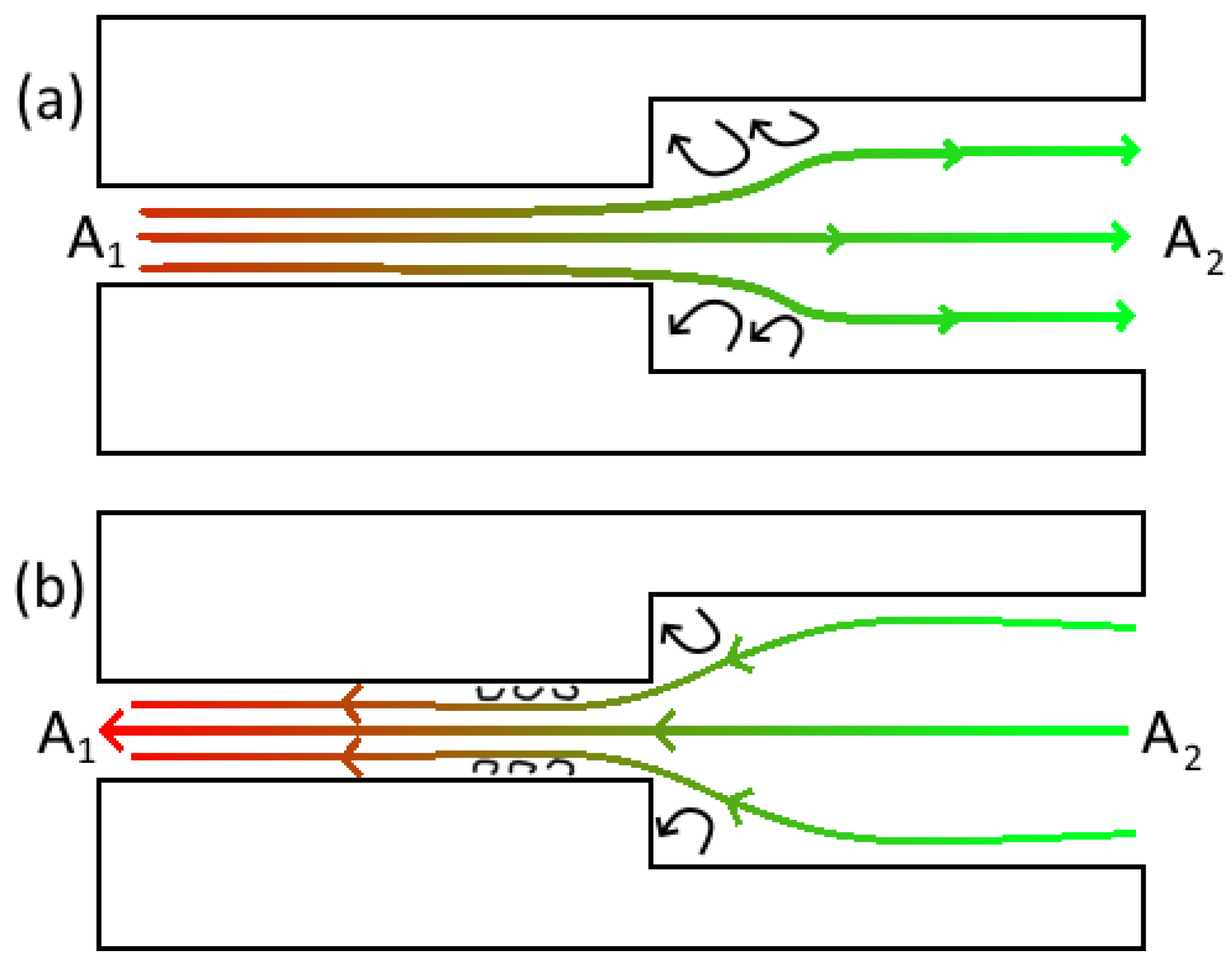
The present paper examines the numerical modeling of sound wave propagation in a pipe with an abrupt area change, as shown in Figure 1, using computational fluid dynamics (CFD). Iguchi [5] formulated a hypothesis in which oscillatory flow could be considered quasi-steady, allowing for the use of steady flow correlations for minor losses. In this hypothesis, the flow is assumed, at any point in time, to behave independently of its history, such that minor losses for flow in a given direction will correspond to the associated correlation for steady flow in that direction. Simplified steady-flow models for thermoacoustic minor losses have been described by Swift [6], while steady-flow heat transfer models have been also utilized [7]. Though the basic form of the thermoacoustic wave equation accounts for thermoviscous losses near pipe walls, it is not able, in itself, to account for turbulent motion or minor losses. The turbulent effects can be addressed to some degree by modifications to the viscous form function, which accounts for viscous losses as well as an adjusted thermal penetration depth [8]. Minor losses are usually represented by a pressure jump corresponding to upstream and downstream minor loss coefficients $K_{+}$ and $K_{-}$. DeltaEC, a thermoacoustic modeling software developed by Ward et al. [8], provides examples of lumped-element minor losses based on such upstream and downstream coefficients. Swift and Backhaus [9] described a high-performance thermoacoustic engine. Such devices are attractive for use with acoustic cryocoolers, due to their direct production of acoustic power and a lack of moving parts, which reduces maintenance needs. The design employed an acoustic jet pump, with minor losses modeled, and a regenerator of the engine based on steady flow correlations.

Hooper presented several empirical correlations for steady-flow minor loss coefficients [10]. Of particular note are the correlations for expansion and contraction of tubes with abrupt changes in diameter. At low Reynolds numbers, relatively simple correlations may be applied, being a function of area ratios and Reynolds numbers. At higher Reynolds numbers, the Moody friction factor is introduced. However, the steady-flow correlations are not designed for use with oscillatory flow.

Doller [11] performed experimental research in a set of geometries representing area changes at varying angles of tapering for both quarter- and half-wave acoustic resonators. By measuring both time-averaged pressure drop and energy dissipation, he derived experimental values for upstream and downstream minor loss coefficients. Both upstream and downstream minor loss coefficients obtained from the experiment showed agreement with steady flow predictions of Idelchik [12] for certain transitions but were noted to not have converged to an asymptotic value. In the 90-degree junction case, the asymptotic value of the upstream minor loss coefficient significantly exceeded the Idelchik correlation.

King and Smith [13] likewise analyzed minor losses in an experimental acoustic system with a tapered diffuser, examining the effects of displacement amplitude, Reynolds number, and taper angle. They found that minor losses decrease with Reynolds number and increase with displacement amplitude. Furthermore, depending on the displacement amplitude, minor losses may be either greater than or smaller than those predicted by steady flow correlations. Larger tapering angles were also observed to result in higher minor losses, but a description of the form of the trend was not given.

Ueda et al. [14] examined experimental correlations and compared them to a single minor loss coefficient for systems with air and high-pressure helium. They found the effect of different frequencies and impedances on minor loss coefficients at ambient temperature to be relatively weak. A correlation was also established that indicated tapering the abrupt area change produces a roughly linear progression between 15 and 90 degrees, decreasing to a minimum value at 15 degrees and below. Their methods displayed a good agreement between experimental values and what was predicted from correlations for an apparatus with a very large change in area, where the correlations are more accurate. However, experimental comparisons to values predicted for the minor loss coefficient at varying area ratios indicated significant departures from the correlations at several conditions.

Analysis of minor losses in experimental cryogenic systems is generally lacking. Regier [15] utilized a lumped element method to model a multiphase cryogenic helium system, with minor losses considered at junctions. However, these values were not determined in relation to any manner of correlation; rather, they were derived from experimental data for the real apparatus to correspond solely to the subject of study. Consequently, they are not generally applicable for broader analysis. Ding et al. [16] examined minor losses in 90- and 180-degree bends as a function of tube curvature for a thermoacoustic cooler; however, the operating fluid was high-pressure air at ambient temperatures, which may not be directly applicable to cryogenic fluids in particular.

Morris et al. [17] performed numerical simulations of acoustic minor losses in a pipe with abrupt area change for comparison with a set of experimental results. These losses were gauged by measuring the pressure drop across the area transition, outside the area spanned by vortices. They found that the standard time-averaged pressure drop correlation, based on steady flow, tends to underpredict pressure drop, and consequently overpredicts minor loss coefficients calculated from it.

Oosterhuis et al. [18] also performed numerical simulations of acoustic minor losses in an acoustic jet pump rather than a simple area-changing pipe. They noted that the commonly used model suggested by Backhaus and Swift [9] has significant quantitative disagreements with experimental data. Results confirmed the relationship of time-averaged dissipated power to the cube of oscillatory velocity amplitude; however, they found that the steady flow correlations only work for a limited range of ratios in fluid particle displacement versus jet pump length and considerably diverge outside of that range.

Yang et al. [19] produced a numerical simulation for a thermoacoustic engine, examining the formation of vortices in a short tube with an abrupt area transition. Results from computational fluid dynamics (CFD) were compared to DeltaEC, with a detected difference of up to 30%, where acoustic velocity and pressure in the CFD results were lower than in DeltaEC. The authors consider this to be an acceptable degree of error due to the effects accounted for by CFD, which are not included in DeltaEC.

Di Meglio and Massarotti [20] reviewed the current state of computational modeling in thermoacoustics. Relevant aspects of non-linear modeling that they cover include harmonics, turbulence, and mass streaming. For flow of sufficiently high amplitude, higher-order harmonics of the system’s fundamental frequency occur, which invalidate lower-order single-frequency assumptions commonly used in thermoacoustic approximations. Turbulence has a significant impact, potentially altering results by a factor of two in thermoacoustic applications [20]. They note that, in many cases, the k-ω SST performs the best for turbulence models in the Reynolds-Averaged Navier-Stokes (RANS) approach, but that there is no consensus on the best model to employ. Large eddy simulation is an alternative turbulence model but is less common due to its greater computational requirements. Mass streaming is a generally detrimental phenomenon, in which a net time-averaged mass flow occurs in a thermoacoustic system. One of its causes is a time-averaged pressure differential resulting from minor losses, while minor losses can also be used deliberately to counteract mass streaming.

Kurai et al. [21] modeled minor losses in a thermoacoustic refrigerator. A bended tube in the resonator and a T-junction were experimentally analyzed to determine their minor losses. Of some note is the finding that tube length has an effect, albeit a weak one, on the minor loss coefficient. While the data were not a perfect fit over the range analyzed, they were relatively close to linear in proportion to the velocity cubed, indicating a constant minor loss coefficient for a given geometry. A relatively consistent value is also reached at higher curvature ratios. In a T-junction, a similar dependence is also observed. However, results were not compared to correlations for steady flow or to analytical considerations.

The present study aims to produce correlations for a single time-averaged minor loss coefficient at a junction between tubes of different diameters from a set of parametric CFD simulations with cryogenic hydrogen. These correlations are based on the relevant characteristics of temperature, modified Reynolds number, pipe transition area ratio, and wave phasing (standing or traveling) in a pipe component with an abrupt area change. The cryogenic hydrogen is chosen as the fluid of interest in this study since it is a promising candidate to serve as a working fluid in novel cryocoolers [3] and as a renewable and clean fuel in the future economy [22,23,24]. The CFD approach is, nowadays, commonly used for modeling hydrogen systems [25,26], as it can provide detailed flow-field characteristics while reducing costs and safety concerns of conducting experiments.

2. Materials and Methods

2.1. Computational Fluid Dynamics Aspects

The simulations presented in this study are performed using the computational fluid dynamics (CFD) software Star-CCM+, version 15.04.008, which employs a finite-volume segregated compressible viscous solver with second-order space discretization and first-order implicit time stepping. The Reynolds-Averaged Navier-Stokes (RANS) approach is utilized with the governing continuity, momentum, and energy equations [27]:

$${\displaystyle \frac{\partial \rho }{\partial t}}+{\displaystyle \frac{\partial \left(\rho {\overline{u}}_j\right)}{\partial x_j}}=0,$$

(1)

$${\displaystyle \frac{\partial \left(\rho {\overline{u}}_i\right)}{\partial t}}+{\displaystyle \frac{\partial \left(\rho {\overline{u}}_i{\overline{u}}_j\right)}{\partial x_j}}=-{\displaystyle \frac{\partial p}{\partial x_i}}+{\displaystyle \frac{\partial }{\partial x_j}}\left[\mu \left({\displaystyle \frac{\partial {\overline{u}}_i}{\partial x_j}}+{\displaystyle \frac{\partial {\overline{u}}_j}{\partial x_i}}-{\displaystyle \frac{2}{3}}{\delta }_{ij}{\displaystyle \frac{\partial {\overline{u}}_k}{\partial x_k}}\right)-\rho \overline{{u^{\prime }}_i{u^{\prime }}_j}\right],$$

(2)

$${\displaystyle \frac{\partial \left(\rho E\right)}{\partial t}}+{\displaystyle \frac{\partial \left(\rho E{\overline{u}}_j\right)}{\partial x_j}}={\displaystyle \frac{\partial }{\partial x_j}}\left[-p{\overline{u}}_i{\delta }_{ij}+u_i\left\{\mu \left({\displaystyle \frac{\partial {\overline{u}}_i}{\partial x_j}}+{\displaystyle \frac{\partial {\overline{u}}_j}{\partial x_i}}-{\displaystyle \frac{2}{3}}{\delta }_{ij}{\displaystyle \frac{\partial {\overline{u}}_k}{\partial x_k}}\right)-\rho \overline{{u^{\prime }}_i{u^{\prime }}_j}\right\}\right]-{\displaystyle \frac{\partial q_j}{\partial x_j}},$$

(3)

where ${\overline{u}}_i$ are the Reynolds-averaged velocity components, $p$ is the pressure, $\rho$ is the fluid density, $\mu$ is the dynamic viscosity, $-\rho \overline{{u^{\prime }}_i{u^{\prime }}_j}$ is the turbulent stress tensor, $E$ is the total energy per unit mass, and $q_j$ are the heat fluxes.

In this study, the blended, two-layer realizable $k-\epsilon$ turbulence model is utilized [28,29]. This variation of the model is suited for both low and high wall y+ values and is significantly more accurate than the standard $k-\epsilon$ model in boundary layer flow and for modeling flow with jets, separation, and recirculation, which is crucial for adequately modeling acoustic minor losses. The Reynolds turbulent stress is formulated using the Boussinesq hypothesis:

$$-\rho \overline{{u^{\prime }}_i{u^{\prime }}_j}={\mu }_t\left({\displaystyle \frac{\partial u_i}{\partial x_j}}+{\displaystyle \frac{\partial u_j}{\partial x_i}}-{\displaystyle \frac{2}{3}}{\delta }_{ij}{\displaystyle \frac{\partial u_k}{\partial x_k}}\right)-{\displaystyle \frac{2}{3}}\rho E_k{\delta }_{ij},$$

(4)

with the viscosity of turbulent eddies, ${\mu }_t$, and the turbulent kinetic energy per unit mass, $E_k$. The governing equations of the $k-\epsilon$ model describe the turbulent kinetic energy $E_k$ and the turbulent dissipation rate $\epsilon$:

$${\displaystyle \frac{\partial \left(\rho E_k\right)}{\partial t}}+{\displaystyle \frac{\partial \left(\rho E_k{u}_j\right)}{\partial x_j}}={\displaystyle \frac{\partial }{\partial x_j}}\left[\left(\mu +{\displaystyle \frac{{\mu }_t}{{\sigma }_k}}\right){\displaystyle \frac{\partial E_k}{\partial x_j}}\right]+G_k-\rho \epsilon ,$$

(5)

$${\displaystyle \frac{\partial \left(\rho \epsilon \right)}{\partial t}}+{\displaystyle \frac{\partial \left(\rho \epsilon u_j\right)}{\partial x_j}}={\displaystyle \frac{\partial }{\partial x_j}}\left[\left(\mu +{\displaystyle \frac{{\mu }_t}{{\sigma }_{\epsilon }}}\right){\displaystyle \frac{\partial \epsilon }{\partial x_j}}\right]+\rho C_{\epsilon 1}S\epsilon -\rho C_{\epsilon 2}{\displaystyle \frac{{\epsilon }^2}{E_k+\sqrt{\nu \epsilon }}},$$

(6)

where $G_k$ is the production of turbulent kinetic energy by mean velocity gradients, $S=\sqrt{2 S_{ij}{S}_{ij}}$ is the scalar invariant of the strain rate tensor $S_{ij}={\displaystyle \frac{1}{2}}\left({\displaystyle \frac{\partial u_i}{\partial x_j}}+{\displaystyle \frac{\partial u_j}{\partial x_i}}\right)$, $\nu$ is the kinematic viscosity, $C_{\epsilon 1}$ and $C_{\epsilon 2}$ are the model coefficients, and σ_k and σ_ε are the turbulent Prandtl numbers for $E_k$ and $\epsilon$, respectively. The turbulent eddy viscosity, ${\mu }_t$, is defined by:

$${\mu }_t=\rho C_{\mu }{\displaystyle \frac{{E_k}^2}{\epsilon }},$$

(7)

where $C_{\mu }$ depends on the turbulence properties and mean flow [30].

Cryogenic parahydrogen gas was modeled by implementing property tables, generated using the open-source software CoolProp [31]. These tables included thermodynamic properties, as well as relevant transport properties as functions of pressure and temperature.

For computational efficiency, the numerical domain was modeled as a two-dimensional axisymmetric region near the pipe transition (Figure 2). Each straight tube section is 4 cm long, giving a total domain length of 8 cm. The left side of the domain is a narrow pipe with a fixed 2-mm radius. The right side is the wider pipe section with a radius ranging from 2.5 mm to 5 mm, depending on the area ratio for a given simulation. The upper and step wall boundaries are represented by no-slip, fixed-temperature walls, while the lower boundary delineates the axis of symmetry. Prism layers provide greater mesh refinement near the wall, while further away the domain consists of quadrilateral cells. Additional refinement is present at the transition zone between the tubes to better capture flow separation.

The left boundary is a velocity inlet, set to produce an oscillating velocity at a fixed frequency and amplitude. Its temperature has an oscillating value to match acoustic pressure fluctuation. The right-hand boundary differs depending on wave phasing. The standing wave boundary is very simple, being a pressure outlet at zero acoustic pressure (i.e., the outlet pressure is fixed to the mean pressure value). In the traveling wave case, the right-hand boundary is instead a velocity inlet, set to a velocity and temperature based on a pressure fluctuation in a sound wave propagating further downstream in a lossless duct of the same diameter.

The mesh displayed in Figure 2 showed significant robustness in sensitivity studies, producing little variation in relevant metrics at higher levels of coarseness. Dependences of the consumed acoustic power and RMS values of inlet acoustic pressure on the cell counts are given in Figure 3 for 30 K parahydrogen traveling- and standing-wave systems with area ratio 0.25 and inlet velocity amplitude 15 m/s. The final cell counts of grids used for parametric studies were between 11,166 and 14,202, depending on the area ratios. Additionally, time step sensitivity indicates fairly little change between different time steps once the time step is fine enough to avoid numerical instabilities. This provides confidence that numerical error is small in this configuration. At 30 K temperature, the selected time step, 5 × 10⁻⁵ s, represents 1/1000 of a cycle at 20 Hz oscillations and is slightly below the threshold where numerical instabilities are observed to occur, at a time step of 7 × 10⁻⁵ s. At higher velocities employed in 80 Kelvin simulations, which require faster flow to match Reynolds numbers, the time step is reduced to 1 × 10⁻⁵ s to preserve fidelity.

The relevant metric to evaluate acoustic losses is the acoustic power, obtained by integrating the acoustic power flux:

$$e_a=p^{\prime }\left(t\right)u^{\prime }\left(t\right),$$

(8)

over the cross-section of the tube, with time-dependent acoustic pressure $p\prime$ and acoustic velocity $u\prime$. The time-averaged acoustic power values are calculated over a single period at the inlet and outlet in a repeatable limit-cycle regime after a settling interval (usually about two cycles), and the acoustic power dissipated in the entire domain is found as the difference between the mean inlet and outlet power.

2.2. Thermoacoustic Model

To process useful data from CFD results, a distinction must be made between major losses (i.e., losses due to friction and thermal relaxation at the pipe walls) and minor losses near the tube transitions. The acoustic power dissipated in CFD simulations represents a combination of both effects. The identification of the major-loss portion is performed in this study by using a reduced-order thermoacoustic model. The minor loss in CFD is then determined by subtracting the major loss (computed with the thermoacoustic model) from the total acoustic power dissipation obtained in CFD.

The transfer function method such as that employed in DeltaEC [8] is utilized to describe variations of the amplitudes of acoustic pressure, $p_1$, and volumetric velocity, $U_1$, along the straight tube sections:

$$p_{1,out}=p_{1,in}\cos \left(k\Delta x\right)-{\displaystyle \frac{i\omega p_m}{\left(1-f_{\nu }\right)kA}}{U}_{1,in}\sin \left(k\Delta x\right),$$

(9)

$$U_{1,out}=U_{1,in}\cos \left(k\Delta x\right)-{\displaystyle \frac{i\left(1-f_{\nu }\right)kA}{\omega p_m}}{p}_{1,in}\sin \left(k\Delta x\right),$$

(10)

$$k={\displaystyle \frac{\omega }{a}}\sqrt{{\displaystyle \frac{1+\left(\gamma -1\right)f_{\kappa }}{1-f_{\nu }}}},$$

(11)

where $k$ is the wave number, $p_m$ is the mean pressure, $i$ is the imaginary unity, $a$ is the speed of sound, $f_{\nu }$ and $f_{\kappa }$ are the viscous and thermal form functions [6], $\omega$ is the angular frequency, $\gamma$ is the heat capacity ratio, $A$ is the duct area, and $\Delta x$ is the duct length. Depending on the viscous penetration depth, given by ${\mathit{\delta }}_{\nu }=\sqrt{2\nu /\omega }$, the onset of turbulence is determined, according to Swift [6], by either of the two following equations:

$$Re\cong 2000,{\displaystyle \frac{r_0}{{\delta }_{\nu }}}<2,$$

(12)

$$R{e}_{{\delta }_{\nu }}={\displaystyle \frac{Re}{r_0/{\delta }_{\nu }}}\cong 1000,{\displaystyle \frac{r_0}{{\delta }_{\nu }}}>2,$$

(13)

where $r_0$ is the pipe radius, $Re=\rho uD/\mu$ is the Reynolds number, defined by flow velocity $u$, pipe diameter $D$, and dynamic viscosity $\mu$, and $R{e}_{{\delta }_{\nu }}$ is a modification to the Reynolds number defined by Equation (13). The turbulent flow correction is a modification to the laminar viscous form function and the thermal penetration depth, depending on Reynolds number, penetration depth, viscous form function, and Moody friction factor [6].

The thermoacoustic model utilized in this study consists of four nodes, each having a determined volumetric velocity and pressure amplitudes. Two of the nodes are at the inlet and outlet boundaries, while the other two are on two sides of the pipe transition. As the thermoacoustic model is defined in the frequency domain, the volumetric velocity amplitude $U_1$ at the inlet is set to a fixed value, while the outlet is set to either zero acoustic pressure in the standing wave case or, in the traveling wave case:

$$p_1={\displaystyle \frac{\rho a{U}_1}{A_2}},$$

(14)

where $\rho$ is the mean density, $U_1$ is the volumetric acoustic velocity evaluated at the outlet, and $A_2$ is the cross-sectional area of the larger tube. At the area jump, the pressure amplitude difference is defined by Swift [6] for a certain single minor loss coefficient $K$ and the local volumetric velocity amplitude $U_1$:

$$\Delta p_1=-{\displaystyle \frac{4\rho }{3\pi A_1^2}}K\left|U_1\right|U_1.$$

(15)

The system of equations for the acoustic amplitudes at the inlet, outlet, and before and after the tube transition is then simply solved to produce the pressure and velocity amplitude outputs. The time-averaged acoustic power at the inlet and outlet gives power dissipation caused by both major and minor losses, with the minor loss power component being dependent on the minor loss coefficient value. The total dissipated power from the reduced-order model is then compared to the result of CFD simulations. The $K$ value in the reduced-order model is iteratively varied until the total dissipated powers from CFD and reduced-order model match; this produces the minor loss coefficient for given geometry and acoustic conditions.

3. Results and Discussion

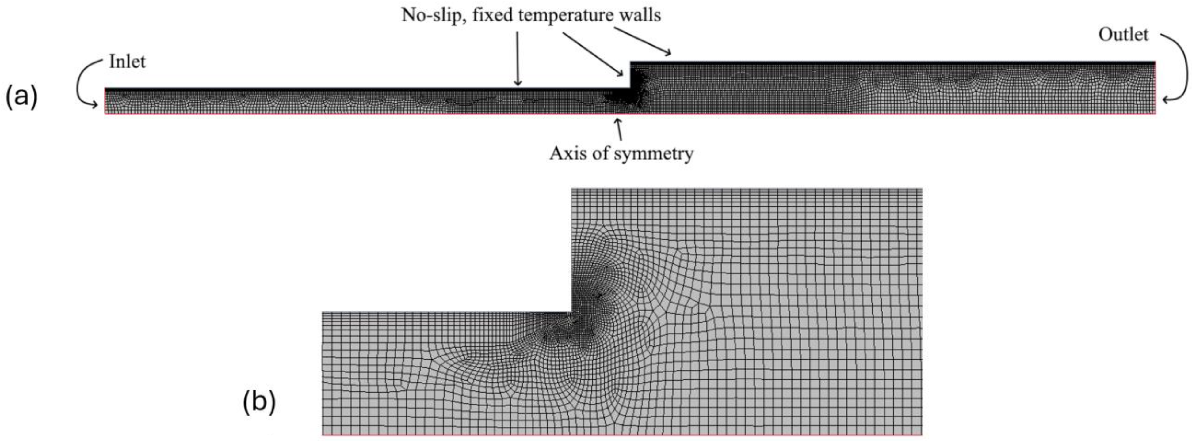
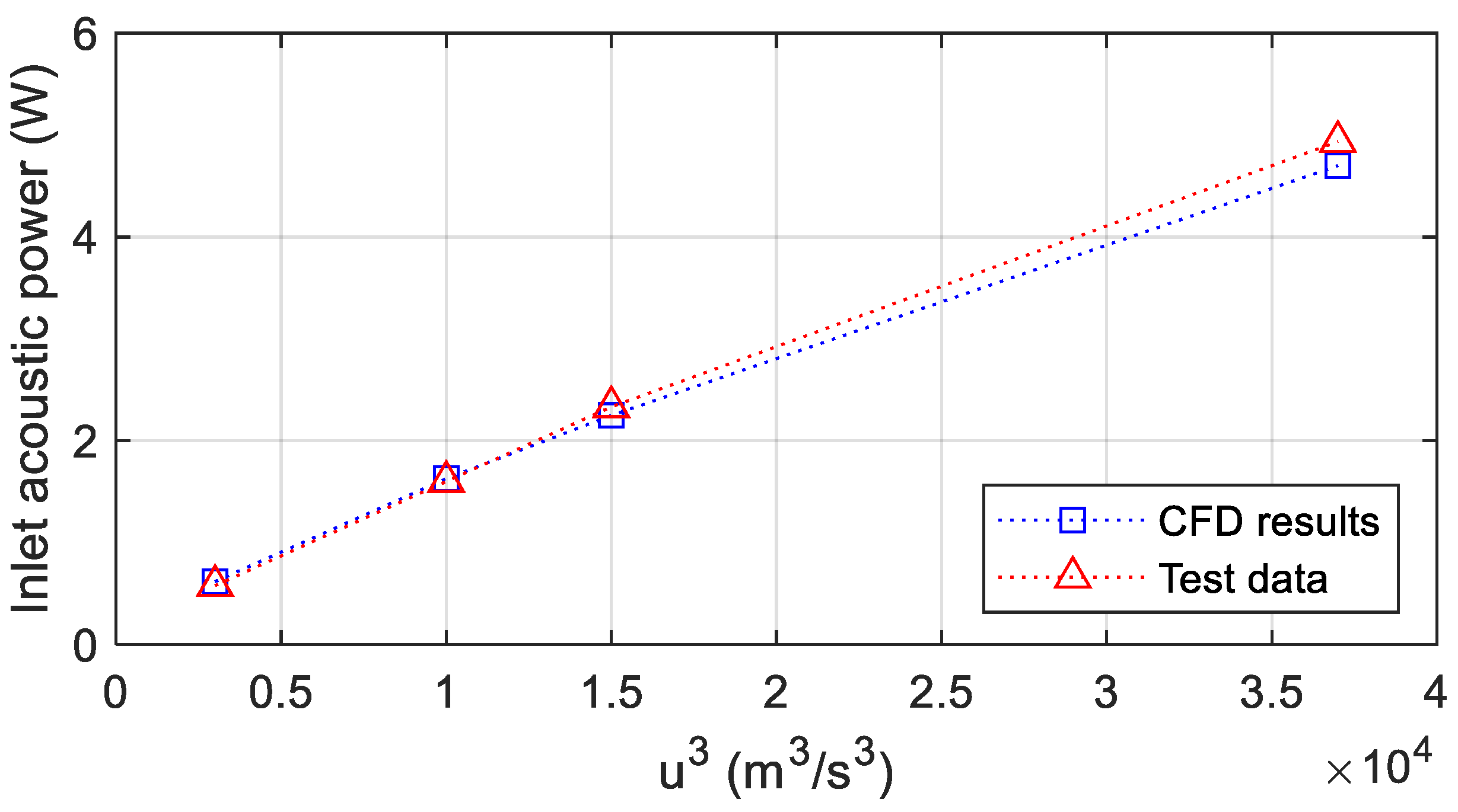
As no experimental data are available for acoustic minor losses in cryogenic hydrogen, test results from [14] obtained with atmospheric air were used for validation. The experimental setup included two tubes of different diameters with an acoustic driver on one side and a closed end on the other. CFD simulations have been run for that system, and a comparison between numerical and experimental inlet acoustic power is given in Figure 4. The agreement is deemed reasonable.

A series of parametric CFD simulations with cryogenic hydrogen has been performed in this study. The modeled fluid is parahydrogen at 30 and 80 K. Due to the differences in density and viscosity between the two temperatures, the modified Reynolds number at 80 K is much lower than at 30 K for the same velocity amplitudes. Consequently, to generate an overlapping range of Re values, the 30 K simulation is run at the inlet velocity amplitudes of 3, 5, 9, 15, and 25 m/s, while the 80 K simulation is run at 6.2, 9, 15, 25, 40, and 70 m/s. Three area ratios, defined by the ratio of the smaller to the greater area, are selected, being 0.16, 0.25, and 0.64, corresponding to a narrow tube radius of 2 mm and wide tube radii of 2.5, 4, and 5 mm, respectively. Additionally, each simulation is run with both standing and traveling wave phasings. The oscillation frequency is fixed at 20 Hz for all cases.

Post-processing involves extracting data of unsteady acoustic power flow, determined by integrating acoustic power flux over the inlet and outlet. The time-averaged acoustic powers at the inlet and outlet are calculated by numerically integrating them over a single period of in repeatable-cycle regime at each inlet velocity amplitude value. This power is compared with a reduced-order model using an adjustable minor loss coefficient $K$. 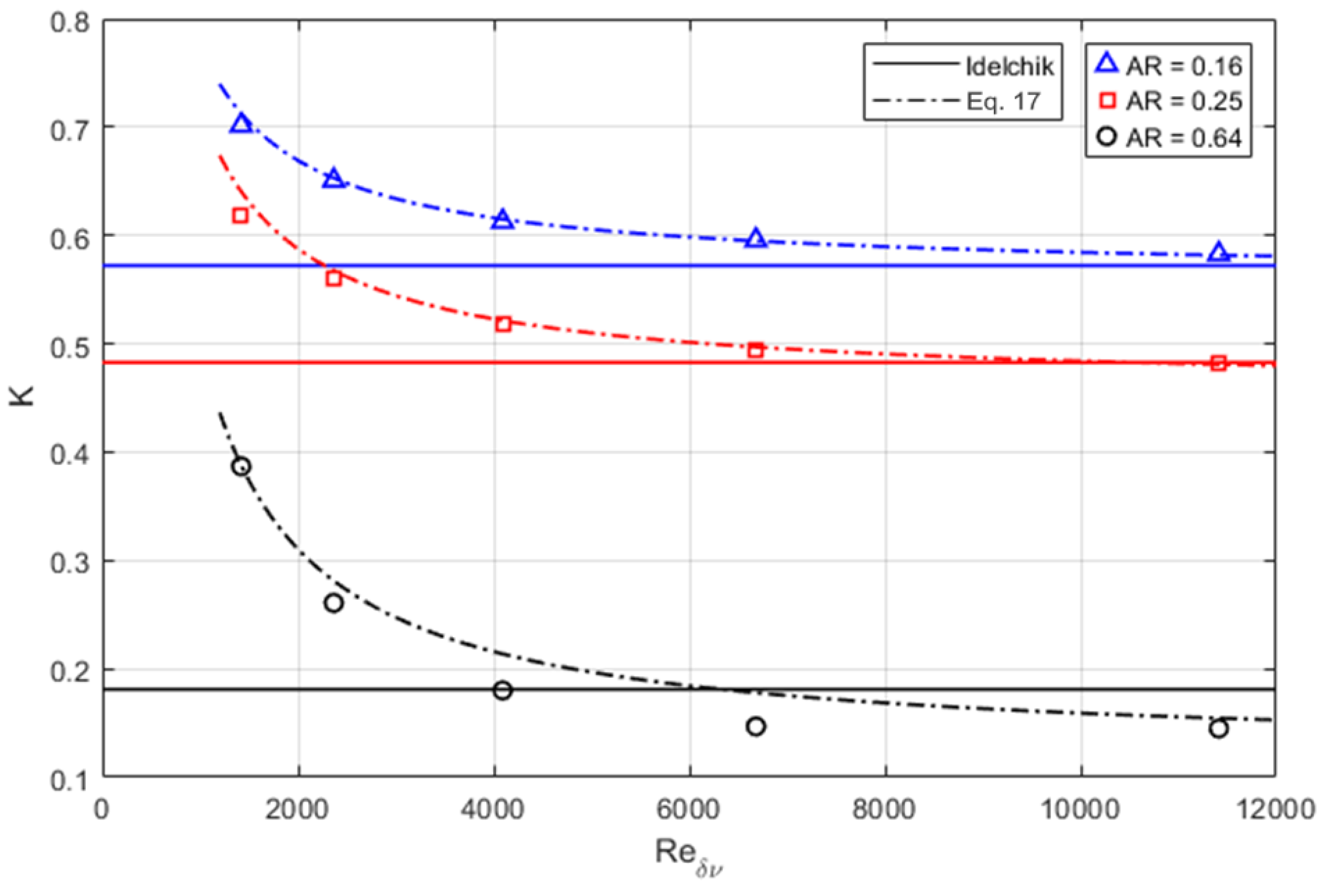The results for the minor loss coefficient obtained this way are reported in Figure 5.

The values of minor loss coefficients to which the CFD data converge at high Reynolds number for different area ratios are relatively close to the values predicted for the mean coefficient by the empirical correlation of Idelchik [12]:

$$K={\displaystyle \frac{1}{2}}{\left(1-{\displaystyle \frac{A_1}{A_2}}\right)}^2+{\displaystyle \frac{1}{4}}{\left(1-{\displaystyle \frac{A_1}{A_2}}\right)}^{0.75},$$

(16)

where $A_1$ and $A_2$ are the cross-section areas of narrower and wider tube sections. A comparison of CFD minor loss coefficients against the constant values predicted by Equation (16) for given area ratios indicates that loss coefficients significantly differ at lower Reynolds numbers (Figure 5). This result is consistent for all area ratios, temperatures, and two wave phasings. Traveling and standing waves display some difference for $K$, with standing waves having a lower minor loss coefficient. Furthermore, the factor by which minor loss coefficients deviates from Idelchik correlation depends on area ratio, with greater area ratio (i.e., a smaller difference in area) showing greater deviation. Thus, the numerically evaluated minor loss coefficients display an inverse dependence on Reynolds number, which also scales proportionally to some power of area ratio.

A simplified correlation has been derived based on the average of the curves in the data, as shown in Figure 6. It can be assumed, in a similar manner to the correlations provided by Hooper [10], that the correction factor will be in the form of a constant plus a second constant divided by Reynolds number. Additionally, it may be altered by a factor based on the area ratio to account for observed effects. The modified minor loss value, accounting for Reynolds number and area ratio effects, is proposed in the following form for the studied range of parameters:

$$K_{modified}=\left(1.2+{\displaystyle \frac{256+4480A{R}^2}{R{e}_{{\delta }_{\nu }}}}\right)K-0.125\sqrt{1-A{R}^2},$$

(17)

where $K$ is given by Equation (16), $R{e}_{{\delta }_{\nu }}$ is defined by Equation (13), and $AR=A_1/A_2$ is the area ratio.

The comparisons between correlations from Equation (17) and Idelchik, and the CFD results, averaged between temperatures, wave phasing, and close Reynolds numbers at each area ratio, are included in Figure 6. The deviation between the proposed correlation (Equation (17)) and averaged CFD results is smaller than scatter of CFD datapoints (Figure 5).

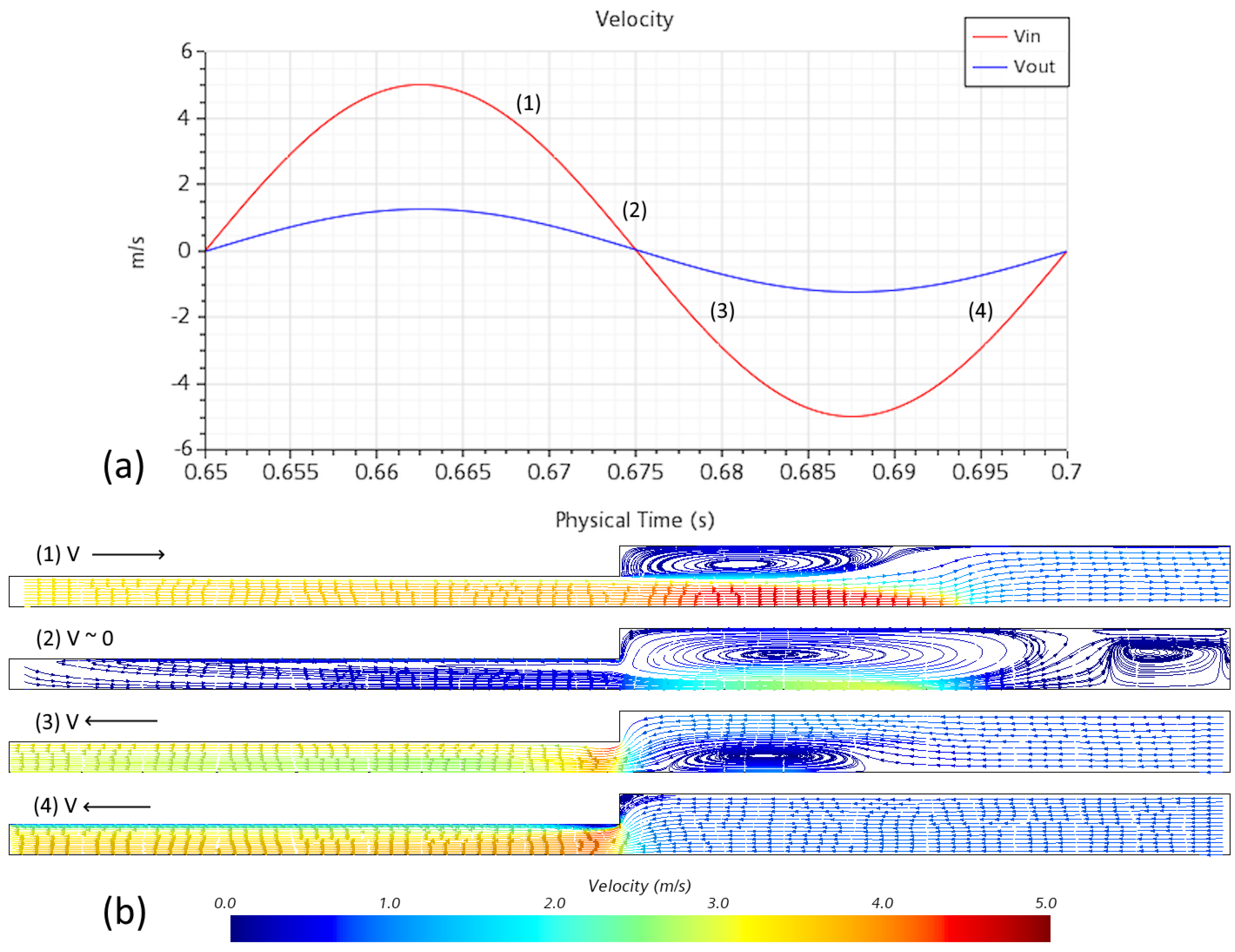
To provide insight on evolutions of flow-field variables during an acoustic cycle, time-dependent variations of some inlet/outlet flow properties and velocity streamlines are shown in Figure 7, Figure 8 and Figure 9. Velocity streamlines in Figure 7b are given at different instances, marked in Figure 7a, in a cycle for a 30 K simulation with 5 m/s inlet velocity amplitude for traveling wave phasing. During the blowing part of the cycle at instance (1) in Figure 7a (with positive inlet velocity), a jet forms in the wider tube segment after the step, while a recirculation zone is visible outside this jet behind the step. As the velocity decreases to roughly zero at the midpoint of the cycle at instance (2), the jet compresses towards the symmetry axis, while the recirculation zone expands. As flow reverses in the suction phase at instance (3), the recirculation zone moves towards to the tube axis, where it eventually disappears. As reverse flow fully develops (in the leftward direction), smaller recirculation zones are formed on both sides of the step at instance (4). The asymmetry in the formation of vortices will result in different losses during the blowing and suction stages of an acoustic cycle.

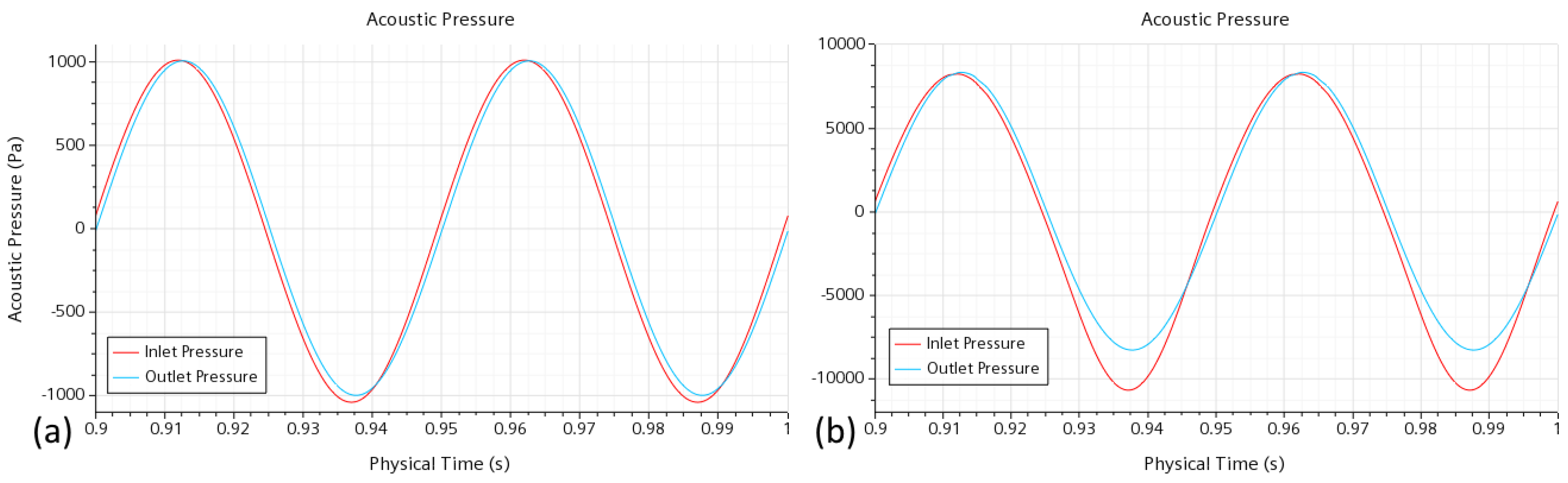
The acoustic pressure (difference between instantaneous and mean pressure) and acoustic power variations at the inlet and outlet are illustrated at two conditions (high and low inlet velocity amplitudes) in Figure 8 and Figure 9 for traveling wave oscillations. Stronger differences between the inlet and outlet properties are observed at large amplitudes in the second (suction) part of a cycle. 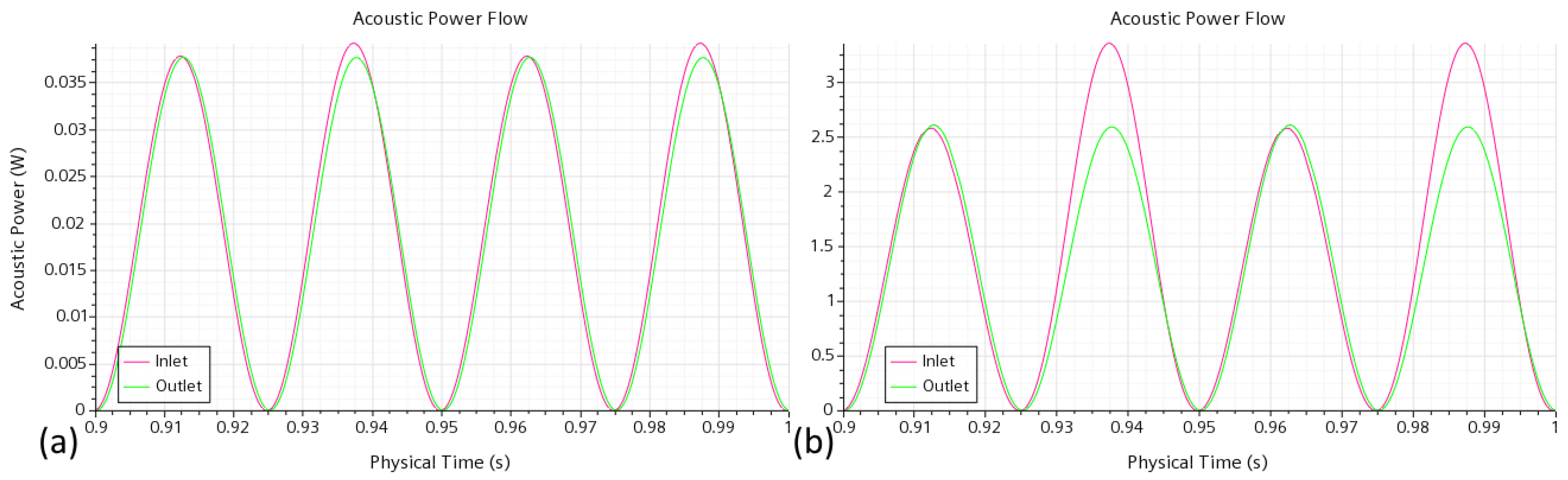The acoustic pressure troughs are significantly lower than peaks (Figure 8b), representing a deviation from sinusoidal behavior, which will also lead to a time-averaged pressure drop between the inlet and outlet. In the acoustic power graphs (Figure 9), two distinct intervals are also observed in the blowing and suction portions of the cycle. The asymmetry is also visible at low amplitudes (Figure 9a) but becomes highly magnified at greater amplitudes (Figure 9b). This behavior is associated with a smaller amount of total power exiting the system at the inlet in the suction half of a cycle (with the leftward flow direction), resulting in the net acoustic power flow entering the considered domain.

4. Conclusions

A CFD model is constructed to examine acoustic minor losses at an abrupt area change within a pipe for different temperatures and wave phasings in cryogenic hydrogen. The minor loss coefficient values are compared to the commonly used steady-flow correlation, and a correction factor for acoustic minor losses, accounting for viscous effects, is obtained based on numerical results. Specifically, an increase in the minor loss coefficient is found and quantified at lower Reynolds numbers. The obtained correlation describes the CFD results reasonably well in the studied range of temperatures and acoustic phases. As the area ratio approaches one, the minor loss coefficient will approach zero, but additional validation of this correlation may be necessary to assess its accuracy at very high and very low area ratios. The proposed correlation provides more accurate estimates for minor losses in cryogenic thermoacoustic systems, which can improve the accuracy of models for thermoacoustic cryocoolers and Taconis oscillations, especially in practically important high-amplitude regimes where the effect of minor losses can become prevalent.

Future research directions can include studying other geometries of relevance to cryogenics, such as open tube ends and tapered transitions between pipes. Quantifying nonlinear effects, such as the generation of higher harmonics mass streaming, will be also important for high-power thermoacoustic devices. Investigating multi-phase acoustic phenomena is another worthy, but much more computationally challenging, task.