
Computational Modeling of High-Speed Flow of Two-Phase Hydrogen through a Tube with Abrupt Expansion


Abstract
1. Introduction
2. Computational Modeling Aspects
3. Computational Setup
4. Results
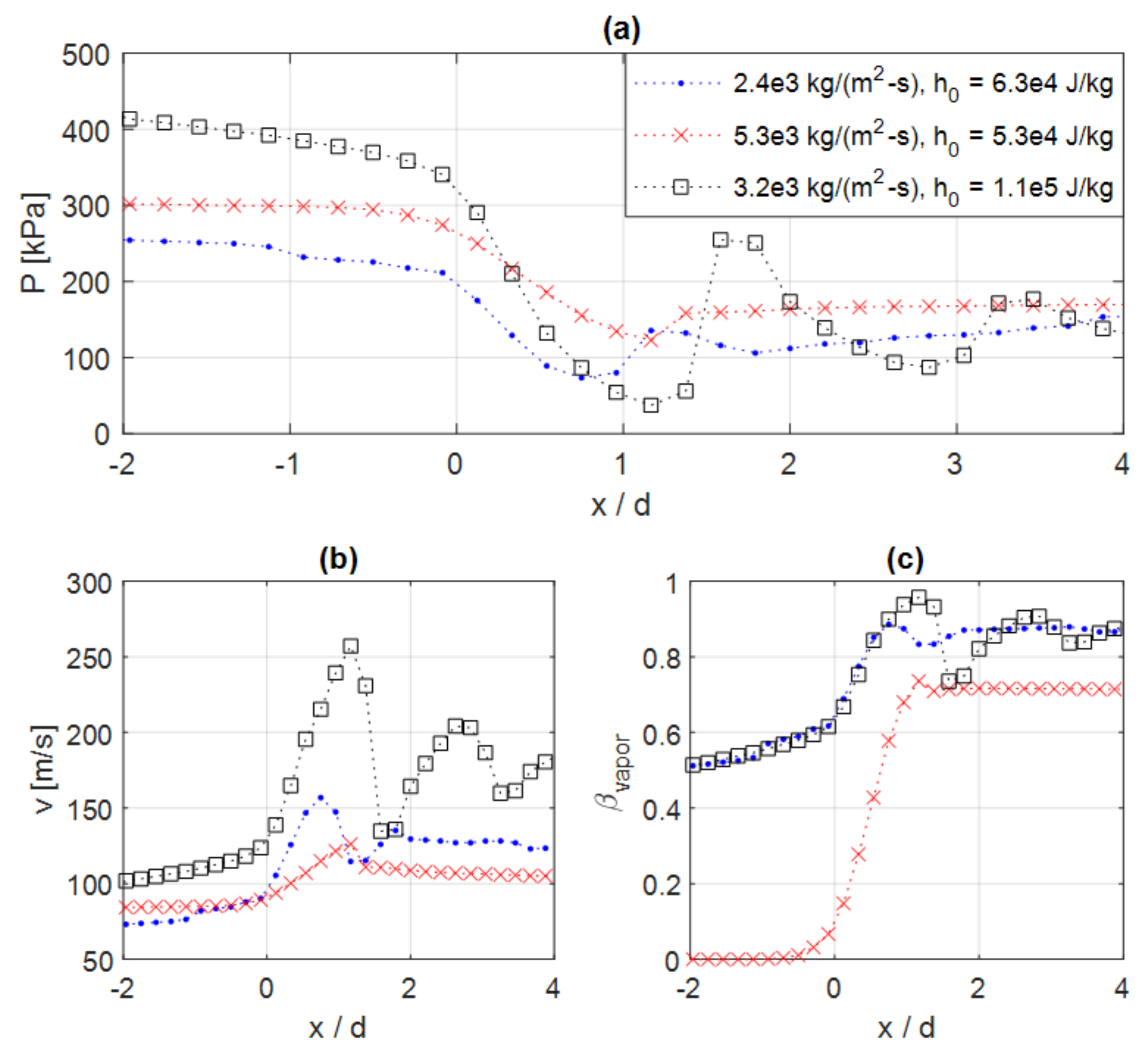
4.1. Verification and Calibration Study (Series #1)
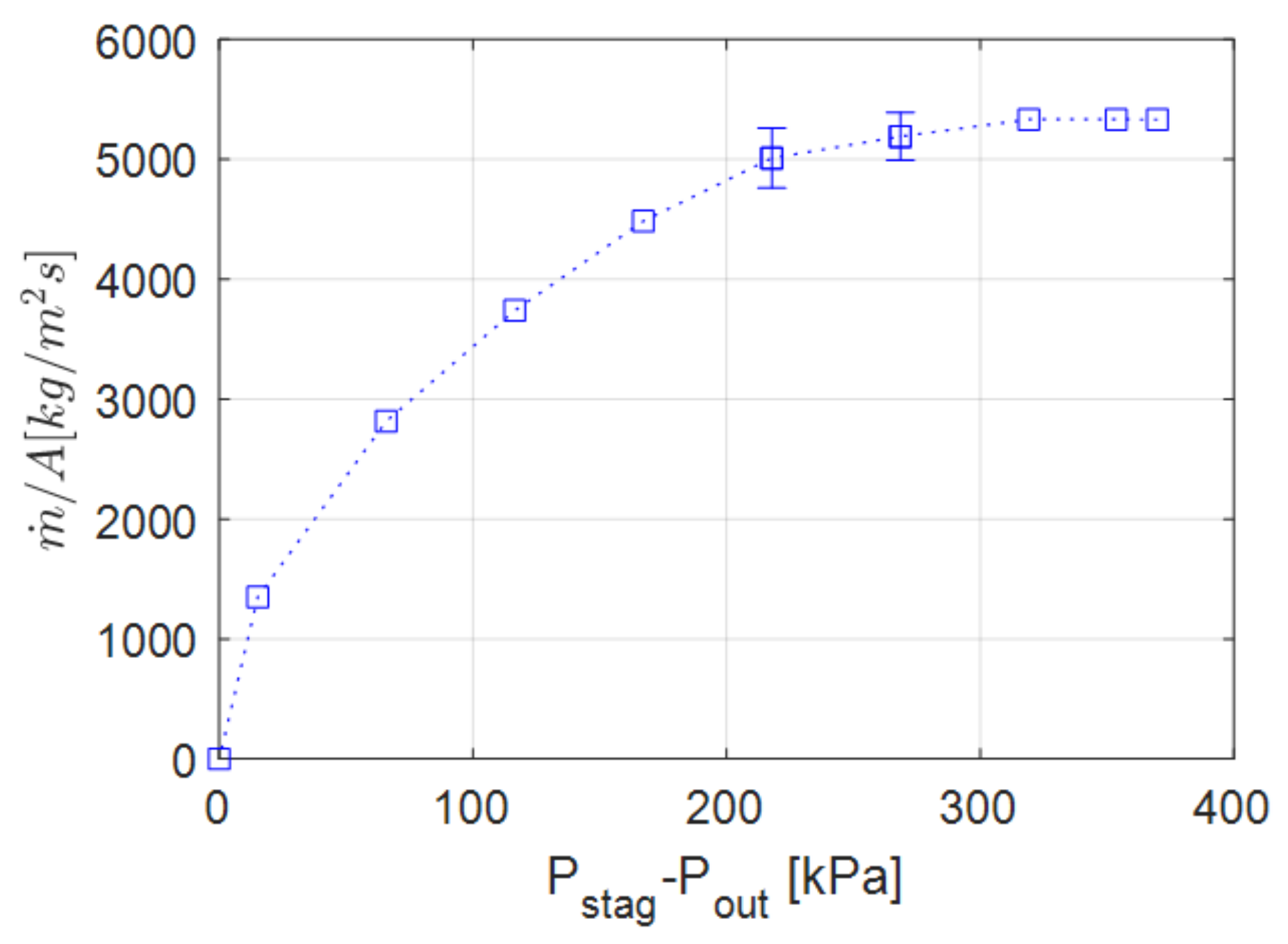
4.2. Variable Outlet Pressure Study (Series #2)
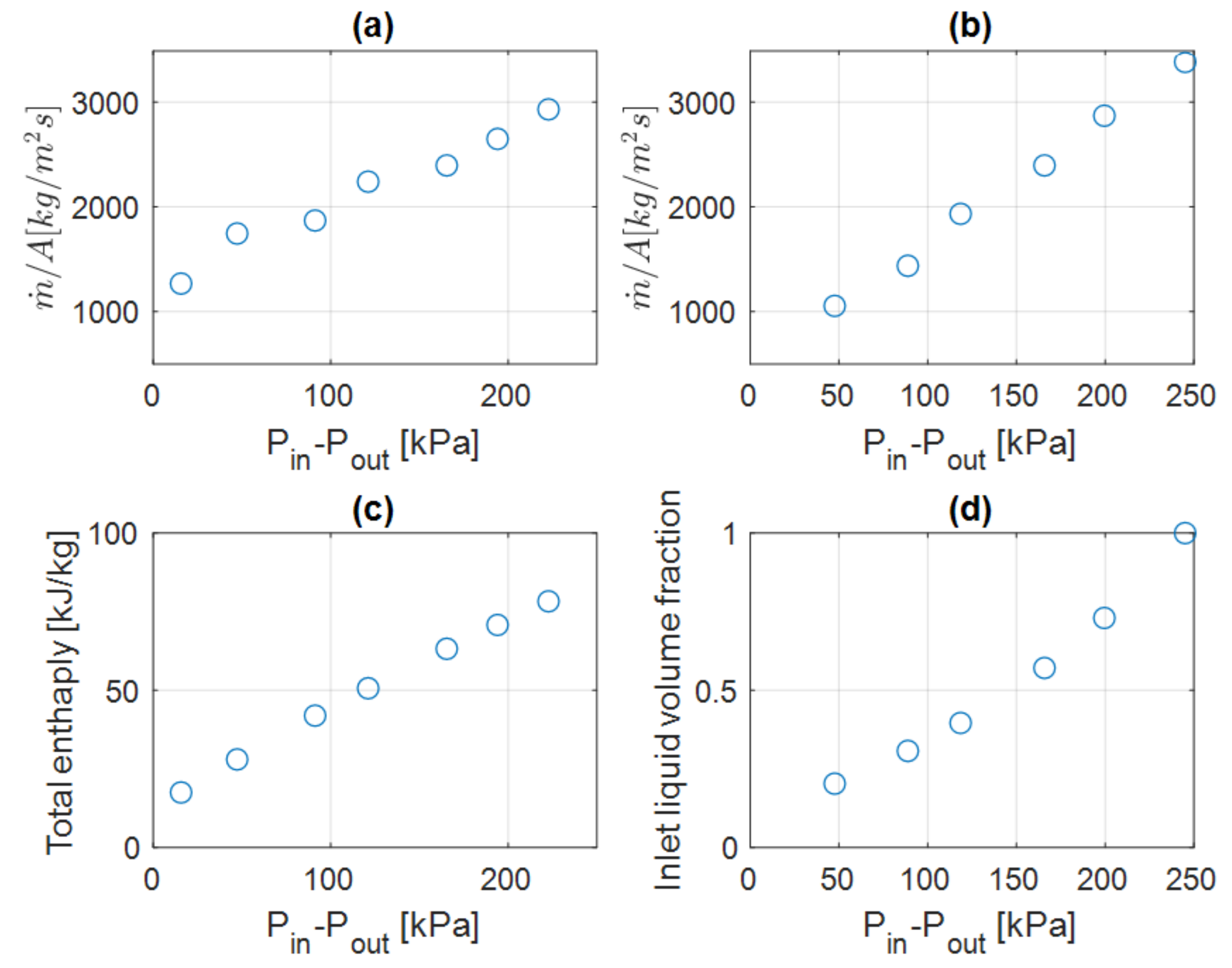
4.3. Variable Inlet Pressure Studies (Series #3 and #4)
5. Conclusions
Funding
Data Availability Statement
Acknowledgments
Conflicts of Interest
References
- Matveev, K.I.; Leachman, J.W. The effect of liquid hydrogen tank size on self-pressurization and constant-pressure venting. Hydrogen 2023, 4, 444–455. [Google Scholar] [CrossRef]
- Stolten, D.; Emonts, B. Hydrogen Science and Engineering: Materials, Processes, Systems and Technology; Wiley: Weinheim, Germany, 2016. [Google Scholar]
- Matveev, K.I.; Leachman, J.W. Modeling of liquid hydrogen tank cooled with para-orthohydrogen conversion. Hydrogen 2023, 4, 146–153. [Google Scholar] [CrossRef]
- Kartuzova, O.; Kassemi, M. Self-pressurization and spray cooling simulations of the multipurpose hydrogen test bed (MHTB) ground-based experiment. In Proceedings of the AIAA/ASME/SAE/ASEE Joint Propulsion Conference, Cleveland, OH, USA, 28–30 July 2014. [Google Scholar]
- Brennan, J.A.; Edmonds, D.K.; Smith, R.V. Two-Phase (Liquid-Vapor), Mass-Limiting Flow with Hydrogen and Nitrogen; Technical Note 359; National Bureau of Standards: Boulder, CO, USA, 1968. [Google Scholar]
- Smith, R.V.; Randall, K.R.; Epp, R. Critical Two-Phase Flow for Cryogenic Fluids; NBS Technical Note 633; National Bureau of Standards: Washington, DC, USA, 1973. [Google Scholar]
- Simoneau, R.J.; Hendricks, R.C. Two-Phase Choked Flow of Cryogenic Fluids in Converging-Diverging Nozzles; NASA Technical Paper 1484; Lewis Research Center: Cleveland, OH, USA, 1979.
- Kieffer, S.W. Sound speed in liquid-gas mixtures: Water-air and water-steam. J. Geophys. Res. 1977, 82, 2895–2904. [Google Scholar] [CrossRef]
- Henry, R.E.; Fauske, H.K. The two-phase critical flow of one-component mixtures in nozzles, orifices, and short tubes. J. Heat Transf. 1971, 93, 179–187. [Google Scholar]
- Gopalakrishnan, S.; Schmidt, D.P. A computational study of flashing flow in fuel injector nozzles. SAE Int. J. Engines 2009, 1, 160–170. [Google Scholar] [CrossRef]
- Battistoni, M.; Som, S.; Longman, D.E. Comparison of Mixture and Multifluid Models for In-Nozzle Cavitation Prediction. J. Eng. Gas Turbines Power 2014, 136, 061506. [Google Scholar] [CrossRef]
- Lee, W.H. A Pressure Iteration Scheme for Two-Phase Flow Modeling; Technical Report LA-UR 79-975; Los Alamos Scientific Laboratory: Los Alamos, NM, USA, 1979.
- Bilicki, Z.; Kestin, J. Physical aspects of the relaxation model in two-phase flow. Proc. R. Soc. Lond. A 1990, 428, 379–397. [Google Scholar]
- Downar-Zapolski, P.; Bilicki, Z.; Bolle, L.; Franco, J. The non-equilibrium relaxation model for one-dimensional flashing liquid flow. Int. J. Multiph. Flow 1996, 22, 473–483. [Google Scholar]
- Reocreux, M. Contribution a L’etude des Debits Critiques en Ecoulement Diphasique Eauvapeur. Ph.D. Thesis, Universit Scientifique et Medicale de Grenoble, La Tronche, France, 1974. [Google Scholar]
- Banaszkiewicz, M.; Kardas, D. Numerical calculations of the Moby Dick experiment by means of unsteady relaxation model. J. Theor. Appl. Mech. 1997, 35, 211–232. [Google Scholar]
- Schmidt, D.P.; Gopalakrishnan, S.; Jasak, H. Multi-dimensional simulation of thermal non-equilibrium channel flow. Int. J. Multiph. Flow 2010, 36, 284–292. [Google Scholar] [CrossRef]
- Travis, J.R.; Picconi Koch, D.; Breitung, W. A homogeneous non-equilibrium two-phase critical flow model. Int. J. Hydrog. Energy 2012, 37, 17373–17379. [Google Scholar] [CrossRef]
- Venetsanos, A.G. Homogeneous non-equilibrium two-phase critical flow model. Int. J. Hydrog. Energy 2018, 43, 22715–22726. [Google Scholar] [CrossRef]
- Wilhelmsen, O.; Aasen, A. Choked liquid flow in nozzles: Crossover from heterogeneous to homogeneous cavitation and insensitivity to depressurization rate. Chem. Eng. Sci. 2022, 248, 117176. [Google Scholar] [CrossRef]
- Bellur, K.; Medici, E.F.; Hermanson, J.C.; Choi, C.K.; Allen, J.S. Modeling liquid-vapor phase change experiments: Cryogenic hydrogen and methane. Colloids Surf. A Physicochem. Eng. Asp. 2023, 675, 131932. [Google Scholar] [CrossRef]
- Ferziger, J.H.; Peric, M. Computational Methods for Fluid Dynamics; Springer: Berlin, Germany, 1999. [Google Scholar]
- Rodi, W. Experience with two-layer models combining the k-ɛ model with a one-equation model near the wall. In Proceedings of the 29th Aerospace Sciences Meeting, Reno, NV, USA, 7–10 January 1991. [Google Scholar]
- Mulvany, N.; Tu, J.Y.; Chen, L.; Anderson, B. Assessment of two-equation modeling for high Reynolds number hydrofoil flows. Int. J. Numer. Meth. Fluids 2004, 45, 275–299. [Google Scholar] [CrossRef]
- Hirt, C.W.; Nichols, B.D. Volume of fluid (VOF) methods for the dynamics of free boundaries. J. Comput. Phys. 1981, 39, 201–225. [Google Scholar] [CrossRef]
- Wheeler, M.P.; Matveev, K.I.; Xing, T. Validation study of compact planing hulls at pre-planing speeds. In Proceedings of the 5th Joint US-European Fluids Engineering Summer Conference, Montreal, QC, Canada, 15–18 July 2018. [Google Scholar]
- Matveev, K.I.; Wheeler, M.P.; Xing, T. Numerical simulation of air ventilation and its suppression on inclined surface-piercing hydrofoils. Ocean Eng. 2019, 175, 251–261. [Google Scholar]
- STAR-CCM+ Manual. 2023. Available online: https://mdx.plm.automation.siemens.com/star-ccm-plus (accessed on 15 December 2023).
- Bell, I.H.; Wronski, J.; Quoilin, S.; Lemort, V. Pure and pseudo-pure fluid thermophysical property evaluation and the open-source thermophysical property library CoolProp. Ind. Eng. Chem. Res. 2014, 53, 2498–2508. [Google Scholar] [CrossRef] [PubMed]
- Leachman, J.W.; Jacobsen, R.T.; Penoncello, S.G.; Lemmon, E.W. Fundamental equations of state for parahydrogen, normal hydrogen, and orthohydrogen. J. Phys. Chem. Ref. Data 2009, 38, 721–748. [Google Scholar] [CrossRef]
- Roache, P.J. Verification and Validation in Computational Science and Engineering; Hermosa Publishers: Albuquerque, NM, USA, 1998. [Google Scholar]


| Simulation Series | Inlet Boundary Conditions | Outlet Boundary |
|---|---|---|
| Series #1 Calibration study for three test conditions = 5.33 × 10³ kg/(s·m2), = 5.27 × 10⁴ kJ/kg; = 2.40 × 10³ kg/(s·m2), = 6.34 × 10⁴ kJ/kg; = 3.23 × 10³ kg/(s·m2), = 1.09 × 10⁵ kJ/kg | Mass flow inlet: (i) Mass flow rate is assigned an experimental value (ii) Temperature is saturated for two-phase flow (b,c) or selected to keep the given total enthalpy for the inlet subcooled liquid state (a): = 27.0 K for two-phase flow or to be one for subcooled liquid: = 0.623 | Pressure outlet: = 168 kPa = 116 kPa = 135 kPa |
| Series #2 Variable outlet pressure study | Stagnation inlet: = 1 | Pressure outlet: is varied between 152 kPa and 522 kPa |
| Series #3 Variable inlet pressure study with constant inlet liquid volume fraction 0.571 | Pressure inlet: is varied between 131 kPa and 338 kPa (ii) Temperature is saturated = 0.571 | Pressure outlet: = 116 kPa |
| Series #4 Variable inlet pressure study with constant inlet total enthalpy 6.3 × 10⁴ J/kg | Pressure inlet: is varied between 163 kPa and 361 kPa (ii) Temperature is saturated (iii) Liquid volume fraction is selected to maintain given total enthalpy | Pressure outlet: = 116 kPa |
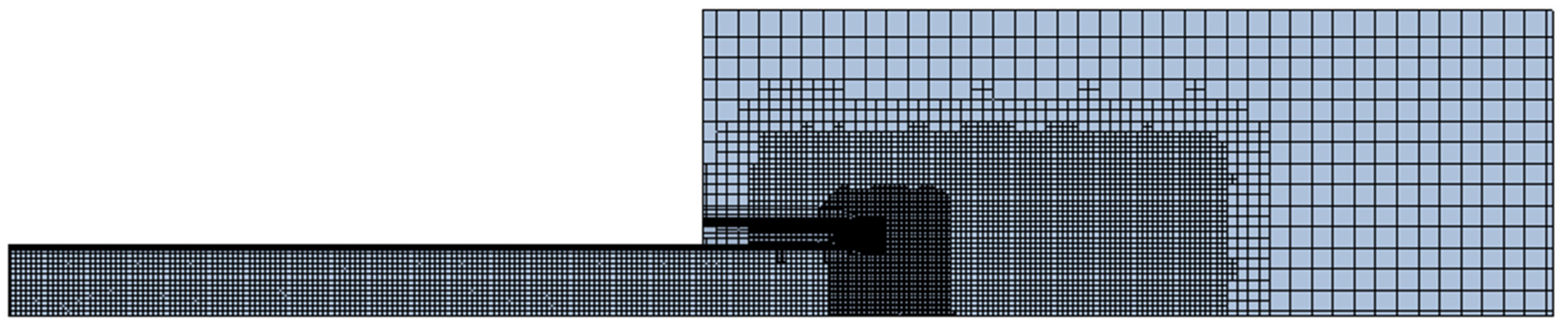
| Mesh | Cell Count | Cell Size near Tube Exit | Tube Exit Pressure |
|---|---|---|---|
| Coarse | 8999 | 0.62 mm | 182.8 kPa |
| Medium | 24,540 | 0.31 mm | 213.4 kPa |
| Fine | 117,914 | 0.16 mm | 220.1 kPa |
Disclaimer/Publisher’s Note: The statements, opinions and data contained in all publications are solely those of the individual author(s) and contributor(s) and not of MDPI and/or the editor(s). MDPI and/or the editor(s) disclaim responsibility for any injury to people or property resulting from any ideas, methods, instructions or products referred to in the content. |
© 2024 by the author. Licensee MDPI, Basel, Switzerland. This article is an open access article distributed under the terms and conditions of the Creative Commons Attribution (CC BY) license (https://creativecommons.org/licenses/by/4.0/).
Share and Cite
Matveev, K.I. Computational Modeling of High-Speed Flow of Two-Phase Hydrogen through a Tube with Abrupt Expansion. Hydrogen 2024, 5, 14-28. https://doi.org/10.3390/hydrogen5010002
Matveev KI. Computational Modeling of High-Speed Flow of Two-Phase Hydrogen through a Tube with Abrupt Expansion. Hydrogen. 2024; 5(1):14-28. https://doi.org/10.3390/hydrogen5010002
Chicago/Turabian StyleMatveev, Konstantin I. 2024. "Computational Modeling of High-Speed Flow of Two-Phase Hydrogen through a Tube with Abrupt Expansion" Hydrogen 5, no. 1: 14-28. https://doi.org/10.3390/hydrogen5010002
APA StyleMatveev, K. I. (2024). Computational Modeling of High-Speed Flow of Two-Phase Hydrogen through a Tube with Abrupt Expansion. Hydrogen, 5(1), 14-28. https://doi.org/10.3390/hydrogen5010002