Using Biodiversity Indices Effectively: Considerations for Forest Management

Abstract

Since biodiversity is a multifaceted aspect of natural systems, several indices have been suggested to measure it. In this paper, we examined a number of well-known diversity indexes to see whether some performed better than others when applied to forest data. In order to reach this goal, we used data on basic forest variables (such as the diameters, heights, and volumes of trees) from forest plots to see if common diversity indices lead to the same conclusions about changes in biodiversity in a pairwise comparison (i.e., comparing the same region at two different times or two different regions at the same time). Out of a collection of 17 diversity indices, 8 of them exhibited robustness, indicating their constant ability to demonstrate either an increase or decrease in biodiversity over pairwise comparisons. However, it is important to note that the remaining seven diversity indices may yield inconsistent or inconclusive results, but only with regard to forest data, highlighting the complexity and nuances of measuring biodiversity with different sorts of data. In this review article, all 17 indices are presented, allowing the reader to choose which ones are most applicable to their particular dataset (genetic, econometric, sociometric, etc.).

1. Introduction

Ecosystem services refer to the various benefits that ecosystems provide to enhance human well-being, both directly and indirectly. The maintenance and balance of ecosystem services provided by forests necessitate comprehensive assessment and evaluation across various spatial and temporal scales. Studies by [1,2,3] show that forest management decisions and strategies have implications for the provision of ecosystem services. The Millennium Ecosystem Assessment (MEA) identified four categories of ecosystem services: provisioning services (such as water, food production, carbon sequestration, and regulating services); cultural services (such as spiritual, historical, and social values); and supporting services (such as plant production and nutrient cycling). Biodiversity can fulfill three distinct functions in relation to ecosystem services: regulating ecosystem processes, serving as a final ecosystem service, or functioning as an asset [4]. Regulating ecosystem processes refers to the role of biodiversity in maintaining the balance and functioning of ecosystems, such as pollination by bees or natural pest control. Being a final ecosystem service means that humans can directly benefit from or value biodiversity itself, such as via leisure pursuits like birdwatching or ecotourism. Additionally, biodiversity can also function as an asset by providing opportunities for economic development and innovation, such as the discovery of new medicines from plant species.

The need to enhance monetary and socio-cultural valuation approaches to biodiversity with a scientific understanding of ecosystem functioning has led to the development of various biodiversity indices [5]. These indices aim to quantify and measure the state of biodiversity in a given area, providing valuable information for conservation efforts and policymaking. By incorporating scientific knowledge into valuation approaches, these indices help ensure that the true value of biodiversity is recognized and taken into account in decision-making processes.

Furthermore, they also contribute to our understanding of the intricate relationships between different species and their roles in maintaining ecosystem health and resilience. Biodiversity indicesare developedto describe species richness and distribution in various ways [6]. These indices provide a quantitative measure of the number and abundance of species in a given area, allowing for comparisons across different ecosystems. Additionally, they can help identify areas of high biodiversity importance and prioritize conservation efforts accordingly.

Many biodiversity indices have been suggested. Each biodiversity index weighs richness (number of categories, types, species, or classes) and distribution (number of observations per category, type, species, or class) differently [7]. By assigning different weights to richness and distribution, these indices capture the importance of both factors in determining overall biodiversity. This approach acknowledges that biodiversity is not solely determined by the number of different categories present but also by the distribution of observations within those categories. In this context, an area with a high number of species but an even distribution of individuals per species may have lower overall biodiversity compared to an area with fewer species but an uneven distribution [7,8,9].

In this work, we reviewed 17 of the most popular biodiversity indices and developed an Excel template for calculating them. Then, we analyzed common forest data to figure out which of the 17 indices should be used at the actual forest sites. By analyzing common forest data, we were able to assess the robustness of each index specifically for measuring biodiversity in forest ecosystems, thus identifying the most appropriate biodiversity indices that would effectively capture the unique patterns and characteristics of biodiversity in forested areas.

2. Materials and Methods

By analyzing the data on tree diameters at breast height (DBH), heights, and volumes, we were able to assess the suitability of eachof the 17 biodiversityindices fortheir application in forest ecosystems. These data are mined from studies and experimental plots measured in the context of management plans. Although other factors, besides tree data, form a forest ecosystem’s biodiversity, stand structure characteristics (i.e., DBH, height, and volume) are considered a primary priority and are used as proxies or surrogates for biodiversity assessment. These characteristics provide essential information about the density, distribution, and spatial arrangement of trees within a forest stand, and they serve as indicators of forest health, productivity, and ecological functionality [10].

The DBH of trees is thought to be essential for maintaining high levels of biodiversity in forest stands [11,12]. Large trees provide numerous ecological benefits and serve as critical habitats for a variety of species [13]. Smaller trees might not have grown to a size or age where they make a major contribution to biodiversity. However, as the DBH of the tree increases, so does the potential for supporting a greater diversity of species and ecological interactions, such as denning and nesting sites or food resources for various organisms. Because of their size and age, they are an important resource that helps keep ecosystems healthy and diverse [13].

Vertical differentiation (i.e., trees’ heights) has a significant impact on a stand’s potential for high biodiversity. Different tree heights create distinct canopy layers, from the forest floor to the upper canopy, providing unique resources and niches for various species, including different plant species, birds, insects, and small mammals, thus enhancing overall biodiversity. Also, vertical differentiation affects the availability of sunlight, moisture, and nutrients across different forest stories; taller trees capture and utilize more sunlight, while shorter trees receive more diffused light. This variation in light availability leads to variations in microclimatic conditions, affecting the growth and survival of different species and contributing to high biodiversity [11,12,14,15,16,17,18].

Lastly, the volume of trees has a strong relationship not only with the impact that trees have on the climatic variables (light, temperature, etc.) within a stand but also with the amount of biomass that comes from living and dead trees and plants [12,15,18]. This means that tree volume is significantly connected with biodiversity. Furthermore, wood stock is correlated with the abundance of large (in terms of DBH) trees, which are crucial for a stand’s biodiversity [11].

Regarding the biodiversity indices analyzed in this study, Shannon diversity indices combine both richness and evenness to provide an overall measure of biodiversity or species diversity in a given sample or area. The higher the Shannon entropy, equitability, or evenness value, the more diverse or evenly distributed the individuals are in the dataset or community [19,20].

Shannon entropy, also known as Shannon information entropy or simply entropy, is a measure used in information theory to quantify the “uncertainty” or amount of information contained in a random variable or a set of messages. It measures the average amount of information required to represent or transmit an event drawn from a probability distribution [19].

Shannon equitability and Shannon evenness are two measures used to assess the evenness or uniformity of the distribution of individuals across different species or categories in a community or dataset. They take into account both the richness or diversity (number of species or categories) and the distribution (relative abundance or proportion of individuals within each species or category), thus measuring how evenly individuals are distributed among different species or categories in a community. In this context, evenness represents the balance or similarity in abundance between different species or categories [20].

Simpson dominance [21] and Simpson reciprocal dominance [22] are complementary measures used to assess the dominance or concentration of individuals within a community or dataset. Simpson dominance provides an indication of the probability that two randomly chosen individuals belong to the same species or category. A higher Simpson dominance value indicates a greater concentration of individuals in a few dominant species, resulting in lower species diversity or richness within the community [21]. Simpson reciprocal dominance is the inverse of Simpson dominance and is often used as a measure of species diversity. It gives an estimate of the effective number of equally abundant species that would result in the same level of dominance. A higher Simpson reciprocal dominance value signifies higher species diversity or richness, with a more even distribution of individuals among species [22].

While Simpson dominance highlights the dominance or concentration of a few species, Simpson reciprocal dominance focuses on the effective number of equally abundant species that would lead to the same level of dominance. Together, these measures provide insights into the structure and diversity of ecological communities [22]. According to [23], whereas Shannon entropy prioritizes neither uncommon nor common species, Simpson reciprocal dominance emphasizes common species.

The Gini–Simpson index is another variation in Simpson diversity index. A value of 0 indicates complete diversity, meaning all species contribute equally to the community. As the index approaches 1, it indicates an increasing dominance or concentration of one or a few highly abundant species, reducing the overall diversity of the community. The Gini–Simpson index is widely used in ecological studies to compare the diversity of different communities, assess the impacts of disturbances or management practices on biodiversity, and evaluate the effectiveness of conservation strategies. It also provides a single value that combines both species richness and evenness, making it a useful measure for comparing biodiversity across different habitats or regions [7].

The Simpson dominance unbiased (finite samples) and Simpson reciprocal dominance unbiased (finite samples) measures are different versions of the Simpson dominance and Simpson reciprocal dominance measures. They account for the bias that can happen when these indices are estimated from finite samples. When working with finite samples, the original Simpson dominance and Simpson reciprocal dominance indices may provide biased estimates of dominance and diversity, respectively. This bias occurs because the observed sample might not accurately reflect the true population values. To address this bias, unbiased estimators of Simpson dominance and Simpson reciprocal dominance have been developed, which include correction factors for the sizes of each species and the size of the population in the numerator and in the denominator, respectively. These unbiased estimators are particularly useful when dealing with limited sample sizes or when studying communities with uneven species distributions [21,22].

To address the bias of the Gini–Simpson index when estimated from finite samples, an unbiased version called Gini–Simpson unbiased (finite samples) can be used, which also includes correction factors for the sizes of each species and the size of the population in the numerator and denominator, respectively. Using the Gini–Simpson unbiased (finite samples) index allows researchers to obtain more reliable estimates of diversity, particularly when working with limited sample sizes or when investigating communities with uneven species distributions [7].

The Berger–Parker index provides a simple quantification of the most abundant species in a given sample. It ranges from 0 to 1, with 0 indicating complete evenness or equal abundance among all species in the community. Conversely, a value of 1 indicates complete dominance, with one species accounting for all individuals in the community. The Berger–Parker index is a simple and straightforward measure that can be easily calculated, making it useful for preliminary analyses or comparisons of dominance across different samples. However, it is important to note that the Berger–Parker index only considers the dominance of a single species and does not provide information about the overall diversity or richness of the community. Therefore, it is often used in conjunction with other diversity indices to gain a more comprehensive understanding of species composition and abundance within a community [24].

The Menhinick index is primarily used in ecological studies to compare the diversity of different communities or to assess changes in species richness over time, accounting for the relationship between species richness and sample size. It normalizes the species richness by the community size. By doing so, it helps mitigate the potential bias caused by variations in sample size among different communities. The Menhinick index provides a simple, relative measure of species richness, allowing for comparisons of diversity between different communities or over time. However, it is important to note that the Menhinick index does not consider species evenness or the relative abundance of different species within the community. Therefore, it is often used in conjunction with other biodiversity indices to gain a more comprehensive understanding of community composition and structure [25].

The Margalef index provides a measure of species diversity that takes into account the total number of individuals and the overall sample size. The Margalef index takes into account the impact of sample size on species richness, thereby reducing any potential bias resulting from differences in sample size across various communities or datasets. A higher Margalef index value indicates greater species richness or diversity, considering the total number of individuals observed. This index provides a measure of relative species richness in relation to the sample size, allowing for comparisons of biodiversity between different communities or over time. The Margalef index is widely used in ecological studies and biodiversity assessments as it provides a simple and informative measure of species richness, accounting for the size of the dataset. However, it is important to note that the Margalef index also does not capture species evenness or the relative abundance of different species within the community. Therefore, it is often used alongside other diversity indices to obtain a more comprehensive understanding of community composition and structure [25].

The McIntosh diversity index is another not so widely used index that represents the proportional number of individuals of different species present in a community. A higher McIntosh index value indicates higher species richness, given the sample size [25].

The log series alpha diversity index is based on the log series model, which assumes that species abundances follow a specific distribution pattern. The log series model suggests that in a community, the relative abundance of different species follows a logarithmic relationship. It assumes that there is a dominant hierarchy, with a few species being significantly more abundant than others. This index is particularly sensitive to changes in the abundance of dominant species. As a result, it often highlights the impact of rare or less abundant species on overall diversity [26]. Ref. [27] notes that bias-corrected Shannon entropy (i.e., Shannon index variations like Shannon equitability) is an unbiased estimator of diversity at >50% sample completeness (i.e., the proportion of observed species related to those actually present at a site), while log series alpha diversity may still be a good measure of diversity if completeness is very low.

Lastly, the Gini–Simpson equitability index measures how evenly individuals are spread among the different species present in a community or dataset. How even the distribution of species abundance is quantified. This index varies from 0 to 1, with a value of 0 indicating complete unevenness or dominance of a single species and a value of 1 representing perfect evenness where all species contribute equally [7].

All 17 biodiversity indices are summarized, along with their calculation formulas, in

Table 1. Summary of 17 biodiversity indices (name, formula, meaning, and reference).

No	Diversity index	Formula	Meaning	Reference
1	Richness	R = number of categories, types, species, or classes.	The larger the R, the greater the diversity.	[7]
2	Abundance	Number of observations.	The larger the abundance, the greater the diversity	[7]
3	Shannon entropy	$H=-{\displaystyle \sum _{i=1}^R{p}_i\ln p_i}$ pi: proportional abundance of the i-th category.	The larger the H, the greater the diversity.	[19]
4	Shannon equitability	$H^{\prime }=\frac{-{\displaystyle \sum _{i=1}^R{p}_i\ln p_i}}{\ln R}$	The closer H′ is to 1, the greater the diversity.	[20]
5	Shannon evenness	$H_e=\frac{e^H}{R}$	The closer He is to 1, the lower the diversity.	[20]
6	Simpson dominance	$\lambda =-{\displaystyle \sum _{i=1}^R{p}_i^2}$	The closer λ is to 1, the lower the diversity.	[21]
7	Simpson reciprocal dominance	${\lambda }_r=\frac{1}{\lambda }$	The larger the H, the lower the diversity.	[22]
8	Gini– Simpson	$GS=1-\lambda$ Note: λ equals the probability that two observations taken at random (with replacement) belong to the same category. GS equals the probability that the two observations belong to different categories.	The closer GS is to 0, the greater the diversity.	[7]
9	Simpson dominance unbiased (finite samples)	${\lambda }^{\prime }=\frac{-{\displaystyle \sum _{i=1}^R{n}_i\left(n_i-1\right)}}{N\left(N-1\right)}$ ni: number of observations of the i-th category. N: number of observations.	The closer λ′ is to 1, the greater the diversity.	[21]
10	Simpson reciprocal dominance unbiased (finite samples)	${\lambda }_r^{\prime }=\frac{1}{{\lambda }^{\prime }}$	The larger the H, the lower the diversity.	[22]
11	Gini– Simpson unbiased (finite samples)	${GS}^{\prime }=1-{\lambda }^{\prime }$	The closer GS′ is to 0, the greater the diversity.	[7]
12	Berger–Parker Index	$BP=\max p_i$	The closer BP is to 0, the greater the diversity.	[24]
13	Menhinick index	$D_{Menhinick}=\frac{R}{\sqrt{N}}$ R = number of categories, types, species, or classes. N: number of observations.	The larger the DMenhinick, the greater the diversity.	[25]
14	Margalef index	$D_{\mathit{Margalef}}=\frac{R-1}{\ln (N)}$	The larger the DMargalef, the greater the diversity.	[25]
15	McIntosh index	$D_{McIntosh}=\frac{N-\sqrt{{\displaystyle \sum _{i=1}^R{n}_i^2}}}{N-\sqrt{N}}$ ni: number of observations of the i-th category. N: number of observations.	The larger the DMcIntosh, the greater the diversity.	[25]
16	Log series index alpha	Log series distribution *	The larger the alpha, the greater the diversity.	[26]
17	Gini– Simpson equitability	$GSE=\frac{GS}{1-\frac{1}{R}}$ GS: Gini–Simpson index.	The closer the GSE is to 0, the greater the diversity.	[7]

* The log series takes the form x, x²/2, x³/3, … xⁿ/n, where x is the number of species predicted to have one observation, x²/2 those with two, and so on.

. In the supplementary file BiodiversityIndicesCalcExample.xlsx, all 17 indices are calculated. This *.xls template provides a user-friendly interface for calculating the biodiversity indices, simplifies the process, and allows users to input their data and obtain the calculated indices instantly.

The number of species, R, is obtained by adding all the terms in the series, which reduces to the following equation:

R = [−ln(1 − x)]

where x is estimated from the iterative solution of

R/N = (1 − x)/x[−ln(1 − x)]

where N is the number of observations. The log series diversity index is

alpha = N(1 − x)/x

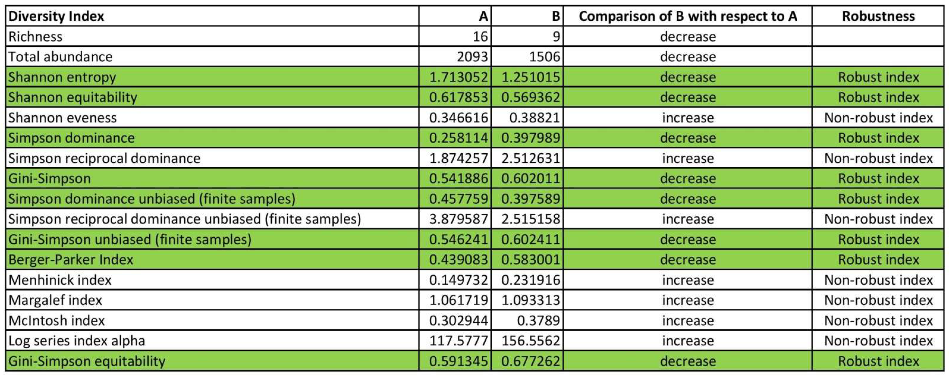
The assessment criterion for each diversity index was its robustness, i.e., whether its conclusion regarding the biodiversity pairwise comparison (increase, decrease, or no change) was consistent with the conclusion of both of the two main diversity components (richness and abundance).

The pairs of values refer to the values of diameters, heights, or volumes of the trees of two different forests, measured at the same time, or to the values of the same variables in the same trees of the same forest at two different times. So, the pairwise comparison is the comparison of two different regions at the same time, or the comparison of two different times for the same region, regarding the trees’ diameter, height, or volume.

The method by which we examined the indices’ robustness, i.e., their consistency in indicating an increase or decrease in biodiversity over pairwise comparisons, was the bootstrap method [28]. The bootstrap method is a resampling approach used to estimate statistics on a population by sampling a dataset with replacement. To guarantee that useful statistics, such as the mean, standard deviation, and standard error, can be derived from the sample, the number of repetitions must be sufficient in size. In an ideal scenario, the repetitionswould be as high as is practically achievable given the available time and resources, with hundreds or thousands of iterations. Nonetheless, it is crucial to remember that the number of repetitions required for precise estimations can vary based on the time and resources available as well as the complexity of the dataset; it is a waste of resources to conduct a thorough analysis of a homogeneous data set [29,30].

According to [31], the number of iterations that are suggested for common use is 599. This number serves as a rule of thumb. In this study, 100,000 samples of data relevant to forests (trees’ diameters, heights, and volumes) were analyzed.

To perform the bootstrap method, we used the bootstrap resampling technique available in NumPy [32] and scikit-learn [33] Python libraries.

3. Results

After conducting a bootstrap analysis on 100,000 samples of data related to forests (tree diameters, heights, and volumes), it was determined that eight diversity indices described in Table 1 yield robust results, meaning that they consistently showed an increase or decrease in biodiversity over pairwise comparisons, i.e., when comparing the same region at two different times or two different regions at the same time, in terms of biodiversity. These indices are (as numbered in Table 1) as follows:

3	Shannon entropy;
4	Shannon equitability;
6	Simpson dominance;
8	Gini–Simpson;
9	Simpson dominance unbiased (finite samples);
11	Gini–Simpson unbiased (finite samples);
12	Berger–Parker Index;
17	Gini–Simpson equitability.

Figure 1 depicts a snapshot of these 100,000 samples (one random run out of the 100,000). Ref. [34] used these eight indices, which showed to be robust in terms of forest data. The columns labeled “A” and “B” denote either the diversity indices derived from data collected at the same forest, at times A and B, respectively, or the diversity indices derived from data collected at the same time, at forests A and B, respectively. Hence, for instance, the message “decrease” in the column titled “Comparison of B with respect to A” indicates that the corresponding diversity index of a forest decreases in time B relative to the diversity index in preceding time A or that, at a given time, the corresponding diversity index of forest B is less than that of forest A.

These indices were shown to be robust; that is, their results for comparing biodiversity pairs (increase, decrease, or no change) matched both of the two main diversity components (richness and abundance) across the whole set of 100,000 samples of tree diameter, height, and volume.

4. Discussion

In this review article, 17 of the most popular indices are presented, allowing the reader to choose which ones are most applicable to their particular set of data (genetic, econometric, sociometric, etc.). For these indices, we note which proved robust and which did not when applied to forest data. Readers may find the following table and the supplementary BiodiversityIndicesCalcExample.xlsx template helpful in the selection, application, and interpretation of diversity indices and useful in choosing the robust indices for their particular set of data (genetic, econometric, sociometric, etc.). In this template, readers can type their own data in columns A and C (highlighted in green) of spreadsheets “A” and “B” and see if the indices are robust, looking at the spreadsheet “comparison”. For demonstration purposes, values in the C column of spreadsheets “A” and “B” of the BiodiversityIndicesCalcExample.xlsx template are generated with a random number generator (“randbetween” formula). The reader can see how the “comparison“ spreadsheet changes when refreshing the “randbetween” formulas by pressing the F9 key.

Spreadsheets A and B correspond either to samples of two different populations (A and B) or to the same population from which we took samples at times A and B. The purpose of using a random number generator is to simulate the variability that can occur in real-world data. We can see how different random values in spreadsheets A and B affect the biodiversity indices in the “comparison” spreadsheet by refreshing the formulas. This allows us to analyze and compare the biodiversity of the two populations or the changes in biodiversity over time within a single population.

It should be noted that a diversity index is characterized as “robust” when it gives the same result (increase, decrease, or no change in biodiversity when comparing A and B) as the richness and abundance, which are the two components of biodiversity. This implies that if the diversity index of spreadsheets A and B aligns with the changes in richness and abundance then it can be considered a robust measure of biodiversity. Regardless of the specific index employed, this robustness guarantees that the diversity index appropriately captures changes in biodiversity. This is important because different measures of biodiversity may focus on different aspects, such as species composition or genetic diversity. By aligning with changes in richness and abundance, the diversity index captures the overall changes in biodiversity across these different aspects. Therefore, researchers can confidently use the diversity index as a reliable indicator of biodiversity changes in their studies.

In the specific context of calculating biodiversity using proxies or surrogates for biodiversity assessment in forest areas, we could not identify comparable studies that directly align with our research focus. It appears that limited research has specifically examined the use of diversity indices as proxies for biodiversity assessment in the context of forest management. We believe that our findings contribute to filling this research gap by specifically assessing the feasibility and applicability of diversity indices as proxies for biodiversity in forest management. Although it is challenging to make direct comparisons with other studies due to the unique focus of our research, our findings provide insights into the effectiveness of these indices in capturing biodiversity patterns within forested areas.

5. Conclusions

This work summarizes 17 diversity indices and discusses the results of a bootstrap analysis conducted on 100,000 samples of forest data. Eight indices were found to yield robust results. These indices include Shannon entropy, Shannon equitability, Simpson dominance, Gini–Simpson, Simpson dominance unbiased (finite samples), Gini–Simpson unbiased (finite samples), Berger–Parker Index, and Gini–Simpson equitability. Based on this, we can safely conclude that these eight indices will show an increase, decrease, or no change in biodiversity when the biodiversity component is trees’ DBH, height, or volume, and when comparing the biodiversity values of two different forests measured at the same time or two consecutive biodiversity values referring to the same forest. It is important to select robust diversity indices for different types of data that align with changes in richness and abundance, which are the two main components of biodiversity. Robust diversity indices that give the same result as richness and abundance ensure that they accurately capture changes in biodiversity across different aspects so researchers can confidently use them as reliable indicators of biodiversity changes in their studies.