Data Structures and Algorithms for k-th Nearest Neighbours Conformational Entropy Estimation

Abstract

Entropy of multivariate distributions may be estimated based on the distances of nearest neighbours from each sample from a statistical ensemble. This technique has been applied on biomolecular systems for estimating both conformational and translational/rotational entropy. The degrees of freedom which mostly define conformational entropy are torsion angles with their periodicity. In this work, tree structures and algorithms to quickly generate lists of nearest neighbours for periodic and non-periodic data are reviewed and applied to biomolecular conformations as described by torsion angles. The effect of dimensionality, number of samples, and number of neighbours on the computational time is assessed. The main conclusion is that using proper data structures and algorithms can greatly reduce the complexity of nearest neighbours lists generation, which is the bottleneck step in nearest neighbours entropy estimation.

1. Introduction

Entropy is a key quantity for statistics, physics, chemistry, and computer science. Its meaning has been given in different contexts, but it can be basically traced to its probabilistic definition as described hereafter.

For a large number of biophysical processes, including solvation, association, and conformational transitions, it is very difficult to provide a theoretical estimation of the change of entropy.

Molecular dynamics simulations can, in optimal situations, sample thermodynamic ensembles of configurations and, in this context, estimation of entropy changes leads to an immediate estimation of free energy changes because enthalpy is directly estimated in simulations by the molecular mechanics energy, available through the force field.

Free energy is typically obtained by defining a path or a collective variable which can vary continuously between the initial and the final states [1,2,3,4]. Such pathway methods have some limitations because thermodynamic ensembles should be obtained at each discretized point along the path, which requires long simulations, and moreover the obtained entropy cannot be related to single or groups of degrees of freedom.

For this reason, entropy estimation from end-point simulations [1,5] has attracted interest.

The main difficulty in entropy estimation is related to the treatment of a large number of non-independent variables, which require appropriate approximations. A great reduction in complexity is achieved by treating solvation implicitly through continuum methods which provide, through the temperature dependence of the potential of mean force, solvation entropy estimation [5,6,7]. The entropy of the solute is then approximated by the entropy of the multivariate torsional angles distribution [8]. It is estimated that the changes in the entropy associated with bonds and angles is about one order of magnitude smaller than that associated with torsion angles [9,10].

Being left with only torsional angles as conformational variables, a straightforward approach is to discretize the probability density functions (pdf) in histograms and to compute the entropy for the discrete distribution. The approach is, however, prohibitive with the increasing number of torsion angles considered, because either most multidimensional bins will contain 0 or few samples, or they will be so large that resolution will be reduced with consequent overestimation of entropy.

A way to circumvent this problem is to consider only pairs of torsion angles and estimating the total entropy using either the mutual information expansion (MIE) method as proposed by Gilson and coworkers [11] or approximating it using an upper bound as provided by the mutual information spanning tree (MIST) method, as proposed by Tidor and coworkers [12,13].

If the mutual information of more than two variables is non-negligible, the above approach will not provide a tight bound to entropy and, therefore, groups of variables of higher dimensions must be taken into account.

Methods for non-parametric density and entropy estimation have been reviewed before [14,15,16,17], and the reader is referred to these comprehensive reviews. Histogramming the variables’ space and assuming a constant density inside each bin may be considered as a simple way to estimate the density function. A flexible extension of this idea is provided by kernel density estimators (kde). Constant, Gaussian, and other kernels are currently used in many fields, notably machine learning [17]. For entropy estimation, any bias introduced at the density estimation step is typically corrected afterwards. The approach leads, however, to difficulties when the dimensionality of the problem increases, because multidimensional integration of the density function must be performed. For this reason re-substitution methods, which replace the integral by a sum over the available samples, for an unbiased sampling, are useful [14].

The k-th nearest neighbours (briefly referred as: kNN) method [18,19], which generalizes, in a rigorous way, the idea of estimating the multivariate probability density at each sample by counting how many other samples are found within a given volume around that sample and finally averaging over the samples, shares ideas with the histogram density estimation, the kernel density estimator and re-substitution methods, previously proposed.

In the kNN method, however, the density is estimated only at the available samples, and instead of fixing the volume within which neighbours are counted, the number of neighbours is fixed and the minimum volume enclosing exactly that number of neighbours is evaluated. The entropy is then evaluated using the distance to the k-th neighbour, which overcomes the need of using a kde, simplifying calculations. In such a way, the density at each sample is estimated in a simple way using the same number of samples and the volume is flexibly adapted to the density of points, i.e., it will be small where samples are dense and large where there are few samples. This procedure ensures that the resolution of the distribution is matching as far as possible the number of samples available.

This adaptive feature appears particularly interesting when dealing with large multidimensional spaces, such as the ones describing macromolecular conformation and solvent configurations.

The method has been used by us and others before for estimating conformational [8,9,20,21,22], translational/rotational [9,23,24,25], and solvation [23,26,27,28] entropy.

There are at least a couple of bottlenecks in this approach: the first is that a large number of independent samples must be acquired, which means long simulation; the second, and most important, is that a naive implementation would require the computation of a number of distances quadratic in the number of samples.

In this article, we address the data structures and algorithms for nearest neighbours generation which allow a substantial reduction in computational time and, in particular, for periodic variables, such as torsion angles.

Compared to the literature existing on this subject (see, e.g., the review by Brown et al. [29]) here we address the implementation and application of the methods to the typical dimensionality and number of samples found in the estimation of entropy from snapshots extracted from biomolecular dynamics simulation trajectories, showing advantages and limitations of kNN entropy estimation for typical biophysical systems.

2. Materials and Methods

2.1. Entropy

Given a tuple $\overrightarrow{x}=(x_1,x_2,\cdots ,x_d)$ of d variables, the entropy of a multivariate probability density function $p\left(\overrightarrow{x}\right)$ is defined by:

$$S=-{\int }_{V_d}p\left(\overrightarrow{x}\right)log\left(p\left(\overrightarrow{x}\right)\right)d\overrightarrow{x}$$

(1)

where $V_d$ is the multidimensional volume of the set of tuples of points admissible for the d variables. The logarithm is taken for convenience here as the natural logarithm function.

Based on the above formula the entropy may be also defined as the expectation value of $-log\left(p\left(\overrightarrow{x}\right)\right)$, i.e.,

$$S=-\langle log\left(p\left(\overrightarrow{x}\right)\right)\rangle$$

(2)

2.2. Entropy Estimation Using the kNN Method

Let us assume to have a set of n points in d-dimensions $V=\{{\overrightarrow{x}}_1,{\overrightarrow{x}}_2,\cdots ,{\overrightarrow{x}}_n\}$. Let us focus on one of them, say ${\overrightarrow{x}}_i$. The k-th nearest neighbours (kNN) method estimates the probability density $\widehat{p}$ at each sample i by considering the minimal volume of a d-dimensional ball enclosing its k nearest neighbour samples. If such volume is $V_{i,k}$, then the density at sample i, under the assumption that it is approximately uniform in the neighbourhood of the sample, is estimated, in a naive way, by:

$$\widehat{p}\left({\overrightarrow{x}}_i\right)\approx \frac{k}{n{V}_{i,k}}$$

(3)

and, again in a naive way, if samples are taken with probability $p\left(\overrightarrow{x}\right)$, the entropy may be estimated as

$$\widehat{S}=-\langle log\left(p\left(\overrightarrow{x}\right)\right)\rangle \approx -\frac{{\sum }_{i}log\widehat{p}\left({\overrightarrow{x}}_i\right)}{n}=-log\left(k\right)+log\left(n\right)+\frac{{\sum }_{i}log\left(V_{ik}\right)}{n}$$

(4)

The naive approach may be rigorously treated [18,19] and leads to the correct form of the Equation (4) which is:

$$\widehat{S}=-L_{k-1}+\gamma +log\left(n\right)+\frac{{\sum }_{i}log\left(V_{ik}\right)}{n}$$

(5)

where $L_k$ is defined by $L_0=0$ and $L_i=L_{i-1}+1/i$ and $\gamma$ is the Euler–Mascheroni constant (0.5772…). Note that $L_{k-1}-\gamma$ replaces $log\left(k\right)$ of the naive Equation (4).

Equation (5) provides an unbiased estimation of the entropy of the probability density function $p\left(\overrightarrow{x}\right)$ based on the kNN method.

It is important to note that in non-Euclidean spaces, such as those of single and pairs of translation/rotations, the computation of both the distances and the corresponding volumes of the balls with those distances as radii might be non-obvious.

The other space relevant for conformational entropy is the space of torsional angles for which we must take only into account the periodicity in the definition of the distance.

2.3. Data Structures and Algorithms for k-th Nearest Neighbours Computation

Given a set V of n points in a d dimensional space, a semimetric is a function $f:V\times V\to \mathcal{R}$ such as that for all points $\overrightarrow{x},\overrightarrow{y}\in V$:

• $f(\overrightarrow{x},\overrightarrow{x})=0$;
• $\overrightarrow{x}\ne \overrightarrow{y}\Rightarrow f(\overrightarrow{x},\overrightarrow{y})>0$;
• $f(\overrightarrow{x},\overrightarrow{y})=f(\overrightarrow{y},\overrightarrow{x})$.

Given $\overrightarrow{x},\overrightarrow{y},\overrightarrow{z}\in V$ we say that $\overrightarrow{y}$ is nearer to $\overrightarrow{x}$ than $\overrightarrow{z}$ if $f(\overrightarrow{x},\overrightarrow{y})<f(\overrightarrow{x},\overrightarrow{z})$.

In this work, we will consider both Euclidean spaces, where f is the Euclidean distance, and non-Euclidean spaces, where f is a generic distance function.

Given a semi-metric and the set of points V, the all-k-nearest-neighbours problem (all-k-nn in short) is the problem of finding the k nearest neighbours of each point $\overrightarrow{x}\in V$.

In this section, we briefly review the main approaches to solve this problem; in particular, after describing a straightforward implementation we show how to exploit two popular data structures for this kind of problems.

Before continuing, let us recall two basic results. If we can do comparison operations on two numbers in constant time, the following statements hold:

• Given a list of n numbers, the sorting problem can be optimally solved in $\mathsf{\Theta }(nlog(n\left)\right)$ time.
• Given a list of n numbers and an index i, the selection problem (i.e., the problem of finding the i-th smallest number) can be solved in $O\left(n\right)$ time (for example, using the Medians-of-medians algorithm [30]). It follows that the median of a list can also be calculated in linear time.

Considering the problem in one dimension, it is well known [31] that there is a $\mathsf{\Omega }(nlog(n\left)\right)$ lower bound in the algebraic decision tree model of computation. This is an important result that we can use to judge the goodness of each algorithm we are going to discuss.

2.3.1. Naive Algorithms

We can distinguish cases with $d=1$ and $d>1$ to provide two different naive implementations with different run-time complexities.

One-Dimensional Approach

If all the points are in one dimension, a straightforward implementation is the following:

• Perform an ordering in $\mathsf{\Theta }(nlog(n\left)\right)$ time.
• For each point select the k-th neighbours in $\mathsf{\Theta }\left(k\right)$ time.

The overall complexity is then $\mathsf{\Theta }(nlog(n)+kn)$ which is optimal considering the lower bound discussed above. Note that once the points are ordered, considering a point p in position i, the nearest neighbour of p is either in position $i+1$ or in position $i-1$.

Multidimensional Approach

If the points are in d dimensions, with $d>1$, the previous approach stops working. A straightforward implementation, in this case, is the following.

For each point p:

• Calculate all the distances between p and all the other points in $\mathsf{\Theta }\left(nd\right)$ time.
• Find $p_k$, a point that has the k-th smallest distance from p using a linear time selection algorithm.
• Select all the j points whose distance from p is strictly less than $d(p,p_k)$ and then arbitrary select $k-j$ points whose distance is exactly equal to $d(p,p_k)$, if there are more than one such points.

The overall complexity is then $\mathsf{\Theta }\left(n\right)(\mathsf{\Theta }\left(nd\right)+O\left(n\right)+O\left(n\right))=\mathsf{\Theta }\left(d{n}^2\right)$ which is much worse than the single dimension approach and it is not even near to the lower bound discussed.

2.3.2. Space Partitioning Algorithms

The use of tree data structures can be exploited to avoid the explicit computation of $\mathsf{\Theta }\left(n^2\right)$ distances. As reported in Algorithm 1, first the tree is built and then for each point p it is traversed looking for its neighbourhood. In the next sections, we describe K-D Trees and vantage point (VP) Trees which are balanced binary trees that work with multidimensional points. In these trees, the root node represents the entire set V and each internal and leaf node represents a subset of V. Each point is memorized in a single leaf node and each leaf node may contain at maximum b points where $b>1$.

In Algorithm 2, we give a general recursive function to build such a tree starting from a set of points. In each call, we construct a node u and we recursively build $u.\mathtt{left}$ and $u.\mathtt{right}$ by splitting the input point set into two new sets according to the properties of the tree structure. When the cardinality of the input set is less or equal than b, a leaf node (which will store all the remaining points) is created. If, at each call, we spend $\mathsf{\Theta }\left(nd\right)$ time for the splitting process, then the equation of run-time complexity of Algorithm 2 is the following:

$$\begin{array}{c}T\left(n\right)=\left\{\begin{array}{cc}\mathsf{\Theta }\left(1\right)\hfill & \mathrm{if}n\le b\hfill \\ T\left(\alpha n\right)+T\left(\beta n\right)+\mathsf{\Theta }\left(nd\right)\hfill & \mathrm{else}\hfill \end{array}\right.\hfill \end{array}$$

(6)

where n is the number of input points and $\alpha$ and $\beta$ are the fractions of points that will be stored, respectively, in the left and right sons.

We can now define the run-time complexity of Algorithm 1 as:

$$A(n,k,d)=T\left(n\right)+nS(n,k,d)$$

(7)

where $T\left(n\right)$ is the time taken by the tree construction algorithm (as seen in Equation (6)) and $S(n,k,d)$ is the time taken by a single execution of the query algorithm (which we will describe for both K-D Trees and VP Trees).

Algorithm 1 General all-k-nn algorithm using a tree structure

functionALL-KNN($points,n,k,d$)     $T\leftarrow$BUILD-TREE($points$)                     ▹ Tree building     $sol\leftarrow$NEW-ARRAY(n)                 ▹ Space allocation for solution      for each $p\in points$  do             $so{l}_p\leftarrow$QUERY($p,T.\mathtt{root},k$)                 ▹ Tree traversal      end for      return $sol$ end function

Algorithm 2 General tree construction

functionBUILD-TREE($points$)      if $\left|points\right|\le b$  then          return MAKE-LEAF($points$)      end if     $u\leftarrow$ MAKE-INTERNAL-NODE     $point{s}_{\mathtt{left}}\leftarrow \left\{q\in points|q\mathrm{must}\mathrm{be}\mathrm{memorized}\mathrm{in}\mathrm{the}\mathrm{left}\mathrm{son}\right\}$     $point{s}_{\mathtt{right}}\leftarrow \left\{q\in points|q\mathrm{must}\mathrm{be}\mathrm{memorized}\mathrm{in}\mathrm{the}\mathrm{right}\mathrm{son}\right\}$     $u.\mathtt{left}\leftarrow$BUILD-TREE$\left(point{s}_{\mathtt{left}}\right)$     $u.\mathtt{right}\leftarrow$BUILD-TREE$\left(point{s}_{\mathtt{right}}\right)$      return u end function

2.3.3. K-D Tree

The Data Structure

Considering Euclidean spaces, the best-known structure to solve the all-k-nearest-neighbours problem uses the so-called K-D Tree. The K-D Tree was initially developed by Bentley [32] and later on it was proposed in an optimized version by Bentley, Friedman, and Finkel with the specific purpose of efficiently solving the kNN problem [33]. Each internal node is endowed with two additional fields: the discriminator which is an integer in the interval $[1,d]$, and the partitionValue which is a real number. The semantics is the following: for each node u let $j=u.\mathtt{discriminator}$, for each point $p=(p_1,\cdots ,p_d)$ stored in the subtree rooted in $u.\mathtt{left}$ it must hold $p_j<u.\mathtt{partitionValue}$. Similarly, if p is contained in the subtree rooted in $u.\mathtt{right}$ it must hold $p_j\ge u.\mathtt{partitionValue}$. To build a balanced tree, at each recursive call in Algorithm 2, first we calculate the projection of all the input points onto the coordinate indicated by the discriminator and then the partitionValue is chosen to be the median of those values so that the input points are split into two balanced sets. To maximize the information contained in each node splitting, the discriminator is chosen to be the coordinate with maximum spread. Substituting $\alpha =\beta =\frac{n}{2}$ in Equation (6), we can see that we can build a balanced K-D Tree in $\mathsf{\Theta }(dnlog\left(\frac{n}{b}\right))$ time. Note that at each internal node, the $\mathtt{partitionValue}$ defines lower and upper bounds on the value of the $\mathtt{discriminator}$ coordinate for each point contained in the two sons. We say that each node is associated to a domain and the domain of the root is $(-\infty ,+\infty )$ for each coordinate.

The Search Algorithm

We now describe the query algorithm, as proposed in [33]. The query algorithm is recursive and takes as input a point $p=(p_1,\cdots ,p_d)$, a node u and the value of k.

During the search, we have the need to compute many times the best k-th nearest neighbours so far encountered. To satisfy the requirement we use a data structure called max-priority queue.

In this case, we can use a max-priority queue of length k and we will use an efficient implementation called max-heap. With this setup, we are able to retrieve the k-th nearest neighbour yet found in constant time, and we can perform insertion and deletion operations in $O(log(k\left)\right)$ time.

At each recursive call, we visit the node u. If u is a leaf, all the points stored are examined and the queue may be updated with nearer neighbours for p.

If u is an internal node, if $p_{u.\mathtt{discriminator}}\ge u.\mathtt{partitionValue}$ we first recursively visit $u.\mathtt{right}$, otherwise, we first visit $u.\mathtt{left}$. When the control returns from the recursive call we have to decide if a call on the opposite son is necessary.

We consider the hyper-sphere centred in p with radius the k-th nearest distance from p found in the priority queue. If the hyper-sphere intersects the domain of the node not already visited, then the second recursive call must be performed.

After visiting node u we check if it is necessary to continue the search. If the hyper-sphere previously described is completely contained in the domain of u, then the priority queue contains the real k neighbours for p and the algorithm will terminate.

Analysis

In [33] it is shown that during a search, the average number of points examined R is bounded by $R\le {(k^{\frac{1}{d}}+b^{\frac{1}{d}})}^d$. Note that R is independent of n, so, given values k and d, the time taken by the query algorithm is proportional to the height of the tree, and since the tree built is balanced, its height is proportional to $log\left(n\right)$. We can conclude that the expected time to solve the all-k-nn problem is $O(dnlog(n\left)\right)$, however, this is true just for small values of d and k. The real worst case of the implementation is $O(d{n}^{2}log\left(k\right))$. The intuitive meaning is that for some values of d and k, the query algorithm must perform 2 recursive calls for each node, so all the $\mathsf{\Theta }\left(n\right)$ nodes of the tree are visited.

2.3.4. VP Tree

The Data Structure

The good behaviour of the K-D Tree approach might sensibly degrade outside Euclidean spaces (e.g., spaces with periodic boundary conditions [29]). VP Trees were proposed by Yianilos [34] for dealing with generic metric spaces.

Instead of the discriminator and the partitionValue of K-D Trees, each node of a VP tree has the following two additional attributes: the vantagePoint which is a point and the radius which is a real value.

The semantics is the following: for each node u let $vp=u.\mathtt{vantagePoint}$, for each point $p=(p_1,\cdots ,p_d)$ stored in the subtree rooted in $u.\mathtt{left}$ it must hold $d(p,vp)<u.\mathtt{radius}$. Similarly, if p is contained in the subtree rooted in $u.\mathtt{right}$ it must hold $d(p,vp)\ge u.\mathtt{radius}$. In each call of the tree construction algorithm, the radius is chosen to be the median value of the list obtained considering the distances between the vantagePoint and all the input points. The vantagePoint can be chosen in various ways but the simplest method is to choose a random point from the input point set. As the K-D Tree, the VP Tree can be built in $\mathsf{\Theta }(dnlog\left(\frac{n}{b}\right))$ time.

The Search Algorithm

We now describe the query algorithm for the VP Tree as proposed in [34]:

• The input is the same as for K-D Tree.
• We maintain a max-priority queue of length k with the same meaning as for K-D Tree.
• In each call, we visit the node u, and if u is a leaf node the steps performed are the same as for K-D Trees.

We maintain a global variable $\tau$ which bounds the maximum distance from the query point p and its k-th nearest neighbour. $\tau$ is used to decide where to search and its initial value is $+\infty$, indicating that the neighbours of p could be everywhere in the space.

During the visit of u, we calculate $f=d(p,u.\mathtt{vantagePoint})$, the distance from p and $u.\mathtt{vantagePoint}$. The first son visited is the one concordant to the search of p in the tree, in particular, if f is less than $u.\mathtt{radius}$, the first son visited is $u.\mathtt{left}$, otherwise, it is $u.\mathtt{right}$.

After the control returns from the first recursive call, we have to decide if we have to visit the second son. We consider the space between the hyper-sphere centred in $u.\mathtt{vantagePoint}$ with radius $u.\mathtt{radius}+\tau$ and the hyper-sphere with the same centre and radius $u.\mathtt{radius}-\tau$.

If, after the traversal of the tree rooted in the first son, p is contained in the described space, then we must visit the other son. Intuitively, if p is distant from $u.\mathtt{vantagePoint}$ exactly $u.\mathtt{radius}$, we trivially have to visit both sons, in fact, the hyper-sphere centred in p with radius $\tau$ will always intersect both sons’ subspaces. If the distance of p and $u.\mathtt{vantagePoint}$ is near to $u.\mathtt{radius}$ we visit the second son just in case the hyper-sphere centred in p with radius $\tau$ intersects its associated subspace.

Note that when the control returns from the first visited son, the value of $\tau$ might have decreased. Once the algorithm has terminated, the max-priority queue contains the neighbours for p.

Analysis

The run-time complexity of the all-k-nn algorithm which uses the VP Tree is the same as the one discussed for the K-D Tree, as can be shown using similar arguments [34]. So we still obtain $O(dnlog(n\left)\right)$ expected time and $O(d{n}^{2}log\left(k\right))$ worst case. Experimental results show that the KD Tree performs slightly better in Euclidean spaces, but the VP Tree algorithm can be used in any metric space and we can still solve the neighbourhood problem with the same complexity.

2.4. Software Availability

The software used for this article has been entirely written in C. It is available on the GitHub repository (https://github.com/robyBorelli/nearest-neighbours-package, accessed on 12 October 2022) and distributed under the license GNU GPL v3. Instructions on compilation and usage are deposited on the GitHub repository together with example files.

3. Results

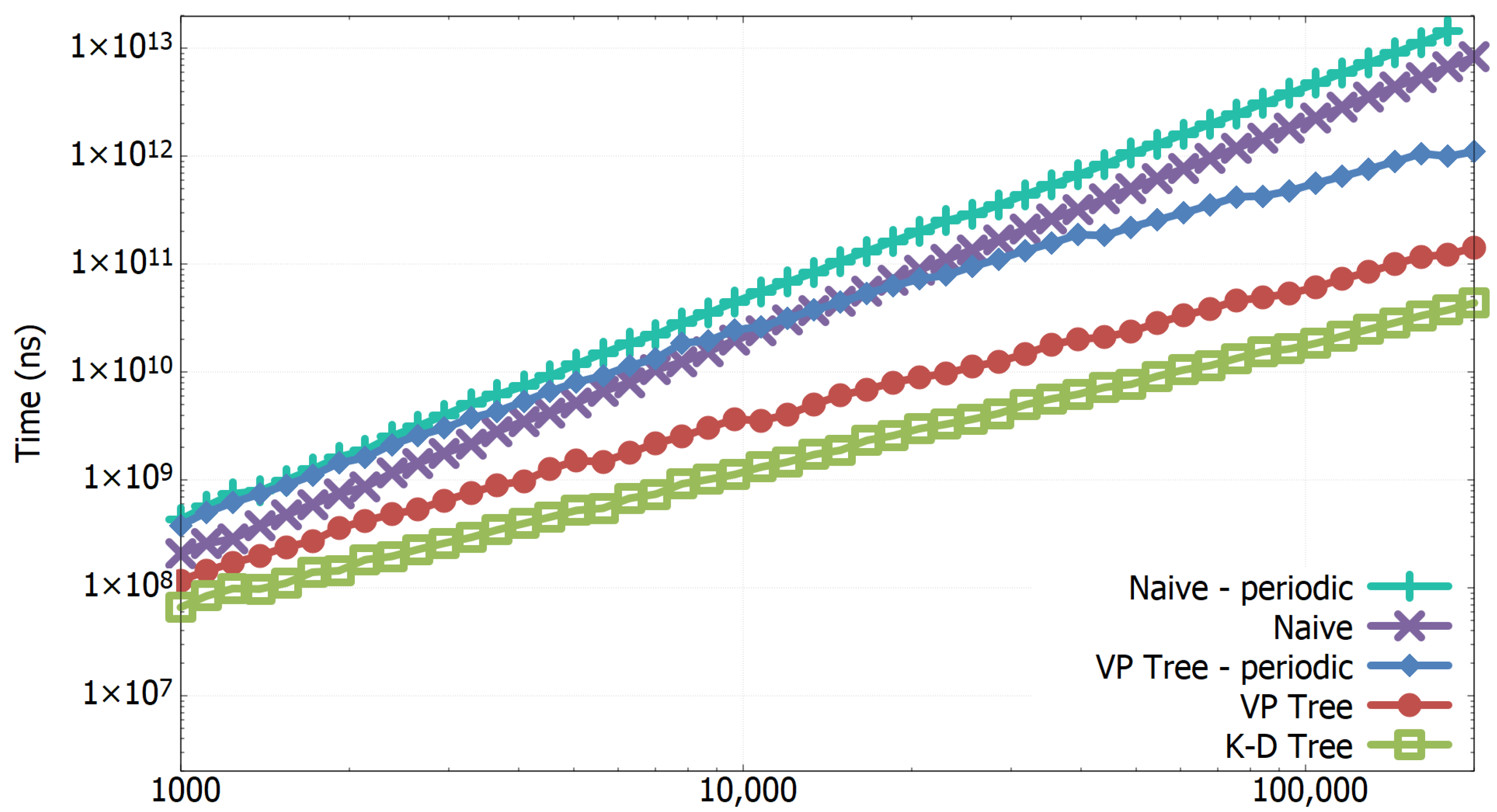
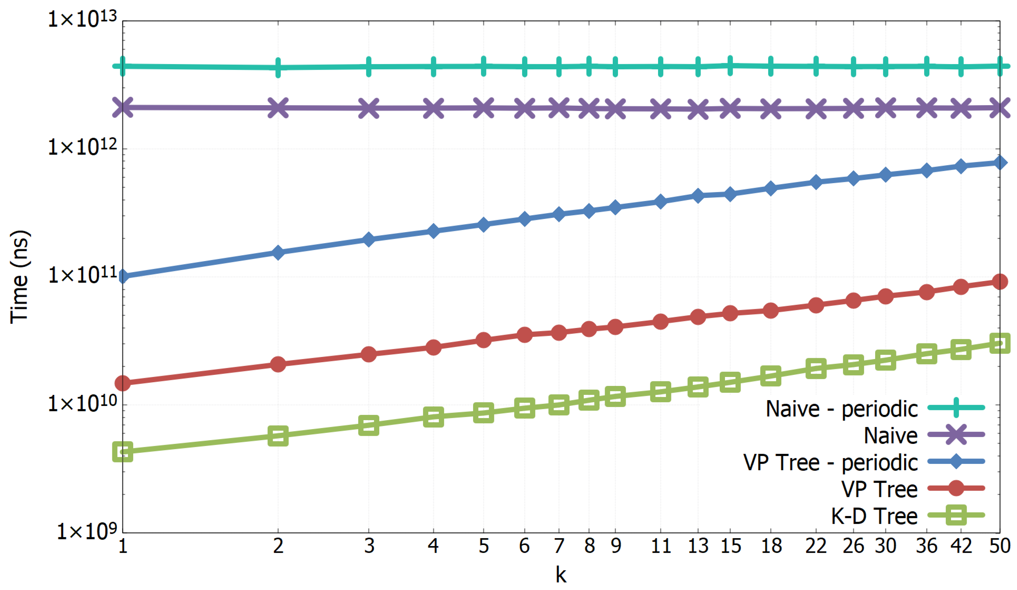
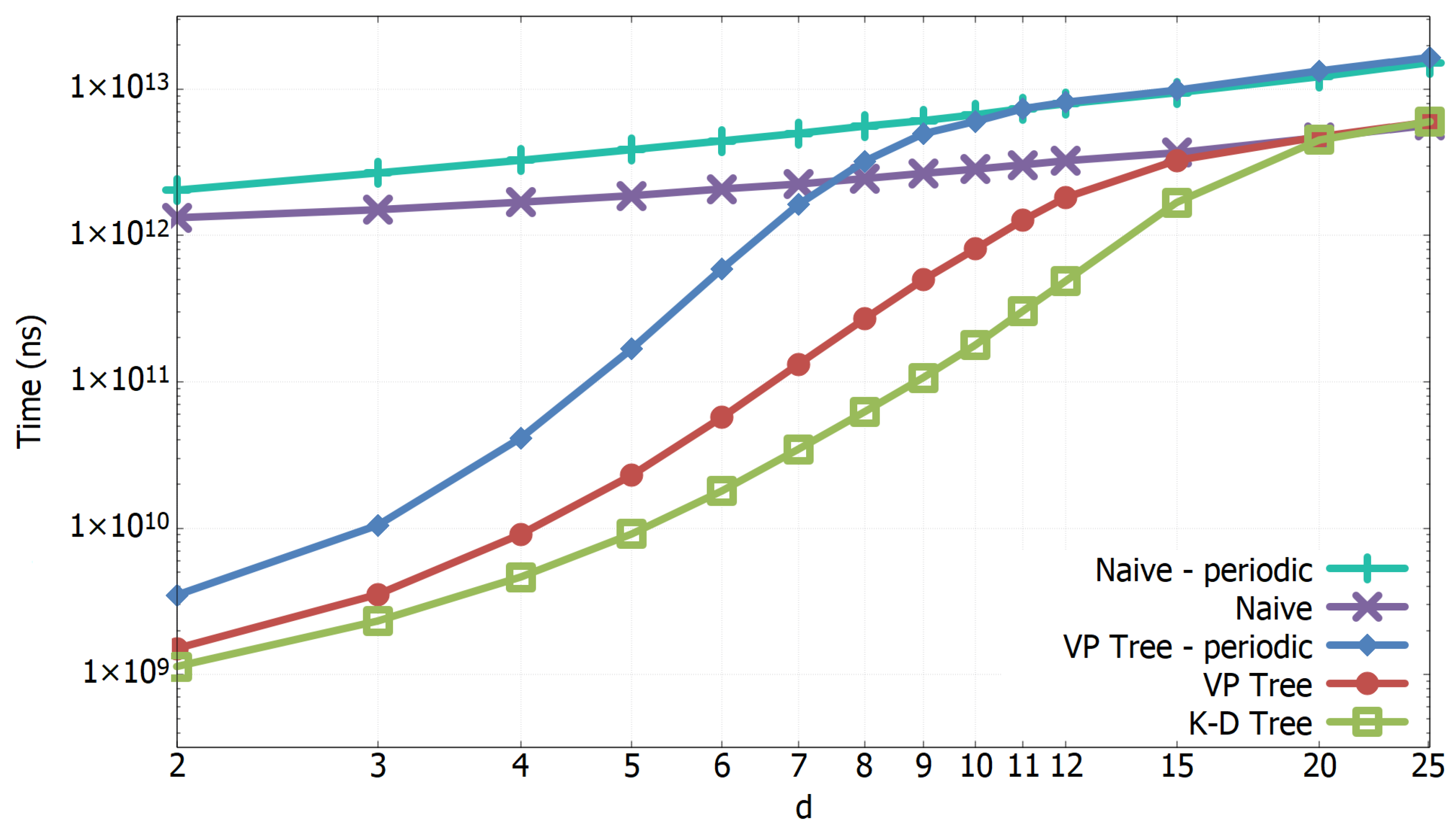
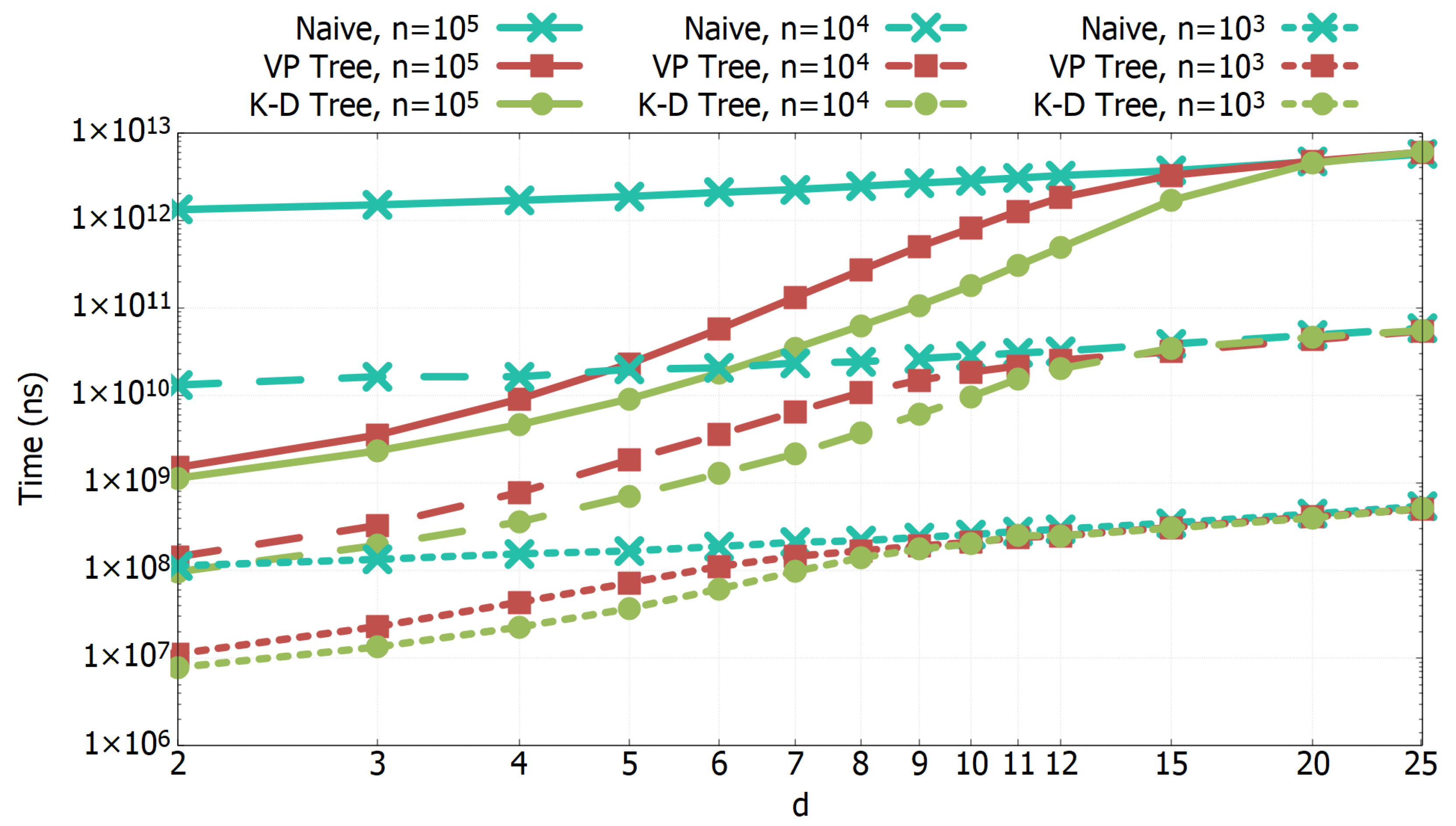
3.1. Experimental Results of All-k-nn Algorithms

To experimentally verify the promising theoretical results of the all-k-nn algorithms of the previous sections, we wrote a C implementation and then run three comparison tests which are representative of common cases in molecular dynamics and databases’ analysis.

We implemented the following algorithms: Naive, K-D Tree, and VP Tree. We call Naive the all-k-nn algorithm which computes all the $\mathsf{\Theta }\left(n^2\right)$ distances between points. The Naive and VP Tree algorithms have also been implemented in the variant that works in spaces with periodic boundary conditions. Referencing to the Naive algorithm may be questionable because neighbour lists are computed, e.g., in MD simulation, by more efficient algorithms (e.g., cell lists [35]) than the naive one, but such algorithms are not applied to higher dimensions with the same efficiency, because the number of cells needed grows exponentially with d. For this reason, tree structures have been widely used for higher dimensions [29]. Therefore, we kept as a reference the Naive algorithm which is straightforward to apply in all dimensions.

For each test, we present a double logarithmic scale plot which shows the dependency of the execution-time with respect to parameters n, k, and d. We recall that in a double logarithmic scale, polynomial functions are displayed as straight lines and straight lines with the same inclinations are polynomials with the same degree.

In order to test the algorithms in a realistic scenario for estimating conformational and configurational entropy from molecular dynamics simulation trajectories, we consider that a typical sample may entail $n=$ 10,000 to 100,000 samples, the dimension d of grouped variables may be typically in the range 4 (the typical amino acid torsional angles) to 12 (12 variables are needed to describe pairs of rigid water molecules) and k may be in the range of 10 to 20 depending on the resolution. All tests reported hereafter take these numbers in consideration as references.

In Figure 1, we compare the algorithms as the number of points grows. We have taken the time of 50 executions from $n=$ 1000 to $n=$ 200,000 with $k=20$ and $d=6$. We observe that Naive algorithms show quadratic performances, as expected, and that the tree-based algorithms lines’ have the same inclination indicating a linearithmic growth; the K-D Tree algorithm has a lower multiplicative constant and so it performs best. In Figure 2, we show the algorithms’ comparison as the size of the neighbourhood is increased, in particular, we use values of k from $k=1$ to $k=50$. The asymptotic time of Naive algorithms is independent of k and so we see no aggravation of efficiency as k becomes larger. The tree-based algorithms have a slight decrease in performance but this is marginal considering $k<<n$. We must notice that choosing sufficiently large values of k will eventually lead tree-based algorithms to quadratic performances. Intuitively, the greater the k, the more nodes of the tree will be visited, in particular, with large-enough values of k, for each point p, the tree traversal will pass through $\mathsf{\Theta }\left(n\right)$ nodes and so the algorithm will degenerate to an exhaustive search with quadratic complexity.

In Figure 3, the limitation of tree-based algorithms with increasing dimensionality is illustrated. The naive algorithms’ performances grow linearly with the number of dimensions d. We observe that starting from $d=1$, the time of tree-based algorithms exponentially becomes bigger so the addition of 1 dimension will cause at least a doubling in time. This behavior continues until the same performance of Naive algorithms is reached and from that point on the growth is linear with d. This phenomenon is called curse-of-dimensionality: each algorithm that solves the all-k-nn problem will degenerate in at least a quadratic search starting from certain values of d. This problem affects all the algorithms yet discovered. Based on combinatorial arguments, when we consider uniformly distributed samples, we may expect the algorithm efficiency to be lost when $d\in \mathsf{\Theta }\left({log}_2\left(n\right)\right)$. For $n=$ 100,000 this amounts to $d=17$, which is in the range where K-D Tree and VP Tree algorithms’ curves merge with the Naive algorithm one in Figure 3. This limitation was further confirmed for other values of n and d, as shown in Figure 4. With $n=$ 100,000 and $k=20$, the VP Tree (periodic) is still convenient for $d=10$ and it reaches the quadratic search with $d=11$. The VP Tree (non-periodic) and the K-D Tree are convenient even for $d=12$, with the same values of n and k. Even if asymptotic times are the same for the K-D Tree and the VP Tree, we notice that the curse-of-dimensionality is a little bit more accentuated with the VP Tree structure: with $d=12$, $n=$ 100,000, and $k=20$ we observe that the VP Tree search is more than 3 times slower than the K-D Tree one.

In all three tests, we can notice the advantage provided by the VP Tree structure: it asymptotically performs the same with Euclidean and non-Euclidean spaces although the multiplicative constant is lower for the Euclidean case.

3.2. Entropy of Amino Acids in Random Conformations

In our previous report [22], we studied the entropy of all amino acids in coil conformation (i.e., not in $\alpha$-helix or $\beta$-strand conformation, as obtained by DSSP analysis [36], in the implementation given by Vriend and coworkers [37]). The dataset of structures used in this work was obtained in a previous work (Mahmood et al., submitted) by downloading non-redundant sequences (at less than 40% identity) from the culling server Pisces [38] with resolution of $<4.0$ Å and R-factor $<1.0$. The set entails 27,316 sequences. Only amino acids for which all torsion angles could be computed were considered.

For each amino acid the ensemble of all conformations available in the dataset was built and the entropy was computed, essentially with the same results reported previously [22].

The computational time, for each amino acid, together with the dimensionality and numerosity, are reported in

Table 1. Computational times for entropy computation from torsion angles for all amino acids in the dataset of coil conformations. n is the numerosity of the samples and d is the dimensionality. The number of neighbours is 20 for all amino acids.

aa.	n	d	Time (s)
ALA	87,225	2	1.7
ARG	60,855	6	24.8
ASN	78,167	4	10.5
ASP	104,071	4	13.3
CYS	11,596	4	0.8
GLN	45,820	5	9.6
GLU	82,224	5	21.6
GLY	165,129	2	4.3
HIS	35,293	4	3.6
ILE	50,498	4	5.7
LEU	87,053	4	11.5
LYS	74,522	6	37.2
MET	17,022	5	2.8
PHE	45,531	4	4.8
PRO	136,006	2	3.1
SER	97,054	4	10.5
THR	78,923	4	9.0
TRP	15,222	4	1.3
TYR	39,659	5	8.0
VAL	64,047	3	3.5

. All calculations are performed on an 11th Gen Intel(R) Core(TM) i7-11850H @ 2.50 GHz CPU.

3.3. Entropy of a Small Folded Protein

In order to provide a realistic application of the methods described above we have considered 10,000 snapshots from a molecular dynamics simulation at 310 K of a small, 99-residue protein, $\beta 2-$microglobulin in explicit solvent.

We have generated all torsion angles and created a different input file for each residue. For each input file we computed the entropy using the vantage point data structure with periodic boundary conditions.

The computational time for computing the entropy for all residue (after generating all torsion angles) is, overall, 190 s on an 11th Gen Intel(R) Core(TM) i7-11850H @ 2.50GHz CPU. For a proper comparison, using a customized version of the program pdb2entropy [9], the same computation on the same system takes 1341 s.

4. Discussion

We showed how we can achieve $O(dnlog(n\left)\right)$ expected time for the neighbourhood selection problem for both Euclidean and non-Euclidean spaces. We must notice that, as the number of dimensions increases, the algorithms described degenerate in at least a quadratic search. This problem is known in the literature as curse-of-dimensionality and the research is still open. In this work, we considered data structures and algorithms for entropy estimation based on the kNN method. Tree structures are shown both theoretically and experimentally to be efficient data structures in order to find the first k neighbours of each of n samples.

The expected running time has been shown, for balanced trees, to be $O(dnlog(n\left)\right)$, for both Euclidean and non-Euclidean periodic spaces. This conclusion implies, in principle, orders of magnitude improvement over the naive solution.

The experimental tests performed here highlight the real efficiency of the method depending on the number of samples, the number of neighbours, and the number of dimensions. The tested values of dimensionality, number of samples, and number of neighbours were chosen in a range suited for the analysis of biomolecular simulations.

The efficiency decreases as the number of dimensions increases and the algorithms degenerates in at least a quadratic search, depending on the number of samples.

In Euclidean spaces, a K-D Tree algorithm is most efficient, but in generic metric spaces VP Trees are more flexible and can work with the same asymptotic run-time complexity.

We note that both K-D Tree and VP Tree can be memorized in $O\left(n\right)$ space.

The tests reported here on two different realistic sets, i.e., (i) a collection of residue-based torsion angles from a non-redundant set of 27,316 proteins and (ii) a set of 10,000 snapshots from a molecular dynamics run of a small 99-residue protein show that entropy computation using the data structures and algorithms described here can be performed almost an order of magnitude faster than by the naive algorithm, demonstrating their usefulness.

References

1. Wereszczynski, J.; McCammon, J.A. Statistical mechanics and molecular dynamics in evaluating thermodynamic properties of biomolecular recognition. Q. Rev. Biophys. 2012, 45, 1–25. [Google Scholar] [CrossRef] [PubMed]
2. Torrie, G.M.; Valleau, J.P. Nonphyisical sampling distributions in Monte Carlo free-energy estimation: Umbrella sampling. J. Comput. Phys. 1977, 23, 187–199. [Google Scholar] [CrossRef]
3. Straatsma, T.P.; McCammon, J.A. Multiconfiguration thermodynamic integration. J. Chem. Phys. 1991, 95, 1175–1188. [Google Scholar] [CrossRef]
4. Laio, A.; Parrinello, M. Escaping free energy minima. Proc. Natl. Acad. Sci. USA 2002, 99, 12562–12566. [Google Scholar] [CrossRef] [PubMed] [Green Version]
5. Fogolari, F.; Corazza, A.; Esposito, G. Free Energy, Enthalpy and Entropy from Implicit Solvent End-Point Simulations. Front. Mol. Biosci. 2018, 5. [Google Scholar] [CrossRef] [PubMed] [Green Version]
6. Gilson, M.K.; Given, J.A.; Bush, B.L.; McCammon, J.A. The statistical-thermodynamic basis for computation of binding affinities: A critical review. Biophys. J. 1997, 72, 1047–1069. [Google Scholar] [CrossRef] [Green Version]
7. Roux, B.; Simonson, T. Implicit solvent models. Biophys. Chem. 1999, 78, 1–20. [Google Scholar] [CrossRef]
8. Hnizdo, V.; Darian, E.; Fedorowicz, A.; Demchuk, E.; Li, S.; Singh, H. Nearest-neighbor nonparametric method for estimating the configurational entropy of complex molecules. J. Comput. Chem. 2007, 28, 655–668. [Google Scholar] [CrossRef] [PubMed]
9. Fogolari, F.; Maloku, O.; Dongmo Foumthuim, C.J.; Corazza, A.; Esposito, G. PDB2ENTROPY and PDB2TRENT: Conformational and Translational–Rotational Entropy from Molecular Ensembles. J. Chem. Inf. Model. 2018, 58, 1319–1324. [Google Scholar] [CrossRef] [PubMed]
10. Killian, B.J.; Yundenfreund Kravitz, J.; Somani, S.; Dasgupta, P.; Pang, Y.P.; Gilson, M.K. Configurational entropy in protein-peptide binding: Computational study of Tsg101 ubiquitin E2 variant domain with an HIV-derived PTAP nonapeptide. J. Mol. Biol. 2009, 389, 315–335. [Google Scholar] [CrossRef]
11. Killian, B.J.; Yundenfreund Kravitz, J.; Gilson, M.K. Extraction of configurational entropy from molecular simulations via an expansion approximation. J. Chem. Phys. 2007, 127, 024107. [Google Scholar] [CrossRef] [PubMed] [Green Version]
12. King, B.M.; Tidor, B. MIST: Maximum Information Spanning Trees for dimension reduction of biological data sets. Bioinformatics 2009, 25, 1165–1172. [Google Scholar] [CrossRef] [PubMed] [Green Version]
13. King, B.M.; Silver, N.W.; Tidor, B. Efficient calculation of molecular configurational entropies using an information theoretic approximation. J. Phys. Chem. B 2012, 116, 2891–2904. [Google Scholar] [CrossRef] [Green Version]
14. Beirlant, J.; Dudewicz, E.; Gyorfi, L.; der Meulen EC, V. Nonparametric entropy estimation: An overview. Int. J. Math. Stat. Sci. 1997, 4, 17–39. [Google Scholar]
15. Paninski, L. Estimation of Entropy and Mutual Information. Neural Comput. 2003, 15, 1191–1253. [Google Scholar] [CrossRef] [Green Version]
16. le Brigant, A.; Puechmorel, S. Approximation of Densities on Riemannian Manifolds. Entropy 2019, 21, 43. [Google Scholar] [CrossRef] [PubMed] [Green Version]
17. Wang, Z.; Scott, D.W. Nonparametric density estimation for high-dimensional data—Algorithms and applications. Wiley Interdiscip. Rev. Comput. Stat. 2019, 11, e1461. [Google Scholar] [CrossRef] [Green Version]
18. Kozachenko, L.F.; Leonenko, N.N. Sample estimates of entropy of a random vector. Probl. Inform. Transm. 1987, 23, 95–101. [Google Scholar]
19. Singh, H.; Misra, N.; Hnizdo, V.; Fedorowicz, A.; Demchuk, E. Nearest neighbor estimate of entropy. Am. J. Math. Manag. Sci. 2003, 23, 301–321. [Google Scholar] [CrossRef]
20. Darian, E.; Hnizdo, V.; Fedorowicz, A.; Singh, H.; Demchuk, E. Estimation of the absolute internal-rotation entropy of molecules with two torsional degrees of freedom from stochastic simulations. J. Comput. Chem. 2005, 26, 651–660. [Google Scholar] [CrossRef]
21. Hnizdo, V.; Tan, J.; Killian, B.J.; Gilson, M.K. Efficient calculation of configurational entropy from molecular simulations by combining the mutual-information expansion and nearest-neighbor methods. J. Comput. Chem. 2008, 29, 1605–1614. [Google Scholar] [CrossRef] [PubMed] [Green Version]
22. Fogolari, F.; Corazza, A.; Fortuna, S.; Soler, M.A.; VanSchouwen, B.; Brancolini, G.; Corni, S.; Melacini, G.; Esposito, G. Distance-based configurational entropy of proteins from molecular dynamics simulations. PLoS ONE 2015, 10, e0132356. [Google Scholar] [CrossRef] [PubMed]
23. Huggins, D.J. Estimating translational and orientational entropies using the k-nearest neighbors algorithm. J. Chem. Theory Comput. 2014, 10, 3617–3625. [Google Scholar] [CrossRef] [PubMed] [Green Version]
24. Fogolari, F.; Dongmo Foumthuim, C.J.; Fortuna, S.r.; Soler, M.A.; Corazza, A.; Esposito, G. Accurate Estimation of the Entropy of Rotation–Translation Probability Distributions. J. Chem. Theory Comput. 2016, 12, 1–8. [Google Scholar] [CrossRef]
25. Fogolari, F.; Esposito, G.; Tidor, B. Entropy of two-molecule correlated translational-rotational motions using the kth nearest neighbour method. J. Chem. Theory Comput. 2021, 17, 3039–3051. [Google Scholar] [CrossRef] [PubMed]
26. Heinz, L.P.; Grubmüller, H. Computing spatially resolved rotational hydration entropies from atomistic simulations. J. Chem. Theory Comput. 2020, 16, 108–118. [Google Scholar] [CrossRef] [Green Version]
27. Heinz, L.P.; Grubmüller, H. Per|Mut: Spatially resolved hydration entropies from atomistic simulati ons. J. Chem. Theory Comput. 2021, 17, 2090–2091. [Google Scholar] [CrossRef]
28. Fogolari, F.; Esposito, G. Optimal Relabeling of Water Molecules and Single-Molecule Entropy Estimation. Biophysica 2021, 1, 279–296. [Google Scholar] [CrossRef]
29. Brown, J.; Bossomaier, T.; Barnett, L. Review of Data Structures for Computationally Efficient Nearest-Neighbour Entropy Estimators for Large Systems with Periodic Boundary Conditions. J. Comput. Sci. 2017, 23, 109–117. [Google Scholar] [CrossRef] [Green Version]
30. Cormen, T.H.; Leiserson, C.E.; Rivest, R.L.; Stein, C. Introduction to Algorithms, 3rd ed.; MIT Press: Cambridge, MA, USA, 2009. [Google Scholar]
31. Vaidya, P.M. An O(n log n) Algorithm for the All-nearest. Neighbors Problem. Discret. Comput. Geom. 1989, 4, 101–115. [Google Scholar] [CrossRef]
32. Bentley, J.L. Multidimensional Binary Search Trees Used for Associative Searching. Commun. ACM 1975, 18, 509–517. [Google Scholar] [CrossRef]
33. Friedman, J.H.; Bentley, J.L.; Finkel, R.A. An Algorithm for Finding Best Matches in Logarithmic Expected Time. ACM Trans. Math. Softw. 1977, 3, 209–226. [Google Scholar] [CrossRef] [Green Version]
34. Yianilos, P. Data Structures and Algorithms for Nearest Neighbor Search in General Metric Spaces. In Proceedings of the Fourth Annual ACM-SIAM Symposium on Discrete Algorithms, Austin, TX, USA, 25–27 January 1993; Volume 93, pp. 311–321. [Google Scholar] [CrossRef]
35. Frenkel, D.; Smit, B. Understanding Molecular Simulation: From Algorithms to Applications, 2nd ed.; Academic Press: San Diego, CA, USA, 2002. [Google Scholar]
36. Kabsch, W.; Sander, C. Dictionary of protein secondary structure: Pattern recognition of hydrogen-bonded and geometrical features. Biopolymers 1983, 22, 2577–2637. [Google Scholar] [CrossRef] [PubMed]
37. Touw, W.G.; Baakman, C.; Black, J.; te Beek, T.A.; Krieger, E.; Joosten, R.P.; Vriend, G. A series of PDB-related databanks for everyday needs. Nucleic Acids Res. 2014, 43, D364–D368. [Google Scholar] [CrossRef] [PubMed]
38. Wang, G.; Dunbrack, R.L. PISCES: A protein sequence culling server. Bioinformatics 2003, 19, 1589–1591. [Google Scholar] [CrossRef]
Figure 1. Computational times comparison of the all-k-nn algorithms as the number of points n grows. d = 6 , k = 20 , 1000 n 200,000. Double logarithmic scale.
Biophysica 02 00031 g001
Figure 2. Computational times comparison of the all-k-nn algorithms as the size of the neighbourhood k grows. n = 100,000, d = 6 , 1 k 50 . Double logarithmic scale.
Biophysica 02 00031 g002
Figure 3. Computational times comparison of the all-k-nn algorithms as the number of dimensions d grows. k = 20 , n = 100,000, 2 d 25 . Double logarithmic scale.
Biophysica 02 00031 g003
Figure 4. Computational times comparison of the all-k-nn algorithms as the number of dimensions d grows. k = 20 , three different values of n are used to show that the efficiency of the algorithms is lost at about d = log 2 ( n ) . Double logarithmic scale.
Biophysica 02 00031 g004