Article

Explainable Machine Learning to Predict the Construction Cost of Power Plant Based on Random Forest and Shapley Method

by
Suha Falih Mahdi Alazawy
1,
Mohammed Ali Ahmed
2,
Saja Hadi Raheem
3,
Hamza Imran
4,*,
Luís Filipe Almeida Bernardo
5,* and
Hugo Alexandre Silva Pinto
5
1
Department of Highway and Airport Engineering, College of Engineering, University of Diyala, Ba’aqubah 32001, Iraq
2
Construction and Building Engineering Technologies Department, Najaf Engineering Technical Colleges, Al-Furat-Al-Awsat Technical University, Najaf 54003, Iraq
3
Department of Civil Engineering, College of Engineering, Al-Iraqia University, Baghdad 10081, Iraq
4
Department of Environmental Science, College of Energy and Environmental Science, Alkarkh University of Science, Baghdad 10081, Iraq
5
GeoBioTec, Department of Civil Engineering and Architecture, University of Beira Interior, 6201-001 Covilhã, Portugal
*
Authors to whom correspondence should be addressed.
CivilEng 2025, 6(2), 21; https://doi.org/10.3390/civileng6020021
Submission received: 27 November 2024 / Revised: 27 February 2025 / Accepted: 2 April 2025 / Published: 5 April 2025
(This article belongs to the Section Construction and Material Engineering)

Abstract

:
This study aims to develop a reliable method for predicting power plant construction costs during the early planning stages using ensemble machine learning techniques. Accurate cost predictions are essential for project feasibility, and this research highlights the strength of ensemble methods in improving prediction accuracy by combining the advantages of multiple models, offering a significant improvement over traditional approaches. This investigation employed the Random Forest (RF) algorithm to estimate the overall construction cost of a power plant. The RF algorithm was contrasted with single-learner machine learning models: Support Vector Regression (SVR) and k-Nearest Neighbors (KNN). Performance measures, comprising the coefficient of determination ( R 2 ), Mean Absolute Error (MAE), and Root Mean Squared Error (RMSE), were used to evaluate and contrast the performance of the implemented models. Statistical measures demonstrated that the RF approach surpassed alternative models, demonstrating the highest coefficient of determination for testing ( R 2 = 0.956 ) and the lowest Root Mean Square Error (RMSE = 29.27) for the testing dataset. The Shapley Additive Explanation (SHAP) technique was implemented to explain the significance and impact of predictor factors affecting power plant construction costs. The outcomes of this investigation provide crucial information for project decision-makers, allowing them to reduce discrepancies in projected costs and make informed decisions at the beginning of the construction phase.

1. Introduction

The intricate characteristics of power plant projects (PPPs) results in inevitable and substantial budget excesses worldwide. For example, some PPPs faced approximately 200% unbudgeted expenses exceeding the allocated budget of a project [1,2]. Another study revealed that international electrical infrastructure projects, regardless of type, location or size, experienced an average cost overrun of 66% [3]. Also, cost overruns in KenGen’s Kenyan power projects, ranging from 9.4% to 29%, were primarily driven by factors such as government bureaucracy, resource planning issues, and contractor-related challenges [4]. These financial deviations can be addressed through risk analyses, such as Monte Carlo simulations [5], strategic management policies, including value management practices [6], and the assignment of buffer contingencies to accommodate unforeseen costs in construction projects [7]. In the domain of construction, addressing expenditure overruns and project setbacks is a prevalent challenge that requires dependable forecasting tools. These tools assist stakeholders in making well-informed decisions during the planning phase, thereby minimizing financial exposures and ensuring project viability.
In the present era, nearly every business relies heavily on large datasets, where forecasting future outcomes using historical data becomes significantly important [8]. Accurate predictions based on historical data are not only vital for business prosperity but also indispensable in the current competitive landscape. The construction sector is no different. According to Arafa et al. [9], early-stage cost estimation of a project, where insufficient details and an unfinalized scope of work pose challenges, greatly influences preliminary decision-making in construction projects. Providing project managers with precise early cost predictions enables them to evaluate suitable alternatives. As the project progresses, the precision enhances as additional information is obtained, as noted in [10].
Conventional methods for estimating project expenses often face several drawbacks, such as failing to account for complicated interdependencies, like the nonlinear relationships between multiple factors, and overlooking unavoidable complexities, such as missing data. As a result, these methods are unable to provide reliable final cost projections [11]. On the other hand, machine learning (ML) algorithms, which have demonstrated significant success in forecasting potential challenges, are among the most precise and reliable predictive models. Those algorithm are attractive enough to be utilized in prediction problems due to their ability to learn from incomplete datasets in order to anticipate the unseen portion of the data, in addition to their ability to estimate almost all continuous functions and model the problem with the least amount of accessible data [12].
Various studies have explored the prediction of construction costs during a project’s early stages using diverse methodologies. These include statistical techniques like Multiple Regression Analysis (MRA), probabilistic approaches such as Monte Carlo Simulation (MCS), and artificial intelligence methods including Artificial Neural Networks (ANN), Genetic Algorithms (GA), XGBoost, Light Gradient Boosting (LGBoost), Extreme Learning Machines (ELM), and MARS models [13,14,15,16,17,18,19]. For example, study on Croatian road projects showed the General Regression Neural Network (GRNN) achieving superior cost estimation performance (MAPE: 13%,  R 2 : 0.9595), highlighting ML’s effectiveness in early project design with limited data [20]. An additional investigation [21] aimed at early-stage cost estimation for infrastructure construction projects in the city of Mumbai revealed that a Bayesian regularized neural network outperformed the early stopping methodology, reliably assessing costs and supporting economic decision making. Furthermore, a fuzzy mathematics-based model for construction cost estimation demonstrated high accuracy and rapid results by analyzing impact factors, applying similarity measures, and dynamically correcting estimates to improve project management [22]. Additionally, a cost estimation approach combining maximum likelihood estimators and least angle regression improved accuracy by addressing structural bias and heteroscedasticity, enhancing project selection for large-scale transportation investments [23]. Moreover, cost overruns in construction projects were analyzed using XGBoost on Ghanaian data (2016–2018) [24]. Achieving MAPE 0.306, SHAP analysis identified key predictors like initial contract amount and scope changes. Beside, an XGBoost-based investment estimation model for prefabricated concrete buildings outperformed SVM, BPNN, and RF, offering superior accuracy, interpretability, and reliability, thereby aiding investment decision-making for prefabricated construction projects [25]. Last but not least, a cost estimation model for road projects using SVM achieved 95% accuracy. It analyzed 70 historical cases, identifying 12 key cost-influencing factors, improving construction managers’ ability to predict parametric project costs [26].
In terms of construction cost prediction related to power plant projects, fewer studies have been reported compared to other types of infrastructure projects, such as roads, bridges, and residential buildings. For example, The study conducted by Hashemi et al. [27] focused on MAPNA Group, a leading Iranian power plant contractor, used an artificial neural network combined with a genetic algorithm, achieving 94.71% accuracy and conducting sensitivity analysis to identify key cost predictors. Another study [28] proposed an ANN-based cost estimation model combining ensemble modeling and factor analysis, achieving improved accuracy and stability for conceptual cost forecasting, even with limited data, while acknowledging challenges in generalizing findings due to data constraints. Furthermore, cost overruns in thermal power plant projects (TPPPs) necessitate sophisticated prediction techniques [29]. The study developed a hybrid model combining genetic programming and Monte Carlo simulation, achieving 90% confidence in cost predictions. Sensitivity analysis identified critical risks, emphasizing budget accuracy throughout project lifecycles for improved contingency planning. Finally, the research by Arifuzzaman et al. [30] employed a CART approach to address cost overruns in 58 power plant projects located in Bangladesh. The authors gathered data from website visits, documents, and expert opinions to predict project costs (PC) and contingencies (CC). The model demonstrated error rates ranging from 0.7% to 1.7%, highlighting key influencing variables such as project cost, inflation, and GDP. These results indicate a reasonable level of accuracy in capturing the complex factors affecting construction cost estimation.
The previous review reveals that there is a notable research gap in the adoption of state-of-the-art estimation approaches, especially for massive and complicated power plant projects, in which precise cost forecasting is vital for efficient project management and implementation. Our investigation utilizes the Random Forest (RF) approach, a popularly established ensemble learning algorithm that has exhibited outstanding capability in analyzing intricate datasets with large feature space and nonlinear correlations [31,32,33,34]. Wang et al. [31] proposed a hybrid model combining an improved flower pollination algorithm and Random Forest for NOX emission estimation in coal-fired power plants, demonstrating RF’s effectiveness in feature selection and emissions prediction. Janoušek et al. [32] explored the application of RF for power plant output modeling and optimization, showcasing its robustness in handling complex operational data. Tohry et al. [33] applied RF for power-draw prediction in an industrial ball mill, highlighting its accuracy in predicting energy consumption based on operational parameters. Sessa et al. [34] evaluated the applicability of RF models for forecasting run-of-river hydropower generation, emphasizing its potential for renewable energy forecasting under varying environmental conditions.
RF is a ML method that uses many decision trees to make predictions. Each tree is trained on a random part of the data, and all the trees work together to give a final answer. In the end, the predictions from all the trees are averaged for a more accurate result. This method is very effective at handling complicated data and doesn’t require much extra work to understand the patterns. In contrast to conventional ML algorithms, RF outperforms in identifying nuanced trends and relationships between features, making it appropriate for construction cost estimation. Its capability to alleviate overfitting and produce trustworthy estimations even with partial records improves its suitability in circumstances where records presence is scarce, like the initial phases of power plant projects [35]. By applying RF, our research seeks to offer a resilient structure to predict the initial estimation of power plant construction costs, address key challenges and improve decision-making processes in project management. However, many machine learning methods, including RF, can act like a “black box”, meaning it is difficult to understand exactly how they link the input factors (predictors) to the final output (construction cost). This lack of transparency can limit their use and trustworthiness in real-world situations. To address this, we use a method called Shapley Additive Explanations (SHAP). SHAP helps explain how each feature (such as labor cost or material cost) influences the RF model’s predictions, making the process clearer. It also allows us to spot any bias in the model and improve its performance—which is crucial for building trust, fixing errors, and following certain rules or regulations [36]. In addition, SHAP shows how different features interact with each other, helping researchers and engineers refine their models and choose the most important pieces of information [37]. In this study, we use SHAP to interpret the predictions made by an RF model for power plant construction cost estimation. This analysis helps to understand the impact of each input variable, such as project size, material costs, and labor rates, on the predicted cost while also uncovering interactions among these factors. The findings promote the practical application of RF in power plant construction projects, enhance the model’s reliability, and provide actionable insights for optimizing project planning and budgeting.

2. Materials and Methods

2.1. Brief Overview of Research Methodology

We assign RF-based estimates of construction cost for power plant projects. The methodology is further illustrated in Figure 1, which creates a learning and a validation sample. The dataset contains different variables of economic, project, location, ownership, plant, and contract nature. The RF method is implemented to train a forecasting algorithm on historical data of already completed power plants, wherein the earlier mentioned features form the input variables. To obtain the power plant-specific construction cost predictive model, the model hyperparameters are optimized as per Section 2.3 using the training sample. During the learning phase, the performance of the model is evaluated using 5-fold cross-validation, ensuring robustness and consistency across different subsets of data. This evaluation process helps assess the model’s ability to generalize across various project scenarios and reduces potential bias from random sampling. Once the optimal hyperparameters are identified, the test set, containing data from a separate set of power plant projects, is used to evaluate the final model’s prediction accuracy. Finally, SHAP analysis is conducted to interpret the model and gain insights into the relationships between the key influencing factors (such as GDP, power generation capacity, and ownership type) and the predicted construction costs.

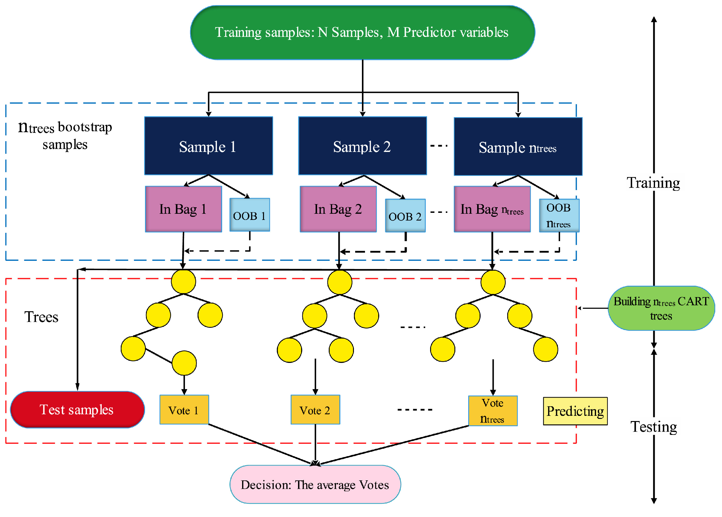
2.2. Random Forest (RF) Algorithm

The RF model was first presented by Breiman (2000) as a successful learning method that uses a collection of decision trees. RF are typically categorized into two primary applications: regression and classification. The suggested approach is created by combining decision trees that are produced from random bootstrap samples of the input datasets [38]. RF can improve model accuracy and reduce the chance of overfitting as compared to individual regression trees [38,39].
Essentially, the RF algorithm requires two crucial parameters to be set for its execution: the number of trees (n_estimators) to be generated and the number of predictor (feature) variables (max_features) to be employed for model tuning [39]. As illustrated in Figure 2, the primary steps in constructing an RF model are described as follows:
Step 1: Determine the number of trees (n_estimators) to be included in the RF.
Step 2: Create bootstrap samples by drawing n_estimators instances with replacement from the training dataset to train individual trees.
Step 3: Select predictors (max_features) by randomly choosing a subset of p predictors at each node to identify the best split point.
Step 4: Identify the optimal split by finding the best predictor and split point among the selected predictors, then divide the node into two sub-nodes.
Step 5: Make predictions by aggregating the outputs of all trees, averaging their predictions for regression or applying majority voting for classification.
Typically, the RF constructs numerous arbitrary binary trees to produce a forest. For this procedure, a bootstrap subset is employed to develop the individual tree. To achieve this, it applies the Classification and Regression Trees (CART) approach with the random variables selected at each node [40,41]. Subsequently, the ’out-of-bag’ procedure (OOB) is calculated using the learning data set which is not utilized in a bootstrap subset. In fact, the OOB refers to an error rate applied to assess the estimation error of ML algorithms like RF. Furthermore, the introduced error technique is used to validate the performance of an RF and to select optimal configurations for the hyperparameters to be tuned, such as the number of predictors [42]. Therefore, to decrease the out-of-bag (OOB) error and develop a RF model with peak performance, it is vital to fine-tune the two primary parameters: the total number of trees and the number of predictors used [40,43]. The following part will demonstrate the hyperparameter tuning methodology in depth and clarify its function in optimizing the accuracy of the RF predictor.

2.3. Hyperparameter Tunning Methodology

To prevent overfitting, Random Forest (RF) must be carefully adjusted. Since tuning hyperparameters in the machine learning algorithm can greatly affect its prediction accuracy, it is important to choose the right hyperparameters. The common method for hyperparameter tuning is using Grid Search. Researchers can adjust two hyperparameters in RF to manage the model’s uncertainty:
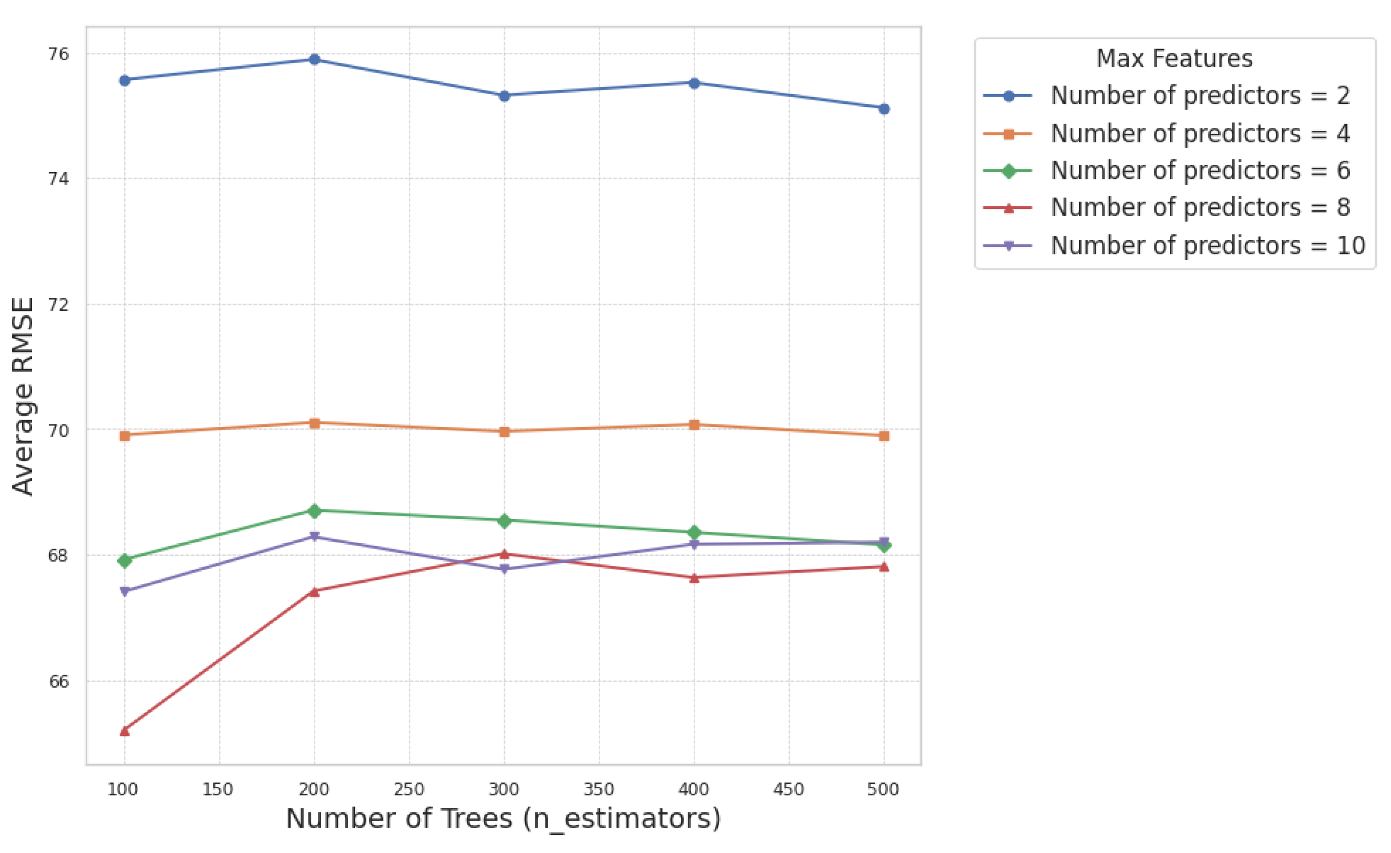
  • Number of trees (n_estimators): This indicates the number of decision trees present in the forest. While increasing the number of trees can improve model performance, an excessively high value may lead to overfitting.
  • Number of variables randomly selected at each split (Max_features): This determines how many features are considered when creating splits in the decision trees.
In this study, we fine-tuned the mtry and ntree parameters to enhance the RF prediction model’s performance. We utilized grid search and cross-validation (CV) techniques to assess different hyperparameter combinations. By methodically navigating the parameter space, grid search pinpoints the best configurations for the model. Each grid axis denotes an RF parameter, with every point representing a distinct set of parameter values. The optimization process assesses model performance at each grid point. To ensure robust model evaluation, we used k-fold CV during the hyperparameter tuning process. K-fold CV is one of the most popular validation methods in ML, providing a balance between bias and variance. Although there are no strict rules for choosing the number of folds (k), values of 5 or 10 are commonly used. Research [44] suggests that implementing 5 or 10 folds reduces the bias in estimating performance. In this research, we chose k = 5, executing ten rounds of training and validation using different subsets of data. The outcomes from these rounds were averaged to illustrate the RF model’s efficiency on the training dataset. All data processing tasks in this study were carried out using scikit-learn (sklearn). The library was utilized for model implementation, hyperparameter tuning, and validation, ensuring a robust and reliable evaluation of the RF model’s performance. The final hyperparameter tunning procedure is illustrated in Figure 3.

2.4. Feature Importance (Shapley Method)

Lundberg and Lee [45], inspired by game theory, applied Shapley’s concept of Shapley values to ML, resulting in the development of the SHAP technique. The game-theory-based SHAP approach has been widely adopted in recent years to create explanatory models for ML techniques, producing positive outcomes across various domains [45,46,47]. For instance, Mangalathu et al. [46] applied SHAP to analyze the failure modes and effects of reinforced concrete (RC) members, providing insights into the contribution of different structural parameters to failure prediction. Somala et al. [47] utilized SHAP to interpret machine learning models for predicting peak ground velocity (PGV) and peak ground acceleration (PGA) in seismic studies, enhancing the transparency of model predictions in geotechnical applications.The core idea of the SHAP method is to use Shapley values of sample feature values to evaluate the impact of input parameters. This approach not only explains the results of individual samples but also determines the overall influence of features at the dataset level. Since all features are regarded as contributors in SHAP’s additive feature attribute technique, the output objective is specified as a linear addition of the input features, which can be expressed as:
f ( x ) = g ( x ) = ϕ 0 + i = 1 M ϕ i x i
where  f ( x )  represents the original ML model that predicts an output based on the input features x, and  g ( x )  is a simplified surrogate model used for interpretation.  ϕ 0  is the baseline or expected value of the model’s prediction when no input features are present, and  ϕ i  represents the Shapley value for the i-th feature, quantifying its contribution to the prediction. Finally,  x i  is a binary indicator showing whether the i-th feature is included in the simplified model.
The SHAP approach serves as a tool for interpreting ML models, providing a means to examine and comprehend the complex operations of black-box model training. When used with ML models, SHAP allocates weights to features in each sample from the training data, performs a weighted fit to assess the importance of each feature (denoted by  ϕ i ), and defines a reference value. This reference value is then merged with the contributions from individual input features to compute the expected results of the ML models. After conducting the SHAP analysis, the baseline value—unaffected by any feature contributions—is regarded as the average predicted outcome.

2.5. Performance Metrics

To evaluate the performance of the models, the correlation coefficient ( R 2 ), MAE, RMSE, and MAPE metrics are employed [48]. The coefficient of determination  R 2  , calculates how reliably the predictions of a model align with the real values. A larger  R 2  score suggests that the algorithm explains a larger proportion of the variance in the target variable. RMSE indicates the average error magnitude between actual and predicted values, emphasizing larger errors more than smaller ones and giving an idea of the error scale. MAE calculates the mean of absolute discrepancies between predictions and observed values, offering a straightforward measure of prediction accuracy, valuable for understanding error sizes in relation to actual values. Ideally, a model should display lower MAE and RMSE values alongside higher  R 2  scores. The statistical metrics are outlined below:
Correlation of determination ( R 2 ):
R 2 = 1 ( y true y pred ) 2 ( y true y mean ) 2
Mean absolute error (MAE):
MAE = 1 n y true y pred
Root Mean Square Error (RMSE):
RMSE = 1 n ( y true y pred ) 2
where  y true  represents the actual values,  y pred  denotes the predicted values, and  y mean  is the mean of the actual values.

3. Database Used

The independent and dependent variables (Table 1) are examined to model the project cost for energy plants in Bangladesh [30]. The project-relevant variables are Contingency in construction cost, plant type based on the power generation mechanism, construction cost, type of contract under which the project is constructed, location of the power plant, and the power generation capacity of the plant; and the economic indicators include construction GDP, inflation rate, owner organization of the power plant, and total gross domestic product (GDP) of the country.
Three sources were used to collect project-related data: (1) access the web pages of the Bangladesh Power Development Board (BPDB), Northwest Power Company Limited (NWPCL), and Ashuganj Power Company Limited (APCL); (2) analysis of project records; and (3) specialist assessment. Information related to type of contract (Engineering, Procurement and Construction (EPC), Build-Own-Own-Operate (BOO), and Turn-Key), plant ownership (BPDB, NWPCL, APCL, etc.), power generation capacity (Megawatt), type of plant (Combined Cycle Power Plant (CCPP), Heavy Fuel Oil (HFO), Coal and Natural Gas), construction year, location (urban, peri-urban, and rural), and estimated cost for the projects are obtained from the web pages of the associated entities.
Among the 58 projects considered, the oldest project was built in 1993, whereas the most recent initiated in 2020. The mean project cost is about USD 290 million, whereas the mean power output potential is about 258 MW. Each of the ten categorical variables was further divided into binary variables. The proportion allocation of the projects with respect to binary variables related to ownership, plant type, type of contract, and project location are as follows: 57% are CCPP, 43% are owned by the BPDB, and 76% were awarded through EPC contracts. Additionally, 53% of the projects are in rural areas, 40% in peri-urban areas, and the remainder in urban areas.

4. Model Results

4.1. Hyperparameter Tunning Results

Figure 4 illustrates the relationship between the number of trees (n_estimators) and the average RMSE across different values of the maximum number of features (max_features). The plot demonstrates that the model’s performance is sensitive to both parameters, with the average RMSE showing variation as max_features changes. Notably, the lowest RMSE is observed for max_features = 8 when the number of trees exceeds 100, indicating an ideal balance between the number of predictors and model complexity.
The plot also reveals that as the number of trees increases, the RMSE tends to stabilize for most values of max_features. For instance, when max_features = 2, the RMSE remains relatively high across all values of n_estimators, suggesting that using fewer predictors leads to less effective splits in the RF model. On the other hand, for higher values of max_features (e.g., max_features = 8 and max_features = 10), the RMSE decreases and stabilizes more rapidly with increasing n_estimators, reflecting the benefit of including more predictors during split decisions.
Based on the visualization, the optimal settings for the RF model appear to be n_estimators = 100 and max_features = 8, where the RMSE achieves its lowest value. These settings ensure a good trade-off between model accuracy and computational efficiency. The corresponding RMSE,  R 2 , and MAE values for the optimal configuration are 65.19, 0.75, and 51.41, respectively, indicating the model’s robustness and accuracy under these parameters.

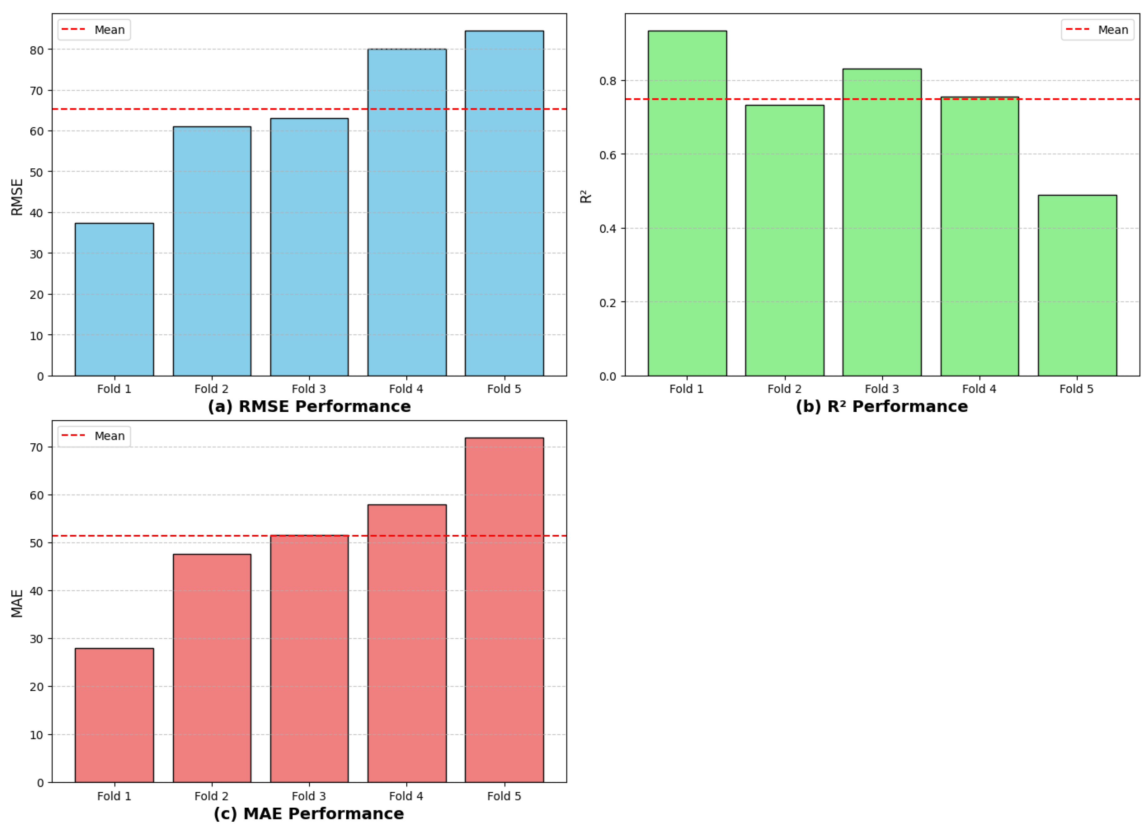
4.2. Optimal RF Model Five Fold Cross Validation Resutls

To test the robustness and generalization of our model, five folds cross validation technique is performed in our study. This technique reduce bias that can occur from random sampling by dividing the dataset into five equal folds. One fold is used for validation, on other hand the remaining four are used for training the model in each iteration. This process is repeated five times and each fold acting as the validation set once. After all five iterations, the overall model performance is calculated. Cross validation is well known for giving a robust estimate of model accuracy and stability.
Figure 5 and Table 2 illustrates the performance metrics—Root Mean Square Error (RMSE), coefficient of determination ( R 2 ), and Mean Absolute Error (MAE)—across the five folds. It is evident from the figure that there are variations in the model’s performance across different folds. Specifically, the RMSE values range from 37.416 to 84.486, with an average of 65.198 and a standard deviation of 16.670, indicating some fluctuations in error magnitude across the folds. The MAE follows a similar trend, with values ranging from 28.012 to 71.954, resulting in an average of 51.418 and a standard deviation of 14.331. These variations suggest that certain data partitions may be more challenging for the model to predict accurately.
In terms of  R 2 , the results demonstrate the model’s varying predictive power, with values ranging from a high of 0.933 in Fold 1 to a low of 0.489 in Fold 5. The mean  R 2  across all folds is 0.748, with a standard deviation of 0.147, which highlights the model’s overall moderate predictive strength. The relatively lower  R 2  in Fold 5 suggests that this subset may contain more complex or outlier data points, leading to decreased accuracy.
Despite the observed fluctuations, the model maintains a reasonable level of accuracy overall, as reflected in the mean values of the performance metrics. The relatively low standard deviations for RMSE and MAE indicate that the model is generally stable across different folds, albeit with room for improvement in achieving more consistent performance.

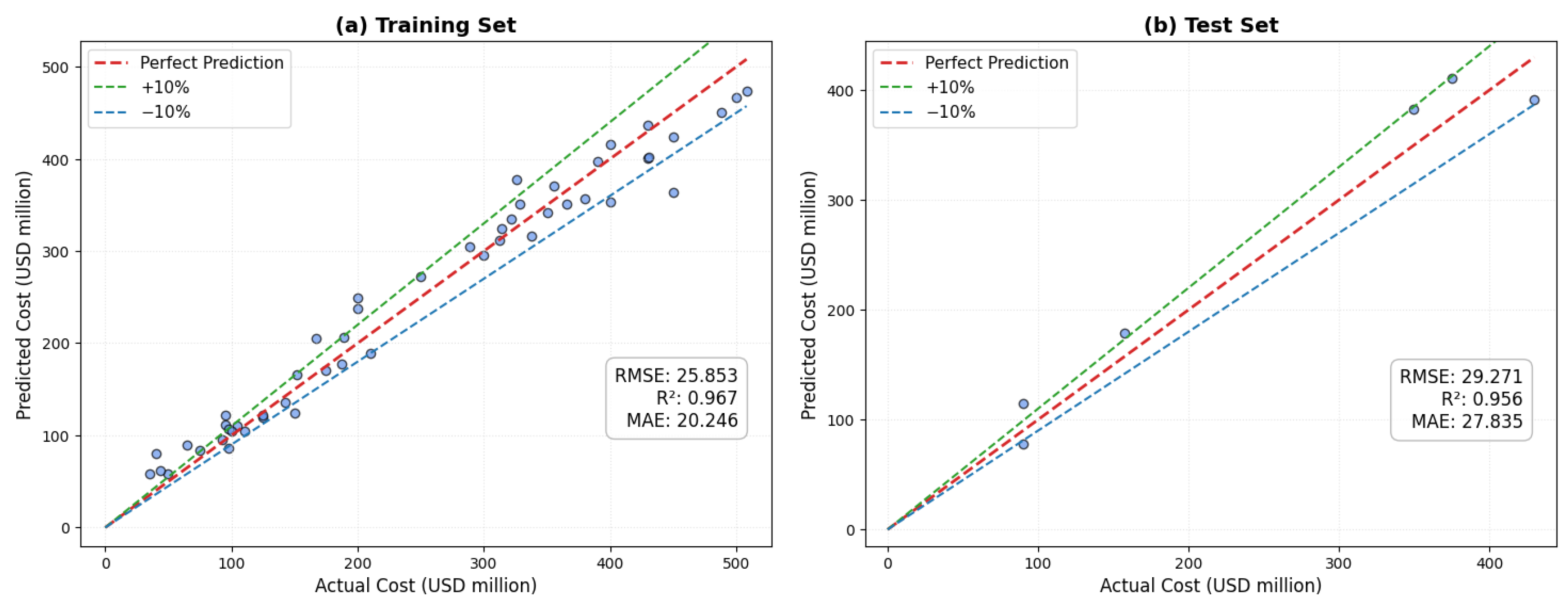
4.3. Model Performance Based on Training and Testing Sets

The prediction performance of the proposed model was evaluated after determining the optimal hyperparameters. The prediction results are presented in Figure 6, with the X and Y axes representing the actual and predicted project costs (USD million), respectively. The training and testing outcomes are illustrated in Figure 6a and Figure 6b, respectively, with data points represented by blue dots. The red dashed line indicates perfect prediction, while the green and blue dashed lines correspond to a ±10% margin of error.
In the training set (Figure 6a), most predicted values closely align with the actual costs, demonstrating high accuracy. The RMSE, MAE, and  R 2  for the training set were 25.853, 20.246, and 0.967, respectively. Similarly, the testing set (Figure 6b) shows good agreement between predicted and actual costs, with performance metrics of RMSE = 29.271, MAE = 27.835, and  R 2  = 0.956. These metrics indicate that the model generalizes well to unseen data, with only minor deviations from the perfect prediction line.
In both subplots, the majority of predictions fall within the ±10% tolerance band, further emphasizing the model’s reliability. The results suggest that the proposed approach effectively captures the underlying patterns in the data and can be considered a robust tool for estimating power plant construction costs.

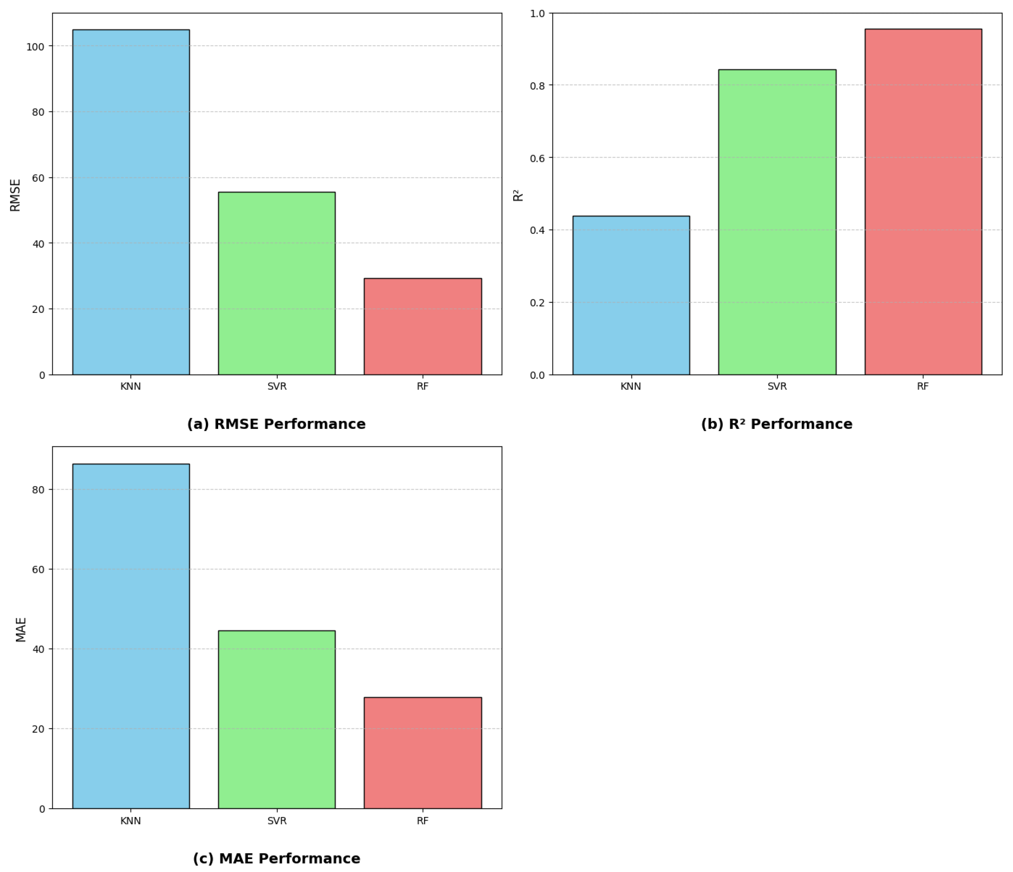
4.4. Performance Comparison with Single Learner ML Model

To better evaluate the performance of the RF model, comparisons are made with two widely used ML methods: Support Vector Regression (SVR) and K-Nearest Neighbors (KNN), based on the test set results. The hyperparameters for each model were optimized through grid search to ensure fair comparisons. The performance results for the three models are illustrated in Figure 7 and summarized in Table 3.
The plots in Figure 7 demonstrate that the RF model achieves significantly better prediction performance compared to SVR and KNN on the test set. Figure 7a highlights that the RMSE for RF is the lowest at 29.27, compared to 55.61 for SVR and 104.87 for KNN, indicating that RF predictions are much closer to the actual values. Similarly, Figure 7c shows that the MAE for RF is 27.83, outperforming SVR (44.60) and KNN (86.37), further affirming its superior predictive accuracy. The  R 2  values in Figure 7b also reflect this trend, with RF achieving 0.956, a notable improvement over SVR (0.842) and KNN (0.439), indicating RF’s higher ability to explain the variance in the data.
The improvement percentages further highlight RF’s advantage on the test set. The  R 2  improvement from SVR to RF is approximately 11.94%, showcasing RF’s superior explanatory power. For RMSE, the improvement from SVR to RF is approximately 90.01%, indicating a substantial reduction in prediction error. Similarly, the improvement in MAE is approximately 60.21%, emphasizing RF’s enhanced accuracy in minimizing absolute prediction errors.
The superior performance of the RF model can be attributed to its ensemble learning nature, which combines multiple decision trees to minimize errors and improve robustness. In contrast, SVR and KNN are individual learning algorithms and do not benefit from the collective decision-making of ensemble methods. As shown in Table 3, the RF model consistently outperforms both SVR and KNN across all metrics on the test set, similar to findings reported in prior studies. These results confirm that ensemble learning methods like RF are more suitable for predicting power plant construction costs compared to single learning algorithms like SVR and KNN.

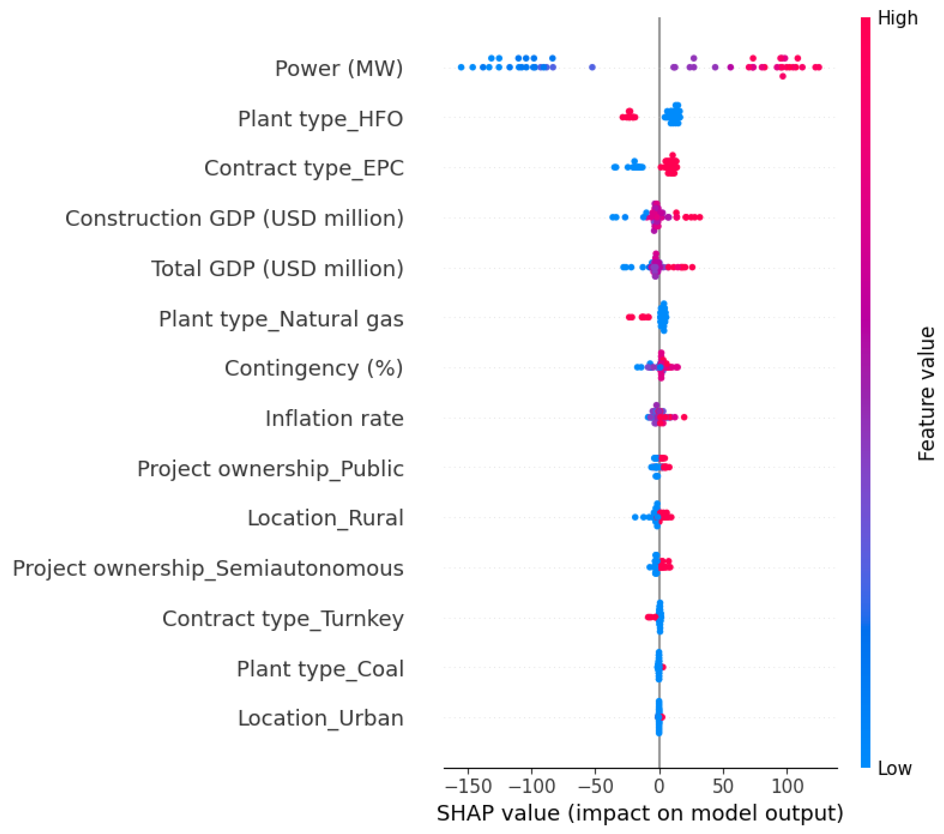
4.5. Feature Importance and SHAP Value

Figure 8 illustrates the global feature importance derived from the SHAP (SHapley Additive exPlanations) values for the RF model used to predict construction costs. The horizontal bars represent the mean absolute SHAP value for each feature, indicating the contribution of each variable to the model’s predictions. The features are ranked in descending order of importance based on their average impact on the predictions.
According to the figure, the variable Power (MW) has the highest mean SHAP value ( + 95.01 ), indicating it is the most influential feature in predicting construction costs. This is followed by Plant type_HFO ( + 10.68 ), which refers to Heavy Fuel Oil power plants, and Contract type_EPC ( + 9.41 ), which represents the Engineering, Procurement, and Construction contract type. These variables also contribute significantly to the model’s performance. Other important variables include Construction GDP (USD million) ( + 7.31 ) and Total GDP (USD million) ( + 5.97 ), which capture economic factors associated with the construction year.
Lower-ranked features such as Contingency (%) ( + 4.29 ), Inflation rate ( + 3.84 ), and Location_Rural ( + 2.90 ) exhibit less impact, while the Sum of 5 other features collectively contributes a mean SHAP value of ( + 6.97 ).
Figure 8 highlights the critical role of Power (MW) in influencing construction costs, underscoring its dominant contribution to the model. Heavy Fuel Oil plant type and the use of Engineering, Procurement, and Construction contracts also emerge as significant determinants. One limitation of this global importance plot is that it provides an averaged view of feature influence but does not capture the specific direction (positive or negative) of the impact for individual predictions. Despite this limitation, the SHAP analysis offers valuable insights into the key variables driving the model’s predictions, emphasizing the importance of Power (MW) and other high-ranking features in understanding construction cost variability.
The SHAP summary plot shown above provides a comprehensive understanding of feature importance and their direction of impact on the construction cost prediction. The plot is generated using the SHAP tree explainer algorithm, which combines local explanations to interpret the behavior of ensemble tree-based ML models across the dataset. In this plot, each dot represents an individual data point, with the position of the dots on the x-axis indicating the SHAP value, or the impact of the respective feature values on the predicted cost. The y-axis lists the features ranked in descending order of importance, with the most influential features appearing at the top. The color of the dots represents the feature value, with red indicating high feature values and blue indicating low feature values.
Figure 9 reveals that Power (MW) is the most critical factor affecting the construction cost, as evidenced by its wide spread of SHAP values. Higher power capacities, represented by red dots on the right side of the x-axis, correspond to greater positive impacts on construction costs, whereas lower capacities (blue dots) tend to decrease costs. Similarly, Contract type_EPC has a significant impact, with higher SHAP values indicating that this contract type is generally associated with increased predicted costs. One interesting finding is that the Heavy Fuel Oil (HFO) plant type is associated with a reduction in the construction cost of power plants.
Other features such as Construction GDP (USD million) and Total GDP (USD million) also exhibit noticeable influence on cost predictions, with high feature values increasing the predicted costs. Conversely, variables like Location_Rural and Plant type_Coal show relatively lower importance, though their SHAP values suggest they still contribute to the model’s performance.

5. Conclusions

In this study, an innovative machine learning algorithms named as Random Forest (RF) was employed to estimate the construction costs of different parameters. Our model performed effectively in terms of precision and applicability. In this study, we used a diverse dataset that contained a total of 58 power plant projects. The data records were split into testing and training portions, with 10% of the data sets used for testing evaluation and the remaining 90% used for model training. Furthermore, the performance effectiveness of the our RF models was compared with two single learner models (SVR and KNN) employing three statistical measures. In addition, Shap analysis is utilized to evaluate the impact of the variables on construction costs.
  • The RF algorithm is closely aligned and adjacent to the perfect match line. In the RF model, most predictions are adjusted within the error margins ranging from +10% to −10%.
  • In the research, three quantitative metrics are applied to measure the capability of models. The RF model demonstrated the highest outstanding R-square scores, about 0.967 and 0.956, respectively, at the train and test phases. In comparison, the KNN and SVR models exhibited approximately 0.438 and 0.842 in the testing stage. Notably, the remaining numerical metrics similarly behave superior for the RF model compared to the KNN and SVR models.
  • The Shapley method implemented in this research revealed essential findings. The highly impactful attribute influencing overall construction cost estimates was determined as power (MW), followed by the heavy fuel oil (HFO) plant type, and the Contract type EPC. In particular, the study demonstrated that costs tend to increase when factors such as power (MW) and Contract type EPC increase, and decrease when the plant construction type is HFO.
This study’s dataset, comprising 58 power plant projects, is relatively small and may limit the generalizability of the findings. Future research should consider larger and more diverse datasets to validate the results. Additionally, exploring other ensemble methods such as Gradient Boosting Machines could provide a broader perspective on algorithm performance. Extending the analysis to incorporate real-time data and dynamic modeling could enhance the practical relevance of the findings.

Author Contributions

Conceptualization, S.F.M.A. and M.A.A.; methodology, M.A.A.; software, H.I.; validation, L.F.A.B. and H.A.S.P.; formal analysis, M.A.A. and S.F.M.A.; investigation, S.F.M.A.; resources, H.A.S.P.; data curation, M.A.A. and S.H.R.; writing—original draft preparation, S.F.M.A.; writing—review and editing, H.I., L.F.A.B., H.A.S.P., and S.H.R.; visualization, H.I. and S.H.R.; supervision, H.A.S.P. and L.F.A.B.; project administration, H.I.; funding acquisition, H.A.S.P. All authors have read and agreed to the published version of the manuscript.

Funding

This work was partially supported by the GeoBioTec Research Unit, through the strategic projects UIDB/04035/2020 (https://doi.org/10.54499/UIDB/04035/2020) and UIDP/04035/2020 (https://doi.org/10.54499/UIDP/04035/2020), funded by the Fundação para a Ciência e a Tecnologia, IP/MCTES through national funds (PIDDAC). Funding for the period 2025–2029—transition phase.

Data Availability Statement

The data presented in this study are available in [30].

Conflicts of Interest

The authors declare no conflicts of interest.

References

  1. Sovacool, B.K.; Gilbert, A.; Nugent, D. An international comparative assessment of construction cost overruns for electricity infrastructure. Energy Res. Soc. Sci. 2014, 3, 152–160. [Google Scholar] [CrossRef]
  2. IHS. IHS Costs and Strategic Sourcing: Power Capital Costs Index and European Power Capital Costs Index. Available online: https://www.ihs.com/info/cera/ihsindexes/index.html (accessed on 1 April 2025).
  3. Sovacool, B.K.; Nugent, D.; Gilbert, A. Construction cost overruns and electricity infrastructure: An unavoidable risk? Electr. J. 2014, 27, 112–120. [Google Scholar] [CrossRef]
  4. Kagiri, D.; Wainaina, G. Time and Cost Overruns in Power Projects in Kenya: A Case Study of Kenya Electricity Generating Company Limited. Orsea J. 2013, 3. [Google Scholar]
  5. Bouayed, Z. Using Monte Carlo simulation to mitigate the risk of project cost overruns. Int. J. Saf. Secur. Eng. 2016, 6, 293–300. [Google Scholar] [CrossRef]
  6. Khodeir, L.M.; El Ghandour, A. Examining the role of value management in controlling cost overrun [application on residential construction projects in Egypt]. Ain Shams Eng. J. 2019, 10, 471–479. [Google Scholar] [CrossRef]
  7. Love, P.E.; Sing, C.P.; Carey, B.; Kim, J.T. Estimating construction contingency: Accommodating the potential for cost overruns in road construction projects. J. Infrastruct. Syst. 2015, 21, 04014035. [Google Scholar] [CrossRef]
  8. Lin, H. An artificial neural network model for data prediction. Adv. Mater. Res. 2014, 971, 1521–1524. [Google Scholar] [CrossRef]
  9. Arafa, M.; Alqedra, M. Early stage cost estimation of buildings construction projects using artificial neural networks. J. Artif. Intell. 2011, 4, 63–75. [Google Scholar] [CrossRef]
  10. Sodikov, J. Cost estimation of highway projects in developing countries: Artificial neural network approach. J. East. Asia Soc. Transp. Stud. 2005, 6, 1036–1047. [Google Scholar]
  11. Ahiaga-Dagbui, D.D.; Smith, S.D. Neural networks for modelling the final target cost of water projects. In Proceedings of the 28th Annual ARCOM Conference, Edinburgh, UK, 3–5 September 2012; Smith, S.D., Ed.; Association of Researchers in Construction Management: Edinburgh, UK, 2012; pp. 307–316. [Google Scholar]
  12. Khashei, M.; Bijari, M. An artificial neural network (p, d, q) model for timeseries forecasting. Expert Syst. Appl. 2010, 37, 479–489. [Google Scholar] [CrossRef]
  13. Ali, Z.H.; Burhan, A.M. Hybrid machine learning approach for construction cost estimation: An evaluation of extreme gradient boosting model. Asian J. Civ. Eng. 2023, 24, 2427–2442. [Google Scholar] [CrossRef]
  14. Chakraborty, D.; Elhegazy, H.; Elzarka, H.; Gutierrez, L. A novel construction cost prediction model using hybrid natural and light gradient boosting. Adv. Eng. Inform. 2020, 46, 101201. [Google Scholar] [CrossRef]
  15. Jin, R.; Cho, K.; Hyun, C.; Son, M. MRA-based revised CBR model for cost prediction in the early stage of construction projects. Expert Syst. Appl. 2012, 39, 5214–5222. [Google Scholar] [CrossRef]
  16. Lu, Y.; Luo, X.; Zhang, H. A gene expression programming algorithm for highway construction cost prediction problems. J. Transp. Syst. Eng. Inf. Technol. 2011, 11, 85–92. [Google Scholar] [CrossRef]
  17. Tayefeh Hashemi, S.; Ebadati, O.M.; Kaur, H. Cost estimation and prediction in construction projects: A systematic review on machine learning techniques. SN Appl. Sci. 2020, 2, 1703. [Google Scholar] [CrossRef]
  18. Wang, J.; Ashuri, B. Predicting ENR construction cost index using machine-learning algorithms. Int. J. Constr. Educ. Res. 2017, 13, 47–63. [Google Scholar] [CrossRef]
  19. Zhao, L.; Zhang, W.; Wang, W. Construction cost prediction based on genetic algorithm and BIM. Int. J. Pattern Recognit. Artif. Intell. 2020, 34, 2059026. [Google Scholar] [CrossRef]
  20. Tijanić, K.; Car-Pušić, D.; Šperac, M. Cost estimation in road construction using artificial neural network. Neural Comput. Appl. 2020, 32, 9343–9355. [Google Scholar] [CrossRef]
  21. Jiang, Q. Estimation of construction project building cost by back-propagation neural network. J. Eng. Des. Technol. 2020, 18, 601–609. [Google Scholar] [CrossRef]
  22. Wang, X. Application of fuzzy math in cost estimation of construction project. J. Discret. Math. Sci. Cryptogr. 2017, 20, 805–816. [Google Scholar] [CrossRef]
  23. Swei, O.; Gregory, J.; Kirchain, R. Construction cost estimation: A parametric approach for better estimates of expected cost and variation. Transp. Res. Part B Methodol. 2017, 101, 295–305. [Google Scholar]
  24. Coffie, G.; Cudjoe, S. Using extreme gradient boosting (XGBoost) machine learning to predict construction cost overruns. Int. J. Constr. Manag. 2024, 24, 1742–1750. [Google Scholar] [CrossRef]
  25. Yan, H.; He, Z.; Gao, C.; Xie, M.; Sheng, H.; Chen, H. Investment estimation of prefabricated concrete buildings based on XGBoost machine learning algorithm. Adv. Eng. Informatics 2022, 54, 101789. [Google Scholar]
  26. El-Sawalhi, N.I. Support vector machine cost estimation model for road projects. J. Civ. Eng. Archit. 2015, 9, 1115–1125. [Google Scholar]
  27. Hashemi, S.T.; Ebadati E, O.M.; Kaur, H. A hybrid conceptual cost estimating model using ANN and GA for power plant projects. Neural Comput. Appl. 2019, 31, 2143–2154. [Google Scholar]
  28. Lee, J.G.; Lee, H.S.; Park, M.; Seo, J. Early-stage cost estimation model for power generation project with limited historical data. Eng. Constr. Archit. Manag. 2022, 29, 2599–2614. [Google Scholar]
  29. Islam, M.S.; Mohandes, S.R.; Mahdiyar, A.; Fallahpour, A.; Olanipekun, A.O. A coupled genetic programming Monte Carlo simulation–based model for cost overrun prediction of thermal power plant projects. J. Constr. Eng. Manag. 2022, 148, 04022073. [Google Scholar]
  30. Arifuzzaman, M.; Gazder, U.; Islam, M.S.; Skitmore, M. Budget and cost contingency CART models for power plant projects. J. Civ. Eng. Manag. 2022, 28, 680–695. [Google Scholar]
  31. Wang, F.; Ma, S.; Wang, H.; Li, Y.; Qin, Z.; Zhang, J. A hybrid model integrating improved flower pollination algorithm-based feature selection and improved random forest for NOX emission estimation of coal-fired power plants. Measurement 2018, 125, 303–312. [Google Scholar]
  32. Janoušek, J.; Gajdoš, P.; Dohnálek, P.; Radeckỳ, M. Towards power plant output modelling and optimization using parallel Regression Random Forest. Swarm Evol. Comput. 2016, 26, 50–55. [Google Scholar] [CrossRef]
  33. Tohry, A.; Chelgani, S.C.; Matin, S.; Noormohammadi, M. Power-draw prediction by random forest based on operating parameters for an industrial ball mill. Adv. Powder Technol. 2020, 31, 967–972. [Google Scholar] [CrossRef]
  34. Sessa, V.; Assoumou, E.; Bossy, M.; Simões, S.G. Analyzing the applicability of random forest-based models for the forecast of run-of-river hydropower generation. Clean Technol. 2021, 3, 858–880. [Google Scholar] [CrossRef]
  35. Guo, J.; Zan, X.; Wang, L.; Lei, L.; Ou, C.; Bai, S. A random forest regression with Bayesian optimization-based method for fatigue strength prediction of ferrous alloys. Eng. Fract. Mech. 2023, 293, 109714. [Google Scholar]
  36. Gupta, A.; Gowda, S.; Tiwari, A.; Gupta, A.K. XGBoost-SHAP framework for asphalt pavement condition evaluation. Constr. Build. Mater. 2024, 426, 136182. [Google Scholar] [CrossRef]
  37. Arslan, Y.; Lebichot, B.; Allix, K.; Veiber, L.; Lefebvre, C.; Boytsov, A.; Goujon, A.; Bissyandé, T.F.; Klein, J. Towards refined classifications driven by shap explanations. In Proceedings of the International Cross-Domain Conference for Machine Learning and Knowledge Extraction, Vienna, Austria, 23–26 August 2022; Springer: Berlin/Heidelberg, Germany, 2022; pp. 68–81. [Google Scholar]
  38. Breiman, L. Random forests. Mach. Learn. 2001, 45, 5–32. [Google Scholar] [CrossRef]
  39. Ho, T.K. Random decision forests. In Proceedings of the 3rd International Conference on Document Analysis and Recognition, Montreal, QC, Canada, 14–16 August 1995; IEEE: Piscataway, NJ, USA, 1995; Volume 1, pp. 278–282. [Google Scholar]
  40. Vorpahl, P.; Elsenbeer, H.; Märker, M.; Schröder, B. How can statistical models help to determine driving factors of landslides? Ecol. Model. 2012, 239, 27–39. [Google Scholar]
  41. Pourghasemi, H.R.; Kerle, N. Random forests and evidential belief function-based landslide susceptibility assessment in Western Mazandaran Province, Iran. Environ. Earth Sci. 2016, 75, 185. [Google Scholar] [CrossRef]
  42. Rahmati, O.; Pourghasemi, H.R.; Melesse, A.M. Application of GIS-based data driven random forest and maximum entropy models for groundwater potential mapping: A case study at Mehran Region, Iran. Catena 2016, 137, 360–372. [Google Scholar]
  43. Nicodemus, K.K.; Malley, J.D. Predictor correlation impacts machine learning algorithms: Implications for genomic studies. Bioinformatics 2009, 25, 1884–1890. [Google Scholar] [CrossRef]
  44. Rodriguez, J.D.; Perez, A.; Lozano, J.A. Sensitivity analysis of k-fold cross validation in prediction error estimation. IEEE Trans. Pattern Anal. Mach. Intell. 2009, 32, 569–575. [Google Scholar]
  45. Lundberg, S. A unified approach to interpreting model predictions. arXiv 2017, arXiv:1705.07874. [Google Scholar]
  46. Mangalathu, S.; Hwang, S.H.; Jeon, J.S. Failure mode and effects analysis of RC members based on machine-learning-based SHapley Additive exPlanations (SHAP) approach. Eng. Struct. 2020, 219, 110927. [Google Scholar]
  47. Somala, S.N.; Chanda, S.; Karthikeyan, K.; Mangalathu, S. Explainable Machine learning on New Zealand strong motion for PGV and PGA. Structures 2021, 34, 4977–4985. [Google Scholar]
  48. Jia, H.; Qiao, G.; Han, P. Machine learning algorithms in the environmental corrosion evaluation of reinforced concrete structures—A review. Cem. Concr. Compos. 2022, 133, 104725. [Google Scholar]
Figure 1. Methodological Framework for Predicting Power Plant Construction Costs Using the RF Algorithm.
Civileng 06 00021 g001
Figure 2. Workflow of the RF algorithm for construction cost prediction.
Civileng 06 00021 g002
Figure 3. Hyperparameter tuning process for RF using grid search with cross-validation.
Civileng 06 00021 g003
Figure 4. Impact of the number of trees and predictors on average RMSE in a RF model.
Civileng 06 00021 g004
Figure 5. Evaluation of model performance metrics across 5-fold cross-validation: (a) RMSE, (b R 2 , and (c) MAE.
Civileng 06 00021 g005
Figure 6. Actual vs. predicted construction costs with ±10% error margins during: (a) training; (b) testing phases.
Civileng 06 00021 g006
Figure 7. Performance comparison of KNN, SVR, and RF models on the test set: (a) RMSE, (b R 2 , and (c) MAE.
Civileng 06 00021 g007
Figure 8. Feature Importance Analysis Using SHAP Values: Highlighting the Key Drivers for Power Plant Costs.
Civileng 06 00021 g008
Figure 9. SHAP global explanation on RF model.
Civileng 06 00021 g009
Table 1. Description of Variables in the Power Plant Dataset.
Characteristic TypeVariableDescriptionType
Economic VariablesGDPTotal Bangladesh GDP during the construction year of the project.Integer (USD million)
Const. GDPGDP contribution of the construction sector in the construction year.Integer (USD million)
IRInflation rate in Bangladesh for the construction year.Integer (percentage)
Project CharacteristicsCostTotal construction cost of the project.Integer (USD million)
Cont.Estimated contingency as a percentage of the project cost.Integer (percentage)
PowerPower generation capacity of the project.Integer (MW)
Location VariablesLocationLocation of the project (Urban, Rural, Peri-Urban).Categorical (3 types)
Ownership VariablesOwnerOwnership type (Government, IPP, Semi-autonomous).Categorical (3 types)
Plant SpecificationsPlantType of power plant (CCPP, Coal, HFO, Natural Gas).Categorical (4 types)
Contract VariablesContractType of construction contract (EPC, BOO, Turnkey).Categorical (3 types)
Table 2. Performance Measures for Each Fold.
FoldRoot Mean Square Error (RMSE) R 2 Mean Absolute Error (MAE)
Fold 137.4160.93328.012
Fold 261.0010.73247.587
Fold 362.9580.82951.588
Fold 480.1270.75557.951
Fold 584.4860.48971.954
Mean65.1980.74851.418
Std Deviation16.6700.14714.331
Table 3. Performance Comparison of Models on the Test Set.
Model R 2 RMSE (kN)MAE (kN)
KNN0.439104.8786.37
SVR0.84255.6144.60
RF0.95629.2727.83
Disclaimer/Publisher’s Note: The statements, opinions and data contained in all publications are solely those of the individual author(s) and contributor(s) and not of MDPI and/or the editor(s). MDPI and/or the editor(s) disclaim responsibility for any injury to people or property resulting from any ideas, methods, instructions or products referred to in the content.

