
Rethinking the Methods and Algorithms for Inner Speech Decoding and Making Them Reproducible


Abstract
1. Introduction
State-of-the-Art Literature
2. Materials and Methods
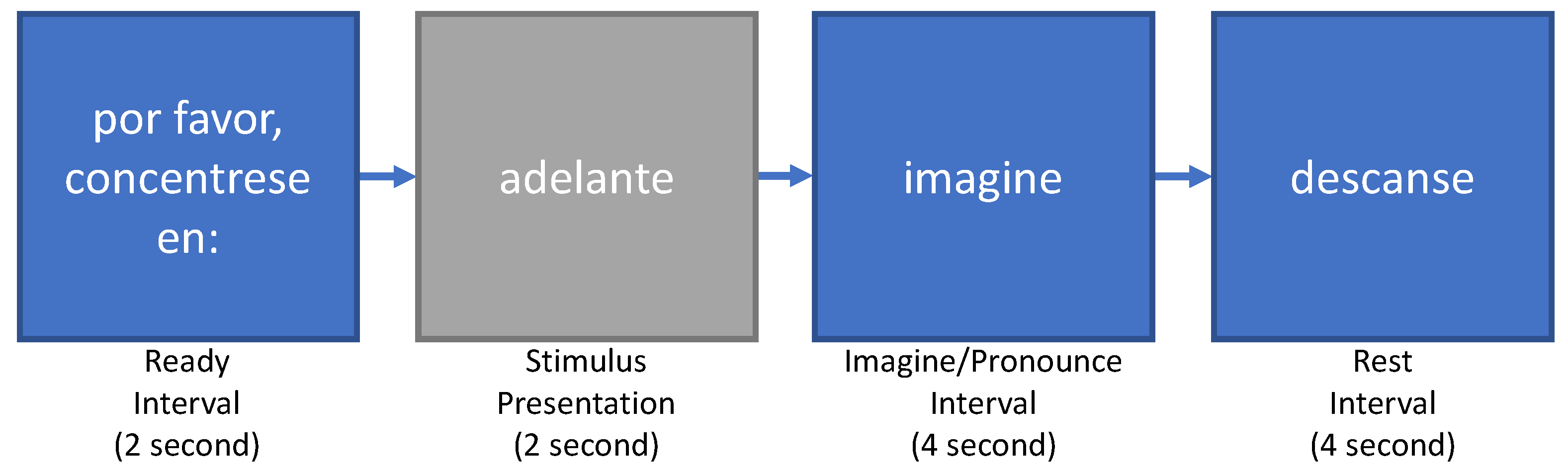
2.1. Dataset and Experimental Protocol
2.2. Methods
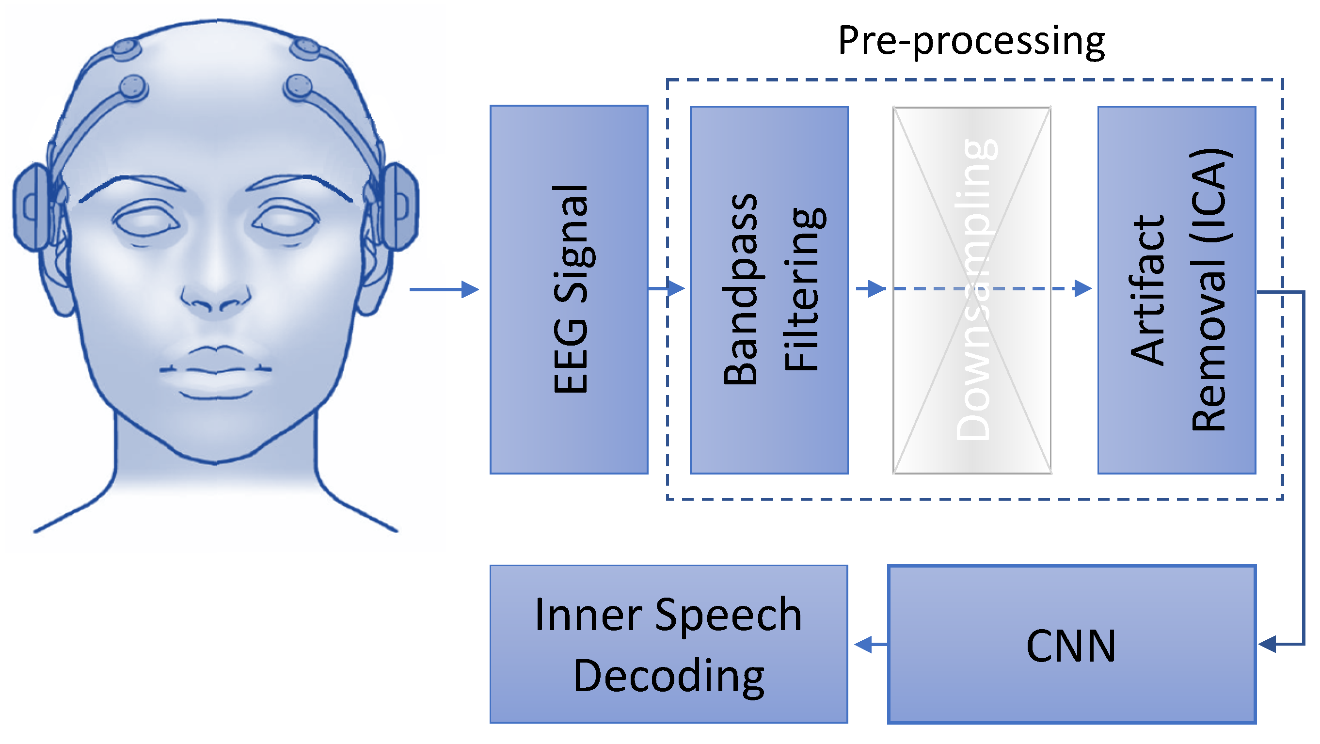
2.3. Preprocessing
- Filtering: A frequency between 2 Hz and 40 Hz is used for filtering [8].
- Down-sampling: The filtered data are down-sampled to 128 HZ. The original frequency of the data is 1024 Hz.
- Artifact removal: Independent component analysis (ICA) is known as a blind-source separation technique. When recording a multi-channel signal, the advantages of employing ICA become most obvious. ICA facilitates the extraction of independent components from mixed signals by transforming a multivariate random signal. Here, ICA applied to identify components in EEG signal that include artifacts such as eye blinks or eye movements. These are components then filtered out before the data are translated back from the source space to the sensor space. ICA effectively removes noise from the EEG data and is, therefore, an aid to classification. Given the small number of channels, we intact all the channels and instead use ICA [25] for artifact removal (https://github.com/pierreablin/picard/blob/master/matlab_octave/picard.m, accessed on 27 February 2022).
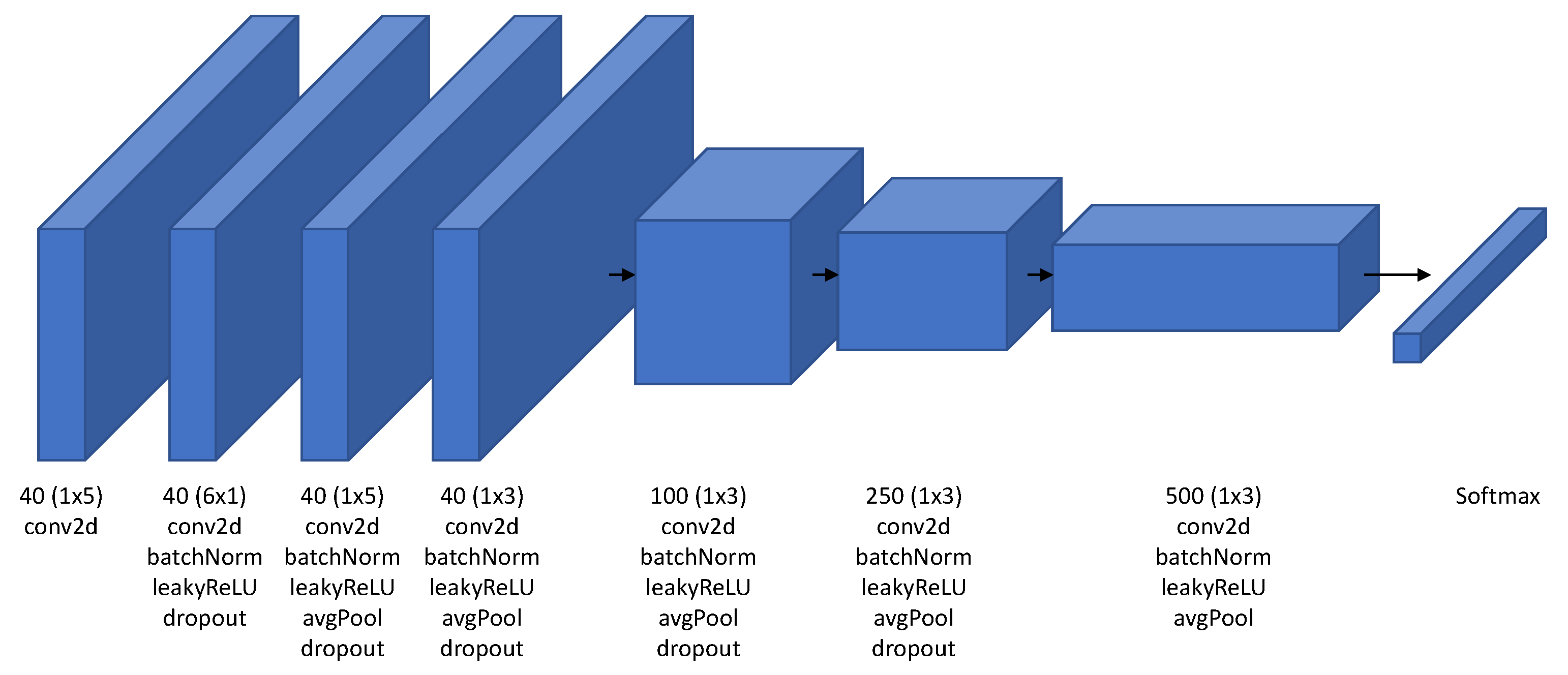
2.4. iSpeech-CNN Architecture
3. Experimental Approaches and Performance Measures
3.1. Experimental Approaches
3.1.1. Subject-Dependent/Within-Subject Approach
3.1.2. Subject Independent: Leave-One-Out Approach
3.1.3. Mixed Approach
3.2. Performance Measures
4. Results and Discussion: Vowels (Five Classes)
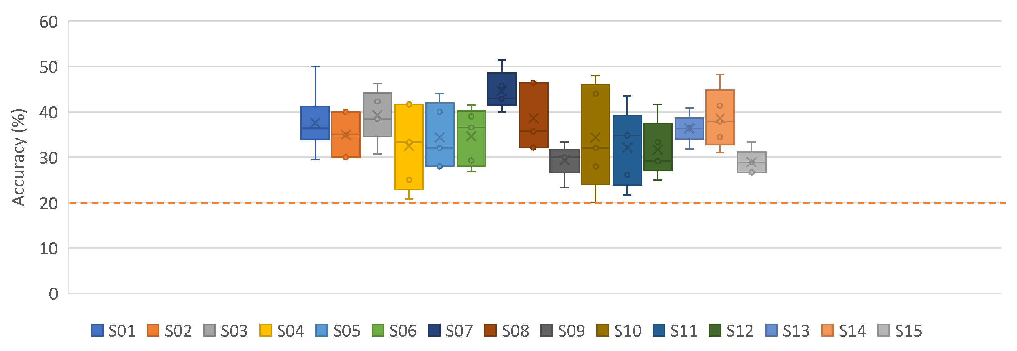
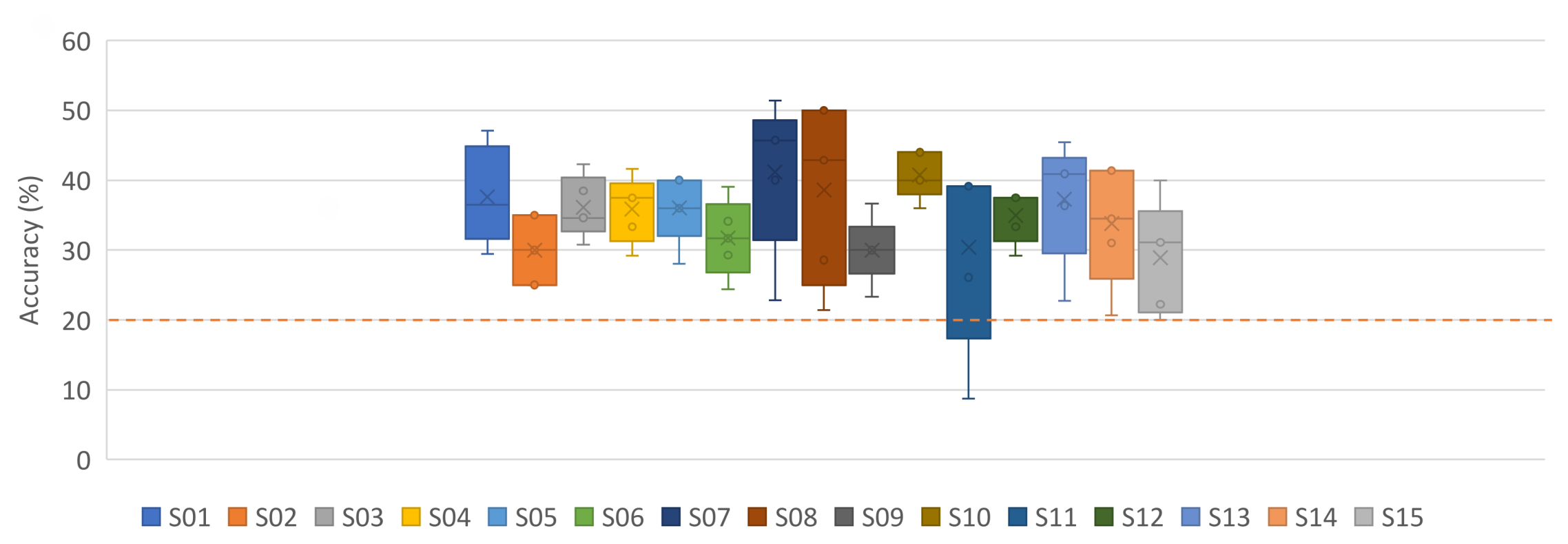
4.1. Subject-Dependent/Within-Subject Classification
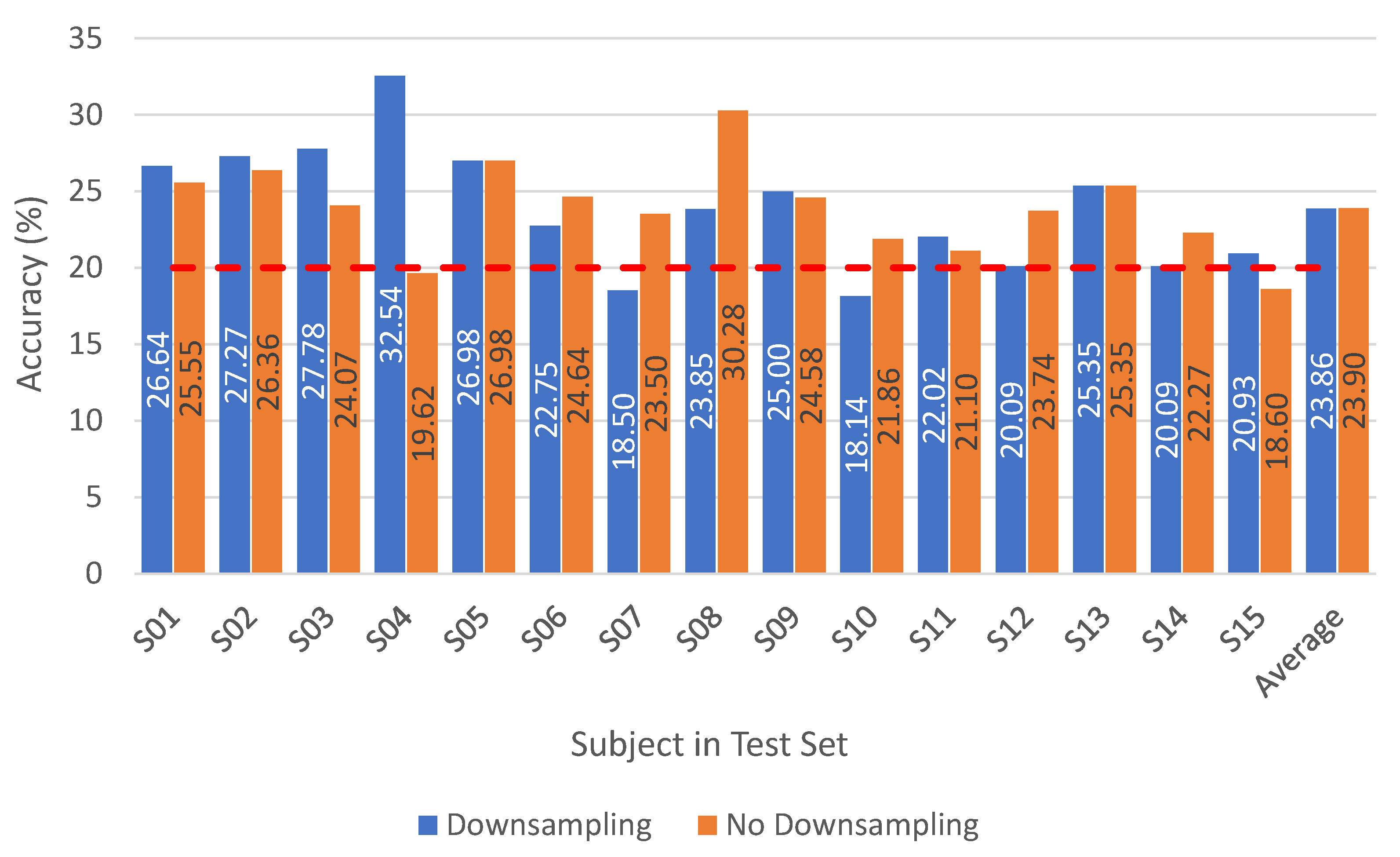
4.1.1. Ablation Study—Influence of Downsampling
4.1.2. Ablation Study—Influence of Preprocessing
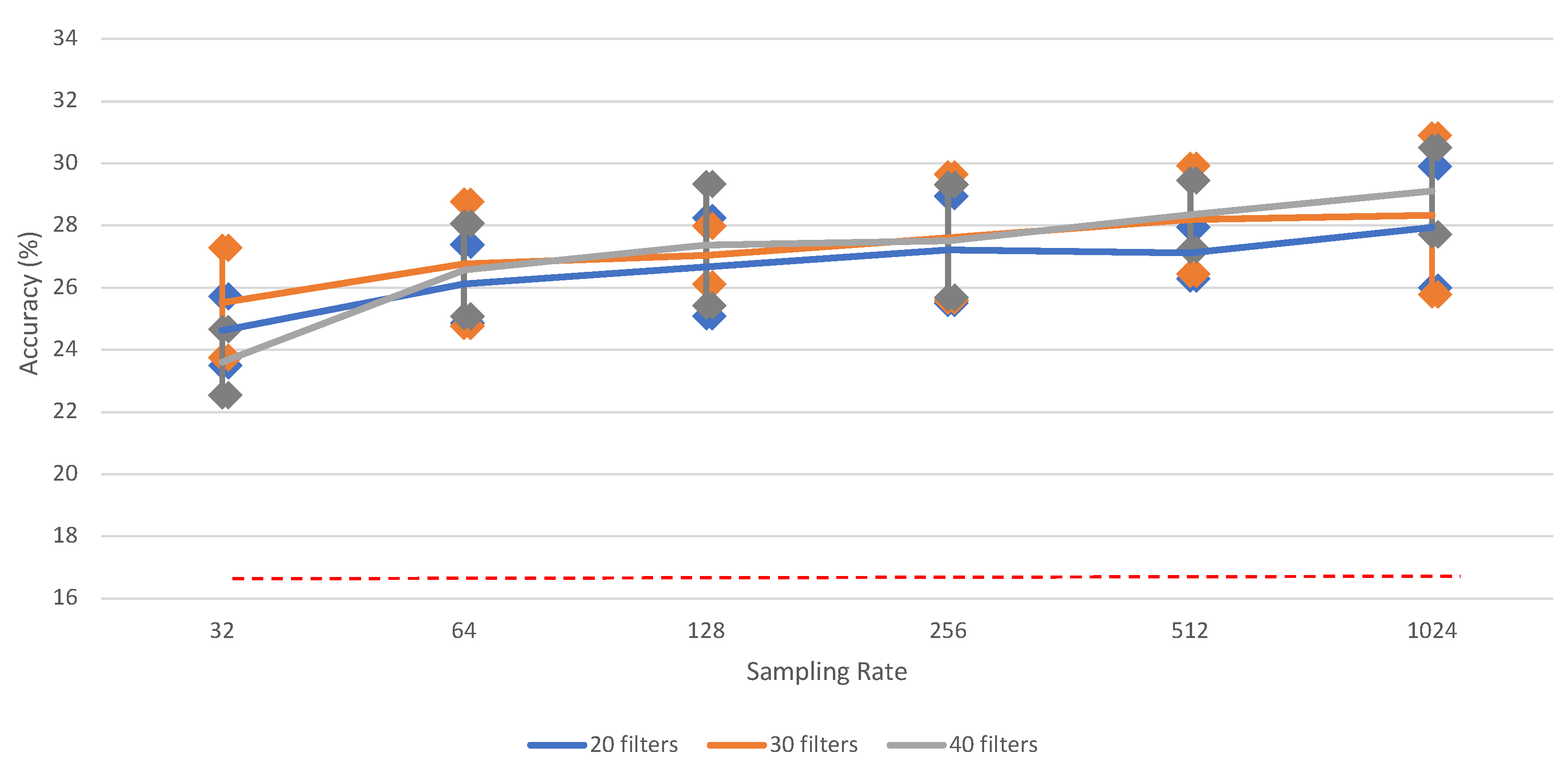
4.1.3. Ablation Study—Influence of Architecture
4.2. Mixed Approach Results
4.3. Subject-Independent: Leave-One-Out Results
5. Results and Discussion: Words (Six Classes)
6. Performance Comparison and Related Discussion
7. Conclusions
Author Contributions
Funding
Institutional Review Board Statement
Informed Consent Statement
Data Availability Statement
Conflicts of Interest
Appendix A. The Results on Vowels

| Raw | Downsampled | |||||
|---|---|---|---|---|---|---|
| Train | Validation | Test | Train | Validation | Test | |
| S01 | 91.07 | 36.00 | 35.29 | 79.07 | 39.20 | 26.47 |
| S02 | 92.44 | 29.00 | 17.00 | 72.00 | 24.00 | 16.00 |
| S03 | 83.65 | 34.00 | 27.69 | 86.94 | 26.00 | 19.23 |
| S04 | 89.94 | 38.00 | 33.33 | 89.33 | 30.00 | 31.67 |
| S05 | 86.59 | 16.00 | 21.60 | 72.82 | 19.00 | 17.60 |
| S06 | 91.73 | 27.00 | 25.85 | 80.00 | 29.00 | 27.80 |
| S07 | 95.17 | 31.00 | 26.86 | 85.66 | 33.00 | 28.00 |
| S08 | 88.12 | 29.00 | 21.43 | 83.06 | 24.00 | 21.43 |
| S09 | 83.89 | 35.20 | 30.00 | 82.38 | 30.40 | 26.00 |
| S10 | 88.35 | 29.00 | 20.80 | 63.88 | 26.00 | 19.20 |
| S11 | 80.91 | 25.00 | 22.61 | 86.06 | 23.00 | 16.52 |
| S12 | 88.57 | 29.00 | 26.67 | 96.23 | 37.00 | 30.83 |
| S13 | 80.00 | 38.00 | 29.09 | 93.94 | 36.00 | 31.82 |
| S14 | 79.66 | 27.20 | 22.76 | 73.49 | 27.20 | 23.45 |
| S15 | 83.20 | 23.00 | 20.00 | 91.73 | 28.00 | 20.89 |
| Average/Mean | 86.88 | 29.76 | 25.29 | 82.44 | 28.79 | 23.79 |
| Standard Deviation | 4.81 | 5.96 | 5.14 | 8.73 | 5.44 | 5.35 |
| Preprocessing (Filtering and Artifact Removal) | ||||||
|---|---|---|---|---|---|---|
| No Downsampling | Downsampling | |||||
| Train | Validation | Test | Train | Validation | Test | |
| S01 | 96.65 | 38.40 | 38.82 | 91.44 | 43.20 | 38.82 |
| S02 | 92.78 | 40.00 | 25.00 | 99.33 | 32.00 | 27.00 |
| S03 | 99.88 | 38.00 | 34.62 | 99.41 | 36.00 | 32.31 |
| S04 | 99.15 | 43.00 | 32.50 | 97.45 | 42.00 | 30.83 |
| S05 | 89.29 | 37.00 | 26.40 | 93.41 | 34.00 | 35.20 |
| S06 | 95.47 | 38.00 | 37.56 | 98.80 | 38.00 | 32.20 |
| S07 | 98.62 | 36.00 | 27.43 | 81.52 | 28.00 | 28.00 |
| S08 | 97.06 | 45.00 | 38.57 | 98.59 | 39.00 | 32.14 |
| S09 | 97.41 | 36.00 | 35.33 | 97.41 | 32.00 | 30.00 |
| S10 | 96.24 | 35.00 | 37.60 | 98.47 | 35.00 | 28.80 |
| S11 | 88.69 | 30.00 | 31.30 | 91.66 | 35.00 | 33.91 |
| S12 | 86.86 | 35.00 | 30.83 | 91.31 | 28.00 | 24.17 |
| S13 | 99.54 | 40.00 | 33.64 | 95.89 | 46.00 | 31.82 |
| S14 | 87.43 | 39.20 | 35.86 | 84.11 | 40.00 | 33.79 |
| S15 | 91.87 | 33.00 | 22.22 | 99.73 | 30.00 | 24.44 |
| Average/Mean | 94.46 | 37.57 | 32.51 | 94.57 | 35.88 | 30.9 |
| Standard Deviation | 4.44 | 3.62 | 5.05 | 5.48 | 5.28 | 3.83 |
| Preprocessing (Filtering and Artifact Removal) | ||||
|---|---|---|---|---|
| No Downsampling | Downsampling | |||
| Validation | Test | Validation | Test | |
| S01 | 71.43 | 21.17 | 23.08 | 18.61 |
| S02 | 88.99 | 20.91 | 40.41 | 21.36 |
| S03 | 86.00 | 25.93 | 57.48 | 19.91 |
| S04 | 87.77 | 24.40 | 55.20 | 22.01 |
| S05 | 69.33 | 19.53 | 58.72 | 24.65 |
| S06 | 55.36 | 14.69 | 60.84 | 23.70 |
| S07 | 60.30 | 26.00 | 36.36 | 30.50 |
| S08 | 83.99 | 28.44 | 41.51 | 21.10 |
| S09 | 45.45 | 26.25 | 44.05 | 24.58 |
| S10 | 73.72 | 20.00 | 41.99 | 17.67 |
| S11 | 51.45 | 25.23 | 68.88 | 24.31 |
| S12 | 91.90 | 22.37 | 55.34 | 20.55 |
| S13 | 63.63 | 20.28 | 61.47 | 22.12 |
| S14 | 78.62 | 23.14 | 51.31 | 21.83 |
| S15 | 84.42 | 25.58 | 24.28 | 22.33 |
| Average/Mean | 72.82 | 22.93 | 48.06 | 22.35 |
| Standard Deviation | 14.84 | 3.55 | 13.10 | 2.95 |
| With Preprocessing; Reference Architecture Parameters | ||||||
| No Downsampling | Downsampling | |||||
| Train | Validation | Test | Train | Validation | Test | |
| Trial 1 | 72.45 | 20.95 | 22.27 | 62.61 | 20.32 | 17.63 |
| Trial 2 | 76.73 | 22.22 | 19.03 | 58.75 | 20.63 | 24.36 |
| Trial 3 | 64.82 | 22.54 | 19.26 | 50.58 | 20.32 | 20.65 |
| Trial 4 | 67.55 | 18.10 | 19.95 | 57.04 | 18.41 | 20.19 |
| Trial 5 | 60.78 | 20.32 | 22.04 | 47.78 | 22.86 | 23.90 |
| Mean/Average | 68.47 | 20.83 | 20.51 | 55.35 | 20.51 | 21.35 |
| Standard Deviation | 5.61 | 1.59 | 1.38 | 5.43 | 1.42 | 2.50 |
| With Preprocessing; iSpeech-CNNArchitecture Parameters | ||||||
| No Downsampling | Downsampling | |||||
| Train | Validation | Test | Train | Validation | Test | |
| Trial 1 | 57.98 | 20.63 | 20.42 | 55.10 | 21.90 | 18.33 |
| Trial 2 | 68.79 | 21.27 | 19.72 | 46.46 | 23.17 | 22.04 |
| Trial 3 | 54.63 | 21.59 | 21.11 | 44.44 | 18.73 | 22.27 |
| Trial 4 | 37.70 | 17.46 | 20.42 | 24.36 | 21.27 | 21.35 |
| Trial 5 | 86.15 | 24.13 | 20.19 | 57.20 | 22.86 | 20.42 |
| Average/Mean | 61.05 | 21.02 | 20.37 | 45.51 | 21.59 | 20.88 |
| Standard Deviation | 16.04 | 2.14 | 0.45 | 11.64 | 1.58 | 1.43 |
| Preprocessing (Filtering and Artifact Removal) | ||||||
|---|---|---|---|---|---|---|
| No Downsampling | Downsampling | |||||
| Train | Validation | Test | Train | Validation | Test | |
| S01 | 86.33 | 48.80 | 37.65 | 81.86 | 33.60 | 37.65 |
| S02 | 98.00 | 38.00 | 35.00 | 84.33 | 31.00 | 30.00 |
| S03 | 85.76 | 38.00 | 39.23 | 98.00 | 37.00 | 36.15 |
| S04 | 97.09 | 46.00 | 32.50 | 97.45 | 41.00 | 35.83 |
| S05 | 91.41 | 44.00 | 34.40 | 94.59 | 38.00 | 36.00 |
| S06 | 89.87 | 41.00 | 34.63 | 95.33 | 38.00 | 31.71 |
| S07 | 98.34 | 39.00 | 44.57 | 98.21 | 39.00 | 41.14 |
| S08 | 80.24 | 41.00 | 38.57 | 96.82 | 38.00 | 38.57 |
| S09 | 96.65 | 32.80 | 29.33 | 92.22 | 35.20 | 30.00 |
| S10 | 97.41 | 44.00 | 34.40 | 87.53 | 37.00 | 40.80 |
| S11 | 95.43 | 41.00 | 32.17 | 98.06 | 31.00 | 30.43 |
| S12 | 91.54 | 40.00 | 31.67 | 83.43 | 34.00 | 35.00 |
| S13 | 82.74 | 46.00 | 36.36 | 85.60 | 46.00 | 37.27 |
| S14 | 80.23 | 43.20 | 38.62 | 78.06 | 36.80 | 33.79 |
| S15 | 89.60 | 31.00 | 28.89 | 90.80 | 38.00 | 28.89 |
| Average/Mean | 90.71 | 40.92 | 35.20 | 90.82 | 36.91 | 34.88 |
| Standard Deviation | 6.24 | 4.65 | 3.99 | 6.60 | 3.66 | 3.83 |
| With Preprocessing (Filtering and Artifact Removal) | ||||
|---|---|---|---|---|
| No Downsampling | Downsampling | |||
| Validation | Test | Validation | Test | |
| S01 | 46.65 | 26.64 | 38.23 | 25.55 |
| S02 | 83.11 | 27.27 | 42.02 | 26.36 |
| S03 | 74.32 | 27.78 | 43.16 | 24.07 |
| S04 | 22.27 | 32.54 | 56.16 | 19.62 |
| S05 | 64.79 | 26.98 | 56.24 | 26.98 |
| S06 | 77.13 | 22.75 | 47.73 | 24.64 |
| S07 | 47.21 | 18.50 | 40.76 | 23.50 |
| S08 | 39.86 | 23.85 | 50.16 | 30.28 |
| S09 | 82.38 | 25.00 | 46.36 | 24.58 |
| S10 | 45.82 | 18.14 | 48.02 | 21.86 |
| S11 | 52.42 | 22.02 | 54.23 | 21.10 |
| S12 | 34.26 | 20.09 | 67.03 | 23.74 |
| S13 | 46.05 | 25.35 | 50.08 | 25.35 |
| S14 | 46.94 | 20.09 | 41.85 | 22.27 |
| S15 | 51.69 | 20.93 | 46.31 | 18.60 |
| Average/Mean | 54.33 | 23.86 | 48.56 | 23.90 |
| Standard Deviation | 18.13 | 4.02 | 7.51 | 2.97 |

Appendix B. The Results on Words
| Preprocessing (Filtering and Artifact Removal) | ||||||
|---|---|---|---|---|---|---|
| No Downsampling | With Downsampling | |||||
| Train | Validation | Test | Train | Validation | Test | |
| S01 | 90.60 | 31.33 | 30.00 | 83.16 | 32.67 | 28.50 |
| S02 | 96.57 | 30.83 | 23.70 | 79.62 | 30.00 | 22.22 |
| S03 | 90.19 | 32.00 | 31.58 | 67.33 | 30.00 | 29.47 |
| S04 | 92.75 | 36.67 | 25.14 | 75.49 | 33.33 | 25.71 |
| S05 | 87.53 | 41.67 | 28.13 | 69.89 | 30.83 | 31.25 |
| S06 | 83.12 | 39.17 | 25.65 | 71.72 | 29.17 | 23.04 |
| S07 | 92.22 | 26.67 | 25.33 | 79.39 | 35.00 | 21.33 |
| S08 | 85.37 | 38.33 | 30.53 | 86.48 | 34.17 | 23.16 |
| S09 | 92.86 | 32.50 | 25.56 | 82.57 | 30.00 | 28.89 |
| S10 | 89.05 | 31.67 | 29.41 | 92.00 | 30.00 | 30.59 |
| S11 | 93.14 | 31.33 | 27.37 | 95.24 | 32.00 | 22.11 |
| S12 | 88.00 | 33.33 | 25.62 | 82.00 | 34.67 | 32.50 |
| S13 | 96.76 | 28.33 | 33.33 | 86.10 | 39.17 | 25.33 |
| S14 | 86.10 | 35.33 | 28.64 | 68.95 | 36.00 | 28.18 |
| S15 | 96.98 | 27.50 | 29.23 | 91.77 | 28.33 | 27.69 |
| Average/Mean | 90.75 | 33.11 | 27.95 | 80.78 | 32.36 | 26.66 |
| Standard Deviation | 4.27 | 4.36 | 2.76 | 8.48 | 2.91 | 3.53 |
| Preprocessing (Filtering and Artifact Removal) | ||||||
|---|---|---|---|---|---|---|
| No Downsampling | Downsampling | |||||
| Train | Validation | Test | Train | Validation | Test | |
| S01 | 97.95 | 34.67 | 33.50 | 77.35 | 30.00 | 25.50 |
| S02 | 92.86 | 34.17 | 32.59 | 89.05 | 28.33 | 23.70 |
| S03 | 93.05 | 32.00 | 32.11 | 76.67 | 28.67 | 34.74 |
| S04 | 94.51 | 35.00 | 26.86 | 95.59 | 29.17 | 31.43 |
| S05 | 95.38 | 34.17 | 28.75 | 82.47 | 26.67 | 31.25 |
| S06 | 96.99 | 38.33 | 26.09 | 67.20 | 30.83 | 26.09 |
| S07 | 87.47 | 33.33 | 24.00 | 80.71 | 30.00 | 16.00 |
| S08 | 98.33 | 35.00 | 32.11 | 83.70 | 30.00 | 28.95 |
| S09 | 98.86 | 37.50 | 27.78 | 70.00 | 27.50 | 28.89 |
| S10 | 92.38 | 32.50 | 32.35 | 93.52 | 34.17 | 27.06 |
| S11 | 97.43 | 36.67 | 27.37 | 87.90 | 35.33 | 26.32 |
| S12 | 92.86 | 37.33 | 26.25 | 69.05 | 32.00 | 25.62 |
| S13 | 84.57 | 31.67 | 26.00 | 68.29 | 31.67 | 33.33 |
| S14 | 96.38 | 37.33 | 32.73 | 66.38 | 30.67 | 27.27 |
| S15 | 94.69 | 33.33 | 29.74 | 86.67 | 31.67 | 24.62 |
| Average/Mean | 94.25 | 34.87 | 29.21 | 79.64 | 30.45 | 27.38 |
| Standard Deviation | 4.00 | 2.14 | 3.12 | 9.51 | 2.25 | 4.37 |

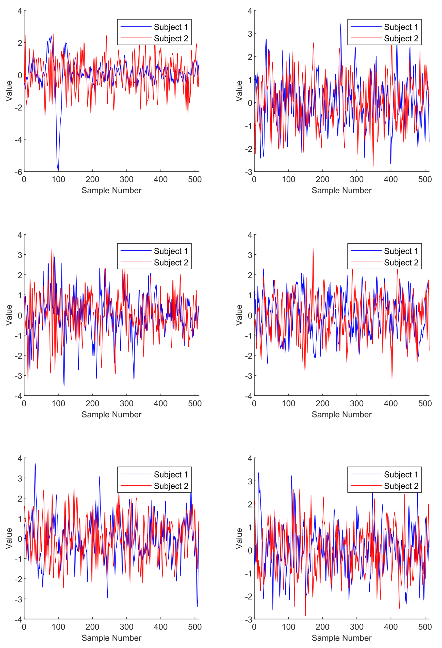
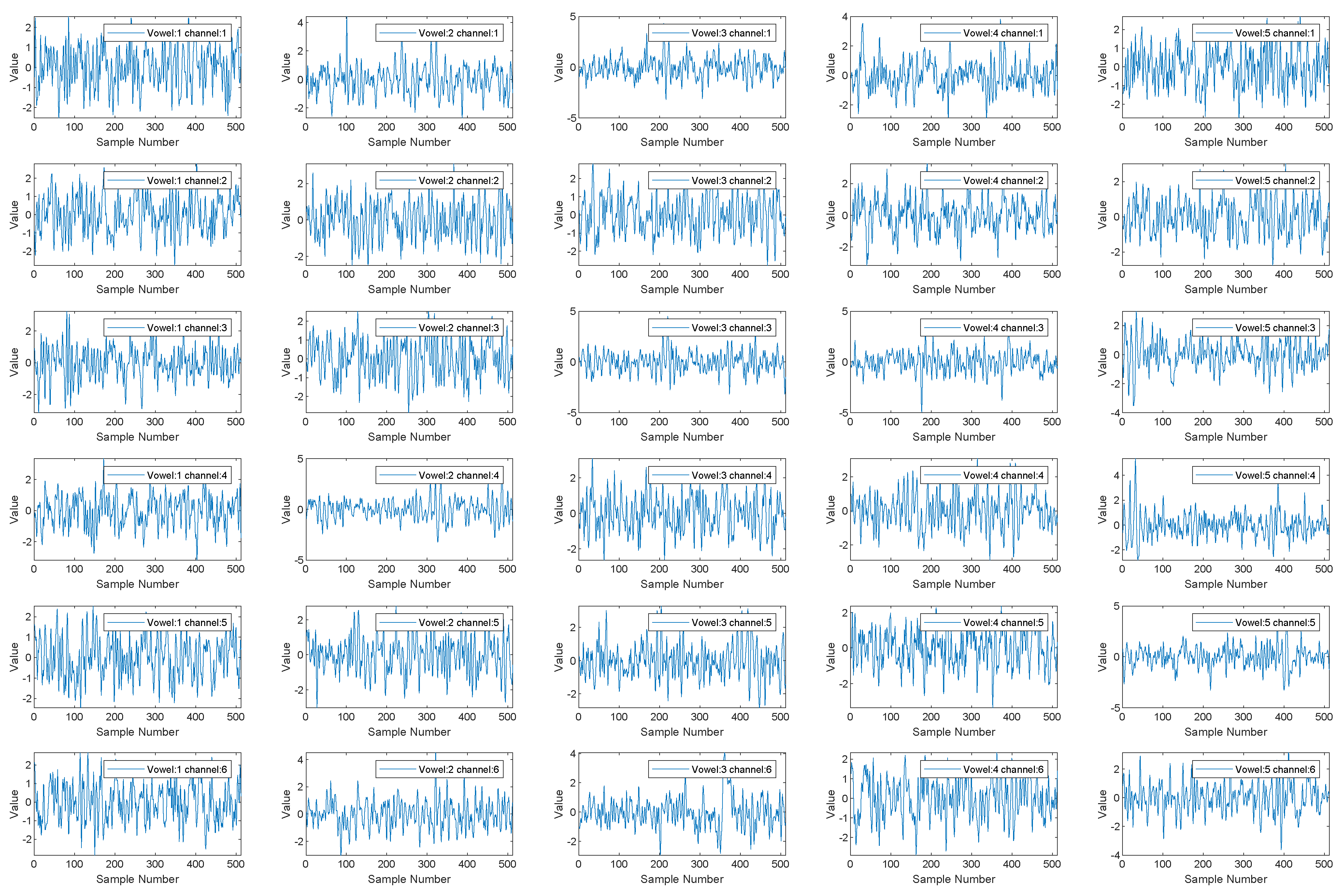
Appendix C. Dataset Samples


References
- Alderson-Day, B.; Fernyhough, C. Inner speech: Development, cognitive functions, phenomenology, and neurobiology. Psychol. Bull. 2015, 141, 931. [Google Scholar] [CrossRef] [PubMed]
- Whitford, T.J.; Jack, B.N.; Pearson, D.; Griffiths, O.; Luque, D.; Harris, A.W.; Spencer, K.M.; Le Pelley, M.E. Neurophysiological evidence of efference copies to inner speech. Elife 2017, 6, e28197. [Google Scholar] [CrossRef] [PubMed]
- Smallwood, J.; Schooler, J.W. The science of mind wandering: Empirically navigating the stream of consciousness. Annu. Rev. Psychol. 2015, 66, 487–518. [Google Scholar] [CrossRef] [PubMed]
- Filik, R.; Barber, E. Inner speech during silent reading reflects the reader’s regional accent. PLoS ONE 2011, 6, e25782. [Google Scholar] [CrossRef] [PubMed][Green Version]
- Langland-Hassan, P.; Vicente, A. Inner Speech: New Voices; Oxford University Press: New York, NY, USA, 2018. [Google Scholar]
- Zhao, S.; Rudzicz, F. Classifying phonological categories in imagined and articulated speech. In Proceedings of the 2015 IEEE International Conference on Acoustics, Speech and Signal Processing (ICASSP), South Brisbane, QLD, Australia, 19–24 April 2015; pp. 992–996. [Google Scholar]
- Cooney, C.; Folli, R.; Coyle, D. Optimizing layers improves CNN generalization and transfer learning for imagined speech decoding from EEG. In Proceedings of the 2019 IEEE International Conference on Systems, Man and Cybernetics (SMC), Bari, Italy, 6–9 October 2019; pp. 1311–1316. [Google Scholar]
- Coretto, G.A.P.; Gareis, I.E.; Rufiner, H.L. Open access database of EEG signals recorded during imagined speech. In Proceedings of the 12th International Symposium on Medical Information Processing and Analysis, Tandil, Argentina, 5–7 December 2017; Volume 10160, p. 1016002. [Google Scholar]
- Herff, C.; Heger, D.; De Pesters, A.; Telaar, D.; Brunner, P.; Schalk, G.; Schultz, T. Brain-to-text: Decoding spoken phrases from phone representations in the brain. Front. Neurosci. 2015, 9, 217. [Google Scholar] [CrossRef] [PubMed]
- Martin, S.; Iturrate, I.; Millán, J.d.R.; Knight, R.T.; Pasley, B.N. Decoding inner speech using electrocorticography: Progress and challenges toward a speech prosthesis. Front. Neurosci. 2018, 12, 422. [Google Scholar] [CrossRef] [PubMed]
- Dash, D.; Wisler, A.; Ferrari, P.; Davenport, E.M.; Maldjian, J.; Wang, J. MEG sensor selection for neural speech decoding. IEEE Access 2020, 8, 182320–182337. [Google Scholar] [CrossRef] [PubMed]
- Dash, D.; Ferrari, P.; Wang, J. Decoding imagined and spoken phrases from non-invasive neural (MEG) signals. Front. Neurosci. 2020, 14, 290. [Google Scholar] [CrossRef] [PubMed]
- Yoo, S.S.; Fairneny, T.; Chen, N.K.; Choo, S.E.; Panych, L.P.; Park, H.; Lee, S.Y.; Jolesz, F.A. Brain–computer interface using fMRI: Spatial navigation by thoughts. Neuroreport 2004, 15, 1591–1595. [Google Scholar] [CrossRef] [PubMed]
- Kamavuako, E.N.; Sheikh, U.A.; Gilani, S.O.; Jamil, M.; Niazi, I.K. Classification of overt and covert speech for near-infrared spectroscopy-based brain computer interface. Sensors 2018, 18, 2989. [Google Scholar] [CrossRef] [PubMed]
- Rezazadeh Sereshkeh, A.; Yousefi, R.; Wong, A.T.; Rudzicz, F.; Chau, T. Development of a ternary hybrid fNIRS-EEG brain–computer interface based on imagined speech. Brain-Comput. Interfaces 2019, 6, 128–140. [Google Scholar] [CrossRef]
- Panachakel, J.T.; Ramakrishnan, A.G. Decoding covert speech from EEG-A comprehensive review. Front. Neurosci. 2021, 15, 642251. [Google Scholar] [CrossRef] [PubMed]
- Schirrmeister, R.T.; Springenberg, J.T.; Fiederer, L.D.J.; Glasstetter, M.; Eggensperger, K.; Tangermann, M.; Hutter, F.; Burgard, W.; Ball, T. Deep learning with convolutional neural networks for EEG decoding and visualization. Hum. Brain Mapp. 2017, 38, 5391–5420. [Google Scholar] [CrossRef] [PubMed]
- Angrick, M.; Ottenhoff, M.C.; Diener, L.; Ivucic, D.; Ivucic, G.; Goulis, S.; Saal, J.; Colon, A.J.; Wagner, L.; Krusienski, D.J.; et al. Real-time synthesis of imagined speech processes from minimally invasive recordings of neural activity. Commun. Biol. 2021, 4, 1055. [Google Scholar] [CrossRef] [PubMed]
- Dash, D.; Ferrari, P.; Berstis, K.; Wang, J. Imagined, Intended, and Spoken Speech Envelope Synthesis from Neuromagnetic Signals. In Proceedings of the International Conference on Speech and Computer, St. Petersburg, Russia, 27–30 September 2021; pp. 134–145. [Google Scholar]
- Lawhern, V.J.; Solon, A.J.; Waytowich, N.R.; Gordon, S.M.; Hung, C.P.; Lance, B.J. EEGNet: A compact convolutional neural network for EEG-based brain–computer interfaces. J. Neural Eng. 2018, 15, 056013. [Google Scholar] [CrossRef] [PubMed]
- Nguyen, C.H.; Karavas, G.K.; Artemiadis, P. Inferring imagined speech using EEG signals: A new approach using Riemannian manifold features. J. Neural Eng. 2017, 15, 016002. [Google Scholar] [CrossRef] [PubMed]
- van den Berg, B.; van Donkelaar, S.; Alimardani, M. Inner Speech Classification using EEG Signals: A Deep Learning Approach. In Proceedings of the 2021 IEEE 2nd International Conference on Human-Machine Systems (ICHMS), Magdeburg, Germany, 8–10 September 2021; pp. 1–4. [Google Scholar]
- Nieto, N.; Peterson, V.; Rufiner, H.L.; Kamienkowski, J.E.; Spies, R. Thinking out loud, an open-access EEG-based BCI dataset for inner speech recognition. Sci. Data 2022, 9, 52. [Google Scholar] [CrossRef] [PubMed]
- Cooney, C.; Korik, A.; Folli, R.; Coyle, D. Evaluation of hyperparameter optimization in machine and deep learning methods for decoding imagined speech EEG. Sensors 2020, 20, 4629. [Google Scholar] [CrossRef] [PubMed]
- Ablin, P.; Cardoso, J.F.; Gramfort, A. Faster independent component analysis by preconditioning with Hessian approximations. IEEE Trans. Signal Process. 2018, 66, 4040–4049. [Google Scholar] [CrossRef]
- Cheng, J.; Zou, Q.; Zhao, Y. ECG signal classification based on deep CNN and BiLSTM. BMC Med. Inform. Decis. Mak. 2021, 21, 365. [Google Scholar] [CrossRef] [PubMed]
- Goodfellow, I.; Bengio, Y.; Courville, A. Deep Learning; MIT Press: Cambridge, MA, USA, 2016. [Google Scholar]


| Study | Technology | Number of Subjects | Number of Classes | Classifier | Results | Subject- Independent |
|---|---|---|---|---|---|---|
| 2015—[6] | EEG, facial | 6 | 2 phonemes | DBN | 90% | yes |
| 2017—[8] | EEG | 15 | 5 vowels | RF | 22.32% | no |
| 2017—[8] | EEG | 15 | 6 words | RF | 18.58% | no |
| 2017—[21] | EEG | 6 | 3 words | MRVM | no | |
| 2017—[21] | EEG | 6 | 2 words | MRVM | no | |
| 2018—[10] | ECoG | 5 | 2 (6) words | SVM | 58% | no |
| 2019—[7] | EEG | 15 | 5 vowels | CNN | 35.68 (with TL), 32.75% | yes |
| 2020—[24] | EEG | 15 | 6 words | CNN | 24.90% | no |
| 2020—[24] | EEG | 15 | 6 words | CNN | 24.46% | yes |
| 2019—[15] | fNIRS, EEG | 11 | 2 words | RLDA | 70.45% ± 19.19% | no |
| 2020—[12] | MEG | 8 | 5 phrases | CNN | 93% | no |
| 2021—[22] | EEG | 8 | 4 words | CNN | 29.7% | no |
| Study | Classifier | Vowels | Words |
|---|---|---|---|
| 2017—[8] | RF | 22.32% ± 1.81% | 18.58% ± 1.47% |
| 2019, 2020—[7,24] | CNN | 32.75% ± 3.23% | 24.90% ± 0.93% |
| iSpeech-GRU | GRU | 19.28% ± 2.15% | 17.28% ± 1.45% |
| iSpeech-CNN (proposed) | CNN | 35.20% ± 3.99% | 29.21% ± 3.12% |
| Vowel (iSpeech-CNN) | |||
| Precision | Weighted F-Score | F-Score | |
| No Downsampling | 34.85 | 41.12 | 28.45 |
| Downsampling | 34.62 | 38.99 | 30.02 |
| Cooney et al. [7] (Downsampling) | 33.00 | - | 33.17 |
| Words (iSpeech-CNN) | |||
| Precision | Weighted F-Score | F-Score | |
| No Downsampling | 29.04 | 36.18 | 21.84 |
| Downsampling | 26.84 | 31.94 | 21.50 |
Publisher’s Note: MDPI stays neutral with regard to jurisdictional claims in published maps and institutional affiliations. |
© 2022 by the authors. Licensee MDPI, Basel, Switzerland. This article is an open access article distributed under the terms and conditions of the Creative Commons Attribution (CC BY) license (https://creativecommons.org/licenses/by/4.0/).
Share and Cite
Simistira Liwicki, F.; Gupta, V.; Saini, R.; De, K.; Liwicki, M. Rethinking the Methods and Algorithms for Inner Speech Decoding and Making Them Reproducible. NeuroSci 2022, 3, 226-244. https://doi.org/10.3390/neurosci3020017
Simistira Liwicki F, Gupta V, Saini R, De K, Liwicki M. Rethinking the Methods and Algorithms for Inner Speech Decoding and Making Them Reproducible. NeuroSci. 2022; 3(2):226-244. https://doi.org/10.3390/neurosci3020017
Chicago/Turabian StyleSimistira Liwicki, Foteini, Vibha Gupta, Rajkumar Saini, Kanjar De, and Marcus Liwicki. 2022. "Rethinking the Methods and Algorithms for Inner Speech Decoding and Making Them Reproducible" NeuroSci 3, no. 2: 226-244. https://doi.org/10.3390/neurosci3020017
APA StyleSimistira Liwicki, F., Gupta, V., Saini, R., De, K., & Liwicki, M. (2022). Rethinking the Methods and Algorithms for Inner Speech Decoding and Making Them Reproducible. NeuroSci, 3(2), 226-244. https://doi.org/10.3390/neurosci3020017