Article

Predicting Fluid Intelligence via Naturalistic Functional Connectivity Using Weighted Ensemble Model and Network Analysis

1
Department of Computer Science, Swansea University, Swansea SA1 8EN, UK
2
Montreal Neurological Institute, McGill University, Montreal, QC H3A 2B4, Canada
3
Institute of Education, Sichuan Normal University, Chengdu 610066, China
*
Author to whom correspondence should be addressed.
Equally contribute to this study.
NeuroSci 2021, 2(4), 427-442; https://doi.org/10.3390/neurosci2040032
Submission received: 17 October 2021 / Revised: 24 November 2021 / Accepted: 3 December 2021 / Published: 17 December 2021
(This article belongs to the Special Issue Feature Papers in Neurosci 2021)

Abstract

:
Objectives: Functional connectivity triggered by naturalistic stimuli (e.g., movie clips), coupled with machine learning techniques provide great insight in exploring brain functions such as fluid intelligence. However, functional connectivity is multi-layered while traditional machine learning is based on individual model, which is not only limited in performance, but also fails to extract multi-dimensional and multi-layered information from the brain network. Methods: In this study, inspired by multi-layer brain network structure, we propose a new method, namely weighted ensemble model and network analysis, which combines machine learning and graph theory for improved fluid intelligence prediction. Firstly, functional connectivity analysis and graphical theory were jointly employed. The functional connectivity and graphical indices computed using the preprocessed fMRI data were then all fed into an auto-encoder parallelly for automatic feature extraction to predict the fluid intelligence. In order to improve the performance, tree regression and ridge regression models were stacked and fused automatically with weighted values. Finally, layers of auto-encoder were visualized to better illustrate the connectome patterns, followed by the evaluation of the performance to justify the mechanism of brain functions. Results: Our proposed method achieved the best performance with a 3.85 mean absolute deviation, 0.66 correlation coefficient and 0.42 R-squared coefficient; this model outperformed other state-of-the-art methods. It is also worth noting that the optimization of the biological pattern extraction was automated though the auto-encoder algorithm. Conclusion: The proposed method outperforms the state-of-the-art reports, also is able to effectively capture the biological patterns of functional connectivity during a naturalistic movie state for potential clinical explorations.

1. Introduction

The human brain can be viewed as a complex network with an enormous amount of locally segregated structural regions; although each region is dedicated to different functionalities, together they maintain globally functional communications among different cognitive resources. One of the most important non-invasive approaches to measure brain functional connectivity (FC) is the functional magnetic resonance imaging (fMRI), which reflects the changes in the blood oxygen level-dependent (BOLD) signal [1]. As one of the major advancements in recent fMRI data analyses, functional connectivity is used to measure the temporal dependency of neuronal activation patterns in different brain regions and the communications between these regions [2]. Traditional FC analysis was based on specific experimental paradigms or resting state; recent studies have shown that naturalistic stimuli, which forms ecologically valid paradigms and approximates real life, could improve compliance of the participants [3] and hence increase test-retest reliability [4]. Indeed, functional connectivity with high ecological validity assessed through naturalistic stimulus has been found more reliable than that assessed in the resting state [5]. Additionally, while exposed to this natural stimulus, the processing of sensory information would depend on the topological structure, especially the hierarchical and modular connections [6].
Many neuroimaging studies have shown that the relationship between biological function and cognitive function can be established using certain statistical measurements (e.g., Pearson correlation). However, statistical methods (e.g., parametric methods) tend to over-fit the data and yield a quantitatively increased certainty of the statistical estimates, while failing to generalize to novel data [7]. Furthermore, it may be impaired by high-dimensional situations (e.g., FC) [7]. On the other hand, machine learning methods with well-established processing standards could extract biological patterns and leverage individual-level prediction simultaneously from the neuroimaging data [8]. By further integrating FC analysis into the machine learning framework, a data-driven approach named connectome-based predictive modeling (CPM) could even predict individual differences in traits and behaviours [9]. Coupled with the alerting score method, Rosenberg et al. found that CPM could predict sustained attention ability using resting-state fMRI data; this finding may be applied to describe the new insight regarding the relationship between FC and cognitive ability [10]. In predicting fluid intelligence, Abigail et.al. found that a specific-task-based predictive model outperformed the resting-state-based model; this revealed that identifying the brain patterns in a given group could provide a unique brain-fluid intelligence relationship [11].
Using machine learning techniques, the physiologically important representations buried within fMRI data could also be excavated and captured [12]. For example, using deep learning and fMRI, Plis et al. found that deep nets could sift and keep the latent relation and biological patterns from neuroimaging data [13]. These studies indicate that deep neural nets not only could be used to infer the presence of brain-behavior (e.g., FC and human behavior) relationships and bring new representation to explain the neural mechanisms, but also can be used as the fingerprint to translate neuroimaging findings into practical utility [14]. However, traditional machine learning models based on a single model were limited in model generalization and model performance [9]. Previous studies have demonstrated that ensemble learning, proposed by Breiman et al. [15], has been integrated with bootstrap sampling and multiple classifiers to improve generalization. In addition, the overfitting issue would also be eliminated by using ensemble learning [16]. Inspired by the fact that the brain networks are hierarchical with information processed in different layers [6], combining hierarchical structure and ensemble learning could be an effective way to improve the performance of models and extract biological information from data.
In this study, we propose a new machine learning hierarchical structure to predict the fluid intelligence (reflects basic cognitive ability), using the biological patterns extracted by examining the naturalistic functional connectivity. A new regression method based on machine learning and graph theory, namely weighted ensemble model and network analysis (WENA), has been developed for this prediction problem. Compared with the traditional CPM, we used a self-supervised learning method named auto-encoder (AE) to extract non-linear and deep information from the functional connectivity measurements and the graphical theory indices based on fMRI data. To further boost the prediction performance, we also proposed a novel approach, namely weighted stacking (WS), which comprised of a multi-stacking layer structure for WENA to improve the effectiveness of model fusion. The comparative analysis showed that the proposed method outperforms the state-of-the-art methods reported. The results also revealed the existing coherence between biological fluid intelligence and neuroimaging reflection using the proposed data-driven approach.

2. Materials and Methods

2.1. Data Acquisition

The data of 464 participants, aged from 18 to 88 years old, were downloaded from the population-based sample of the Cambridge Centre for Ageing and Neuroscience (Cam-CAN, http://www.cam-can.com, accessed on 10 December 2021). The subjects without behavioral/demographical data and/or neuroimaging data (fMRI or MRI) were excluded from this study; hence, in total, 461 control participants without mental illnesses and neurological disorders were included in this work. The fluid intelligence score (FIS) and demographical information about the participants are shown in Table 1.
The fMRI data were recorded while subjects were watching a clip of the movie by Alfred Hitchcock named “Bang! You’re Dead”. According to a previous neural synchronization study, the full 25-min episode was condensed to 8 min [17]. Participants were instructed to watch, listen, and pay attention to the movie.
The data were collected using a 3T Siemens TIM Trio System with a 32-channel head coil at the MRC Cognition Brain and Science Unit, Cambridge, UK. For each participant, a 3D-structural MRI was obtained using a T1-weighted sequence (generalized auto-calibrating partially parallel acquisition; repetition time = 2250 ms; echo time = 2.99 ms; inversion time = 900 ms; flip angle α = 9°; matrix size 256 mm × 240 mm × 19 mm; field of view = 256 mm × 240 mm × 192 mm; resolution = 1 mm isotropic; accelerated factor = 2) during the movie-watching period.

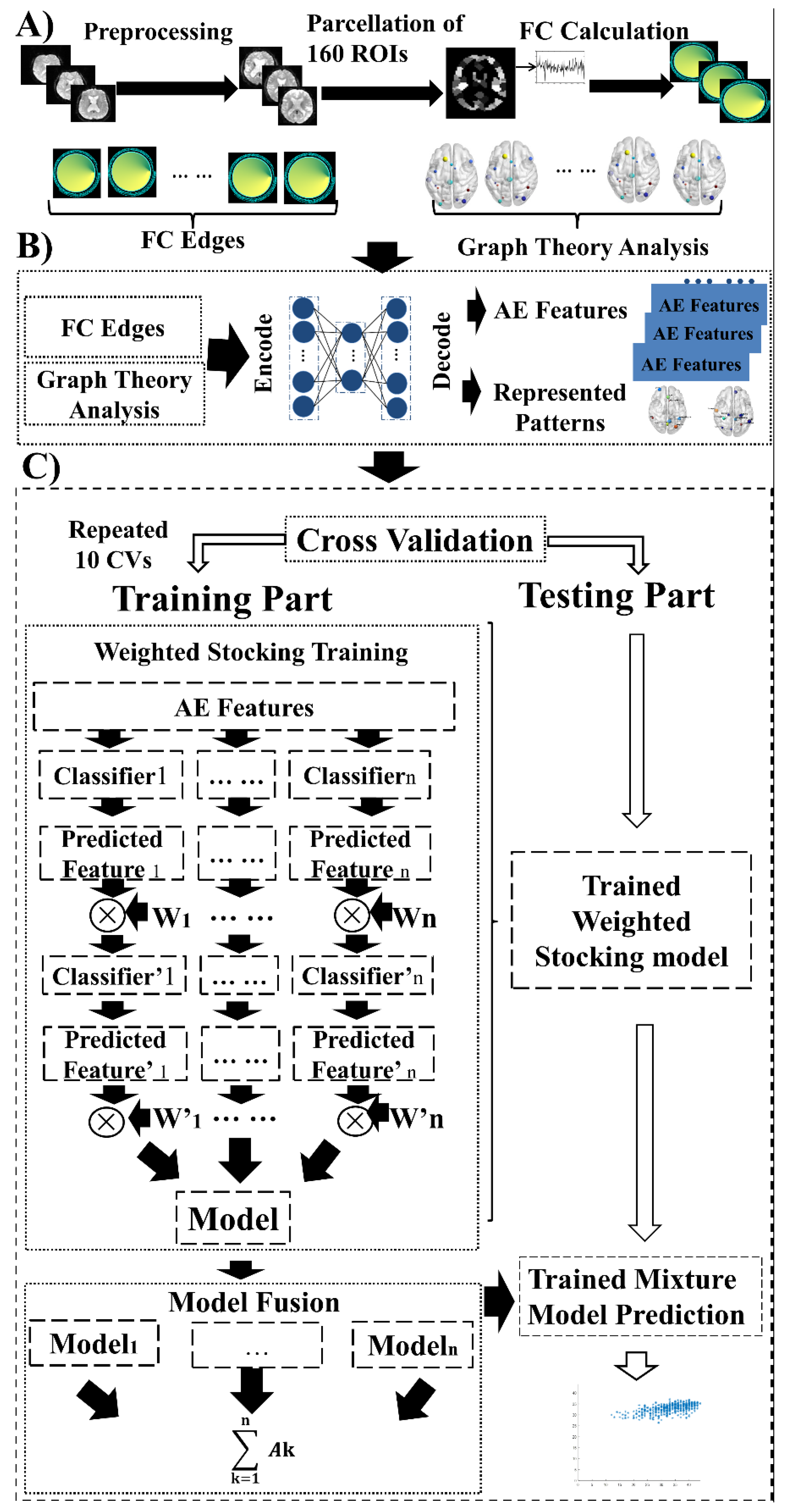
2.2. Experimental Pipeline

To predict the brain fluid intelligence, the proposed WENA method is integrated with a series of models via hierarchically functional networks. Figure 1 illustrates the overall structure of the system. To start with, the raw fMRI data was preprocessed and the FCs (12,720 FCs for each subject) from 160 regions of interest (ROIs) computed; the graphical theory indices (including degree centrality, the ROI’s strength, local efficiency and betweenness centrality) were also obtained in parallel within this step. The indices were entered into the AE module and encoded as AE features; decoded AE patterns were then obtained. Finally, all features were fed into WS structure to obtain the FIS for each subject.

2.3. Data Preprocessing

Data preprocessing was carried out using the Data Processing Assistant for Statistical Parametric Mapping (SPM8, http://www.fil.ion.ucl.ac.uk/spm, accessed on 10 December 2021) and a few necessary hand-crafted MATLAB scripts (MATLAB 2018a). Initially, the first 5 volumes were discarded to reduce the impact from the instability of the magnetic field. The preprocessing procedure consisted of naturalistic fMRI-included slice-timing correction, realignment, spatial normalization (3 × 3 × 3 mm3) and smoothing [6 mm full width at half maximum (FWHM)]. First, slice-timing corrections were used for different signal acquisitions between each slice and motion effect (6 head motion parameters). The possible nuisance signals, which include linear trends, global signals, and individual mean WM and CSF signals, were removed via multiple linear regression analysis and temporal band-pass filtering (pass band 0.01–0.08 Hz). The calculation of head motion was done according to the following formula:
Head _ Motion = 1 M - 1 | d x i 1 | 2 + | d y i 1 | 2 + | d z i 1 | 2 + | d x i 2 | 2 + | d y i 2 | 2 + | d z i 2 | 2
where M represents the number of time points of each subject; d x i 1 / d x i 2 , d y i 1 / d y i 2 and d z i 1 / d z i 2 are translations/rotations at each time point in the x, y and z planes. d x i 1 represents the difference between x i 1 and   x i 1 1 . Furthermore, the subjects with translational motion > 2.5 mm, rotation > 2.5°, and mean absolute head displacement (mFD) > 0.5 mm were excluded in this study. Next, the fMRI data were spatially normalized to the Montreal Neurological Institute (MNI) space by using Dosenbach [18]. Finally, the fMRI data were smoothed with a Gaussian kernel of 6 mm full width at half maximum (FWHM) to decrease spatial noise.

2.4. Functional Connectivity and Network Property

For each participant, the whole-brain functional connectivities between all 160 brain regions were constructed pairwise from the preprocessed fMRI data, according to Dosen Bash [18]. The FCs for each ROI pair computed using the Pearson’s correlation (PC), mutual information (MI) [19] and distance correlation (DistCorr) [20] were calculated respectively, then further averaged over time toward the BOLD signals per subject. Once the whole-brain network was available, numerous measures could be expressed in terms of a graph. A threshold (the highest 20% of the weights) was set to sparse the constructed network. Graph theory analysis was performed on the sparse network for each subject with different FC calculation strategies. The graph theory indices included the degree centrality (DC), the ROI’s strength (RS), local efficiency (LE) and betweenness centrality (BC). Specifically, DC is the number of existing connections among target nodes. RS is the average strength of existing connections that relates to the same target node. The LE of a node is the average of the inverse of the minimum path length between the target node and other nodes. The BC of a node is the number of shortest paths between two nodes [21]. Finally, the features based on FC and graph theory indices were used for further feature representation via AE and regression.

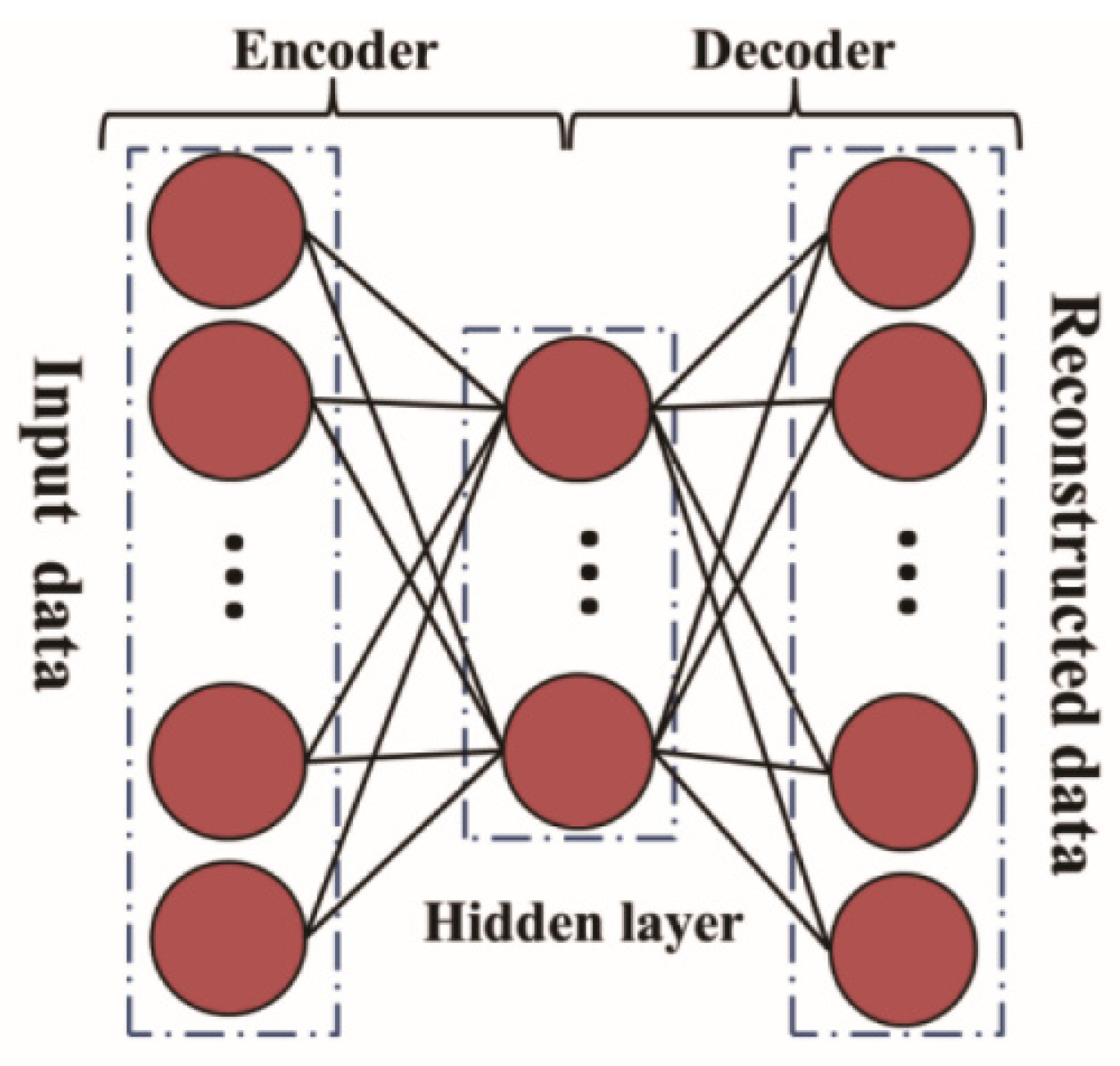
2.5. Feature Encoder and Network Pattern Construction

Each subject’s Nnode × Nnode connectivity matrices, which were concatenated to give an Nsubject × Nedge matrix (fully weighted), and graph theory indices, which were an Nsubject × Ngraph indices matrix, were then entered into AE (Figure 1A). The number of epochs was 500 and the hidden nodes was set to 50 [22]. The AE, illustrated in Figure 2, is a special type of neural network which is capable of conduct feature engineering. All models were initially trained using different AE features; these features were extracted from network patterns and graphical indices. To prevent overfitting and accuracy bias due to the reuse of the same data, the extracted features were split into training and test sets for 10-fold cross-validation. The vectors x R were encoded into hidden representation h R by the activation function   f :
h = f ( Wx + b )
The hidden representation h was decoded to reconstruct the data h R by the activation function:
r = g ( W h + b )
where W and W’ are the weight matrices, b and b’ represent the bias vectors, and the classic sigmoid ( x ) = 1/(1 + e x ) has been adopted as the activation function for f and g.
Effectively a nonlinear principal components analysis (PCA) [23], the AE can be trained in a fully unsupervised manner. The AE seeks the optimal parameters W, W’, b and b’ via the gradient descent algorithm to minimize the reconstruction error   L ( x , r ) = x r 2 . In order to prevent overfitting, a weighted constraint parameter was used to regularize   L ( x , r ) , as shown in Equation (4), where ε is the regularization parameter.
L ( x , r ) = L ( x , r ) + ε W 2 2
The whole-brain FC was then entered into the AE to extract and preserve the main information of the network, according to the loss function minimum criterion [24].

2.6. Weighted Ensemble Models and Network Analysis Framework

All models were initially trained using different AE features; these features were extracted from network patterns and graphical indices. Predictive models were implemented and merged using a multi-stacking layer approach, namely weighted stacking (WS). On its first layer, basic regression models were used to predict FIS from neuroimaging data. Weighted operators were then obtained to measure the performance of each model. The formula of the weight operator W is shown in (5).
W i = Correlation   Coefficient i Mean   Absolute   Error i i = 1 n Correlation   Coefficient i Mean   Absolute   Error i
where n is the number of features, correlation coefficient refers to the correlation between the real label and predicted label of each first-level training model, and mean absolute error measures the absolute error between the real label and predicted label of each first-layer training model.
On the second layer, predictions from the first-level models were multiplied by the W coefficient and then stacked with other regression models. Finally, the fusion factors were set to fuse the weighted stacking models, and fusion operator W’ was defined in (6).
W j = Correlation   Coefficient j Mean   Absolute   Error j j = 1 m Correlation   Coefficient j Mean   Absolute   Error j
where m is the number of regression models, correlation coefficient indicates the correlation coefficient between the real label and predicted label of each second-level training model, and mean absolute error is the mean absolute error between the real label and predicted label of each second-layer training model.
In this study, the basic regression models employed for WENA were the ensemble tree regression (ETR) and ridge regression (RR) models. A support vector regression (SVR) model with Gaussian kernel and an extreme learning machine regression (ELMR) model were also used to compare with the performance of WENA and test the robustness of the proposed framework.

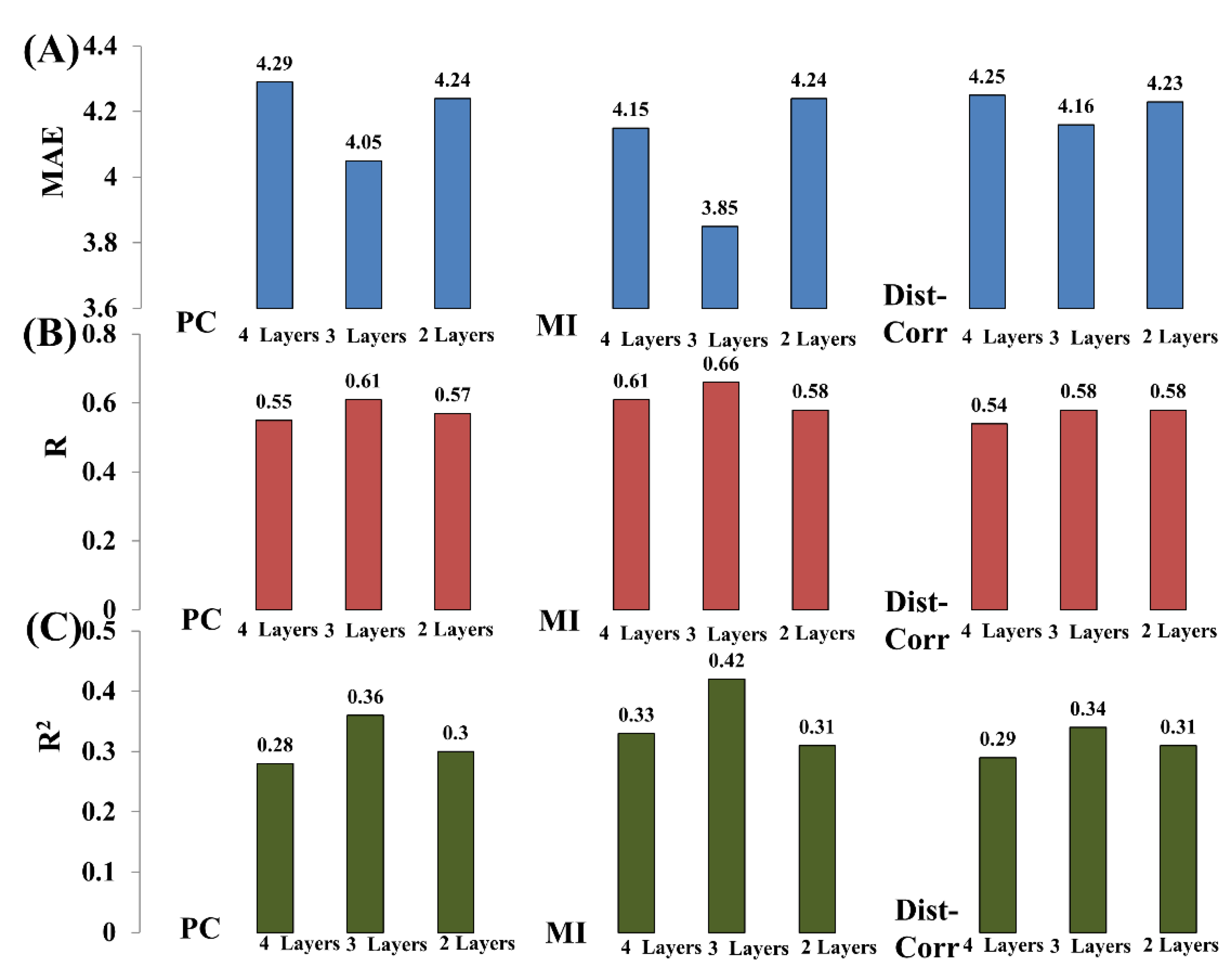
2.7. Parameter Test of Proposed WENA

To further explore the impact of the model parameters, the stacking layers from 2 layers to 4 layers with different FC construction methods and model fusion strategies were used to train the WENA model. Additionally, in order to reduce the effect of other parameters on performance, different regression models were trained via the same set of AE features.

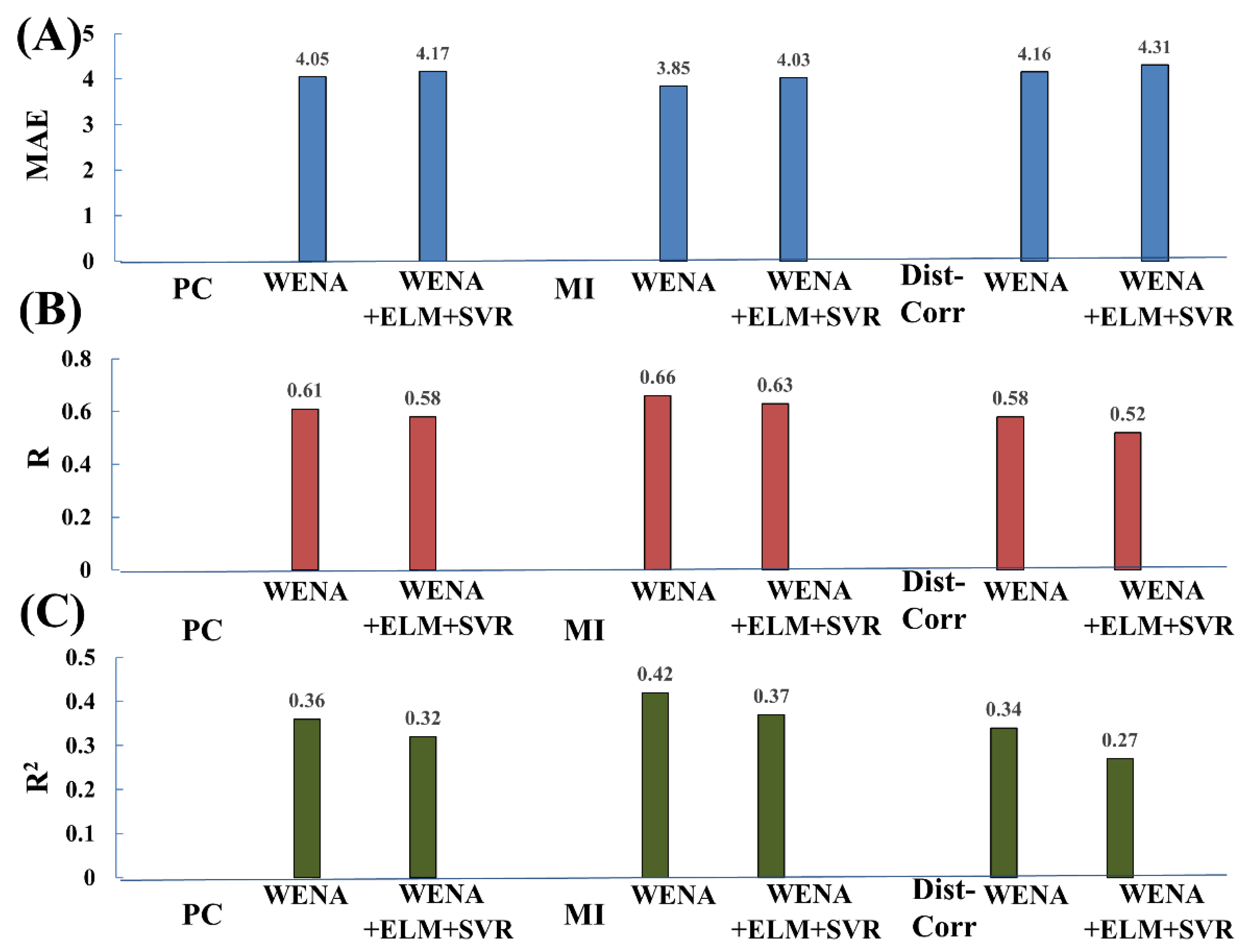
2.8. Methods Comparison

In this study, we compared the performance of WENA against a range of conventional stacking-structure regressions, including the ETR, RR, SVR and ELMR models. Each FC pattern and network property was fed for the principal component analysis (PCA) and independent component analysis (ICA), respectively. The dimension reduction number of PCA and ICA is in consistent with the AE. Extracted features were used to train the WENA framework; the results were also compared with using AE methods for feature extraction. All methods were tested in features based on three FC construction methods.

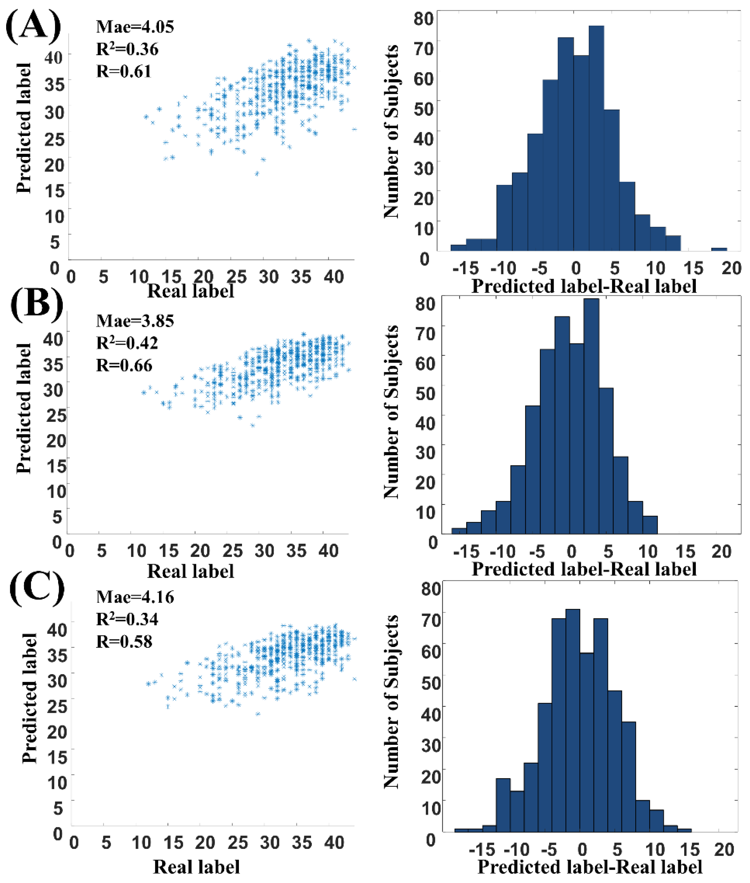
3. Evaluation Metrics

The mean absolute deviation (MAE), Pearson correlation coefficient (R value) and R-squared coefficient (R2 value) between the real values and predicted values were used to evaluate the performance of the proposed method.

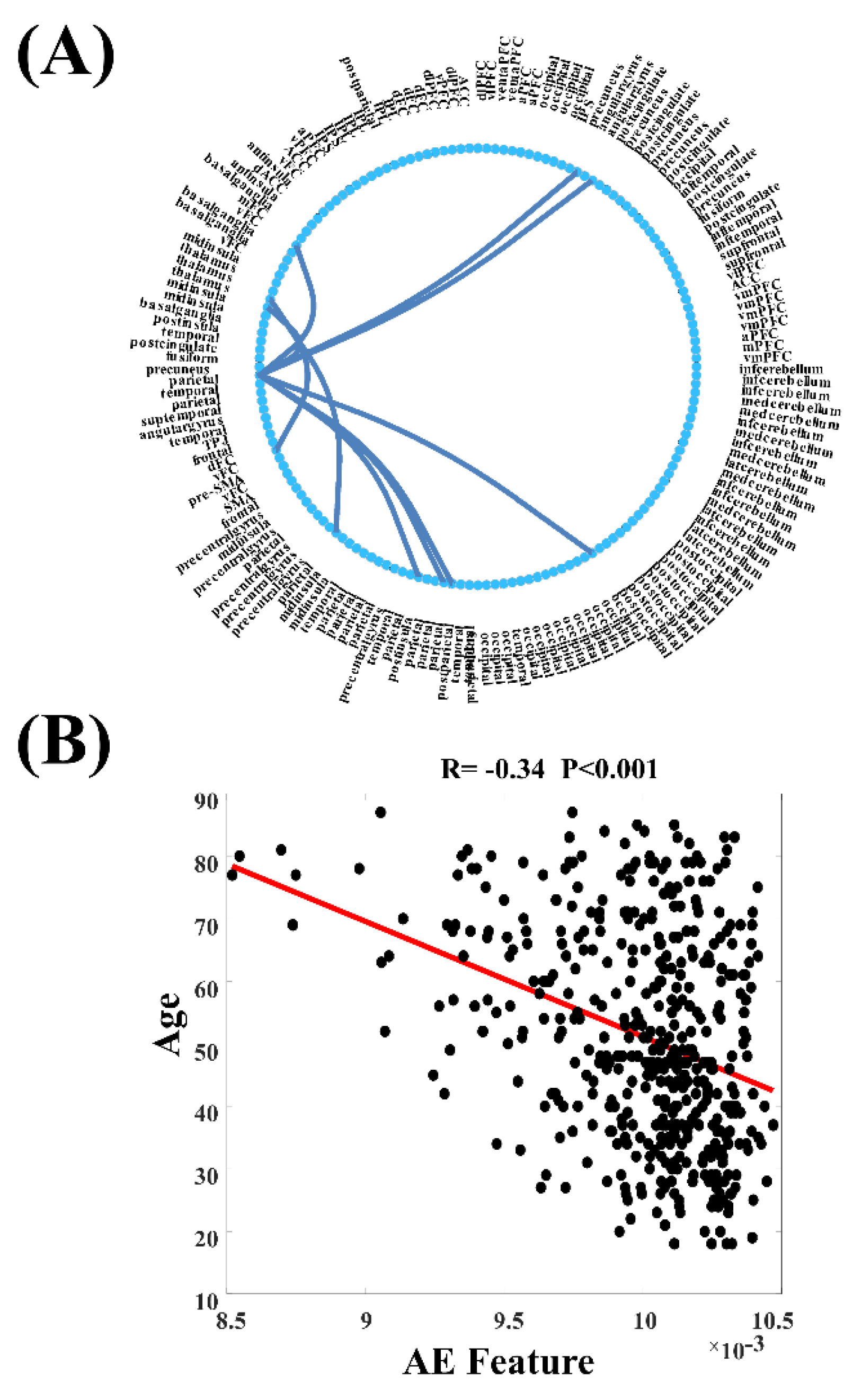
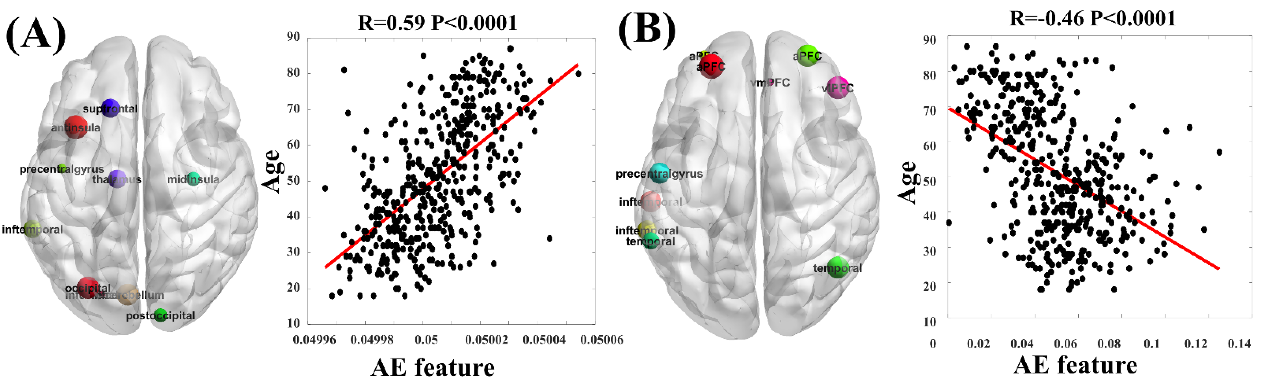
Biological Pattern Visualization

Each AE feature was evaluated by using the RelifF method [25], and the feature with the largest RelifF value was considered to be the biomarker with biological significance. Pearson correlation was used to evaluate the relationship between age and AE features to extract age-related and biological patterns. The biological patterns corresponding to the chosen AE features were extracted via the weight value of the AE and visualized [26].

4. Experiment Results

We compared the performance of WENA method with different weighted stacking models and FC construction methods. Table 2 illustrated that the proposed WENA achieved the best performance for fluid intelligence prediction across three functional connectivity construction methods. The performance of MI-based features obtained the highest performance with an MAE of 3.85, an R value of 0.66 and an R2 value of 0.42. The best FIS prediction of each network construction was shown in Figure 3. Furthermore, conventional stacking structures and feature engineering methods were used to compare with the proposed WENA method based on AE features. Table 3 showed that the conventional stacking model based on SVR achieved the best performance (the MAE was 4.25, R value was 0.53, and R2 was 0.26), while the PC network construction method and basic SVR model achieved the best MAE, with a value of 4.20 (the R value was 0.53 and R2 was 0.28). Compared with conventional feature engineering methods with the MI network construction method, WENA achieved the following performance: MAE of 4.12, an R value of 0.58 and an R2 value of 0.33 for PCA methods; and MAE of 4.77, an R value of 0.32 and an R2 value of 0.10 for ICA methods.
Stacking layers and model fusion strategies were used to test the robustness of the proposed WENA. Figure 4 showed that the number of stacking layers could affect the performance of WENA, and that the three-layer structure was optimized. Additionally, Table 3 showed that the proposed WENA method outperformed conventional stacking models which were without the WS structure and single basic regression models without a stacking structure. Furthermore, both Figure 4 and Table 3 revealed that the proposed WENA method was robust to different FC construction methods. Figure 5 showed that WENA including the ETR and RR models outperformed WENA integrated with other regression models, including SVR and ELM models.
It has been noticed that there was a significant correlation between age and FIS (R = 0.65, p < 0.001). There were also substantial differences between the network AE feature and age in the FC pattern (R = −0.34, p < 0.001), BC pattern (R = 0.59, p < 0.001) and LE pattern (R = 0.46, p < 0.001), while there was no significant relationship found between other graph theory indices (DC and RS) and age. The most discriminative age-related FC with network-property patterns was visualized via AE, as well as the important ROIs extracted by WENA (shown in Figure 4 and Figure 6, Table 4, Table 5 and Table 6). These results revealed that the most biological patterns extracted by WENA were the sensorimotor network, cingulo-opercular network, occipital network and cerebellum network.

5. Discussion

In this study, we have developed a new regression method based on machine learning and graph theory namely WENA, to extract biological patterns from functional connectivity and predict fluid intelligence effectively. The results indicate that (a) the proposed method outperforms the state-of-the-art reports; (b) our proposed framework is robust toward different network construction methods and variables; (c) the patterns extracted using this method have been found with interesting biological interpretations. These patterns were significantly related to age, which are found may stem from the sensorimotor network, cingulo-opercular network, occipital network and cerebellum network.
The proposed WENA architecture also outperforms other traditional methods in terms of FIS prediction (shown in Table 2, Table 3 and Table 4). In particular, ensemble learning models (including bagging, stacking and boosting), which consisted of several single machine learning models [30], outperformed the single machine learning model. The single machine learning algorithm was limited in model generalization and model performance [9], while the performance of ensemble learning could be improved via using bootstrap replicates, and bagging could be further improved via stacking [31]. Unlike deep learning, which risks overfitting and lacking model generalization [32], ensemble learning could integrate with bootstrap samples and multiple classifiers, which could lead to the enhancement of model generalization and reduction of model overfitting [15,33].
The proposed WENA based on WS methods and model fusion also outperformed traditional stacking methods (see Table 3). The proposed method was based on a self-supervised learning mechanism (AE); it could extract non-linear features and principal modes from FC data across a population [34]. It also has been found that the performance of WENA based on WS outperformed that of WENA based on principal component analysis (PCA) and independent component analysis (ICA) (see Table 4). As traditional approaches in neuroscience, PCA and ICA were both for linear features, the performances based on PCA features and ICA features were influenced by their unsupervised dimension reduction nature [35]. By contrast, the AE could represent high-layer features and abstract low-level features (e.g., cerebrospinal fluid, cortical thickness and gray matter tissue volume) from neuroimaging data, also create general latent feature representation and improve the performance [12,36]. For example, via the AE and fMRI, Suk et al. extracted nonlinear hidden features from neuroimaging data and improved diagnostic accuracy [36].
However, it should be noted that the network construction methods were used and compared in this study (shown in Table 1), and our results showed that the performance of machine learning is impacted by FC construction methods (shown in Table 1 and Table S1). For example, while WENA was robust to network construction methods for improving the performance of FIS prediction, however, the number of stacking layers and the regression methods could affect the performance of WENA (seen in Figure 4 and Figure 7). In all, our results revealed that the proposed WENA model achieved the best regression accuracy on FC constructed via MI methods (MAE = 3.85, R = 0.66, R2 = 0.42). Furthermore, the proposed WENA was better than other conventional methods and the state-of-the-art (shown in Table 4).
The proposed WENA methods achieved improvements in the prediction of fluid intelligence from neuroimaging data, it was also able to decode the biological age-related patterns from the naturalistic fMRI data (shown in Table 3). Fluid intelligence, as a highly age-related cognitive trait, could offer objective evidence in understanding naturalistic neuroimaging data for the ageing problem. For example, fluid intelligence, the ability to think and solve problems under limited knowledge situations [37], tends to decline with ageing due to reductions in the executive function of the prefrontal cortex [38]. In our study, FIS was positively correlated to age, and extracted AE features were negatively related to age (p < 0.05). Furthermore, the functional networks extracted via the AE spatial filter were the sensorimotor network, cingulo-opercular network, occipital network and cerebellum network. To be specific, AE features which corresponded to the sensorimotor network and the cerebellum network were significantly positively correlated to age, which demonstrated compensatory existing age-related decline in motor function [39]. In line with our study, the existence of increased sensorimotor and cerebellum functional connectivity has been found in elders, supporting the previous report on the increased interactivities found across the networks with ageing [40]. Similarly, AE features which corresponded to the cingulo-opercular network and occipital network were significantly negatively associated with age, also in line with previous studies [41]. Previous studies have also shown that the sensorimotor network was associated with sensory processing and the occipital network was related to visual preprocessing [41]. Additionally, the cingulo-opercular network, also referred to as the salience network, decreased with age, which was the neural factor that affected visual processing speed [42]. These brain functions were closely related to movie-watching experience and ageing issues, as well as fluid intelligence. Therefore, these studies supported that our methods could decode biological patterns and revealed that network patterns, consisting of the sensorimotor, cingulo-opercular, occipital and cerebellum networks, contributed to the prediction of fluid intelligence as well as the ageing problem.
However, several limitations should be noted. Firstly, the WENA model was unable to clearly reflect the quantitative relationship between age, functional connectivity and fluid intelligence. Secondly, the robustness of the proposed methods should be further tested using samples from other resources. Finally, the overfitting problem in the training dataset should be carefully considered, though ensemble learning could reduce it to some degree.

6. Conclusions

In this study, we have proposed a new method, namely WENA, to predict fluid intelligence and mine deep network information through naturalistic fMRI data, which is based on ensemble learning, FC analysis and graph theory analysis. The results indicate that the proposed method outperformed mainstream state-of-the-art methods for the problem of interest. As a deep network, once the classifier choice and stack level have been optimized, the performance of WENA is found to be rather robust. Special ageing-related network patterns and their property patterns were also able to be extracted via WENA. It was found that the sensorimotor, cingulo-opercular and occipital-cerebellum regions are the most impactful regions for the prediction of fluid intelligence. Our future work will focus on addressing the existing limitations of the proposed method, hence better predicting human behavior and observing human brain states.

Supplementary Materials

The following are available online at https://www.mdpi.com/article/10.3390/neurosci2040032/s1, Table S1. The performance of conventional stacking models and single models. Table S2. The performance of different feature method based on MI features. Figure S1. The influence of stacking-level on performance, including MAE, R value and R2 value. Figure S2. The influence of regression models choice on performance of WENA with different network construction methods.

Author Contributions

X.L. was responsible for method proposal, data analysis and manuscript writing. S.Y. was responsible for revision of the manuscript. Z.L. was responsible for revision of the manuscript and funding acquisition of the project. All authors have read and agreed to the published version of the manuscript.

Funding

This study was funded by the China Scholarship Council and the National Social Science Foundation of China (BEA200115).

Institutional Review Board Statement

Not applicable.

Informed Consent Statement

Not applicable.

Data Availability Statement

The data presented in this study are available in the main text, figures, tables and supplementary material.

Conflicts of Interest

The authors declare no conflict of interest.

References

  1. Logothetis, N.K.; Wandell, B.A. Interpreting the BOLD signal. Annu. Rev. Physiol. 2004, 66, 735–769. [Google Scholar] [CrossRef] [PubMed]
  2. Van Den Heuvel, M.P.; Pol, H.E.H. Exploring the brain network: A review on resting-state fMRI functional connectivity. Eur. Neuropsychopharmacol. 2010, 20, 519–534. [Google Scholar] [CrossRef] [PubMed]
  3. Centeno, M.; Tierney, T.M.; Perani, S.; Shamshiri, E.A.; StPier, K.; Wilkinson, C.; Konn, D.; Banks, T.; Vulliemoz, S.; Lemieux, L. Optimising EEG-fMRI for localisation of focal epilepsy in children. PLoS ONE 2016, 11, e0149048. [Google Scholar]
  4. Sonkusare, S.; Breakspear, M.; Guo, C. Naturalistic Stimuli in Neuroscience: Critically Acclaimed. Trends Cogn. Sci. 2019, 23, 699–714. [Google Scholar] [CrossRef] [PubMed]
  5. Wang, J.; Ren, Y.; Hu, X.; Nguyen, V.T.; Guo, L.; Han, J.; Guo, C.C. Test–retest reliability of functional connectivity networks during naturalistic fMRI paradigms. Hum. Brain Mapp. 2017, 38, 2226–2241. [Google Scholar] [CrossRef] [Green Version]
  6. Lynn, C.W.; Papadopoulos, L.; Kahn, A.E.; Bassett, D.S. Human information processing in complex networks. Nat. Phys. 2020, 16, 965–973. [Google Scholar] [CrossRef]
  7. Bzdok, D.; Altman, N.; Krzywinski, M. Points of significance: Statistics versus machine learning. Nat. Methods 2018, 2018, 1–7. [Google Scholar]
  8. Bzdok, D.; Meyer-Lindenberg, A. Machine learning for precision psychiatry: Opportunities and challenges. Biol. Psychiatr. Cogn. Neurosci. 2018, 3, 223–230. [Google Scholar] [CrossRef] [Green Version]
  9. Shen, X.; Finn, E.S.; Scheinost, D.; Rosenberg, M.D.; Chun, M.M.; Papademetris, X.; Constable, R.T. Using connectome-based predictive modeling to predict individual behavior from brain connectivity. Nat. Protoc. 2017, 12, 506. [Google Scholar] [CrossRef] [Green Version]
  10. Rosenberg, M.D.; Hsu, W.-T.; Scheinost, D.; Todd Constable, R.; Chun, M.M. Connectome-based models predict separable components of attention in novel individuals. J. Cogn. Neurosci. 2018, 30, 160–173. [Google Scholar] [CrossRef]
  11. Greene, A.S.; Gao, S.; Scheinost, D.; Constable, R.T. Task-induced brain state manipulation improves prediction of individual traits. Nat. Commun. 2018, 9, 2807. [Google Scholar] [CrossRef] [PubMed] [Green Version]
  12. Huang, H.; Hu, X.; Zhao, Y.; Makkie, M.; Dong, Q.; Zhao, S.; Guo, L.; Liu, T. Modeling task fMRI data via deep convolutional autoencoder. IEEE Trans. Med. Imaging 2017, 37, 1551–1561. [Google Scholar] [CrossRef] [PubMed]
  13. Plis, S.M.; Hjelm, D.R.; Salakhutdinov, R.; Allen, E.A.; Bockholt, H.J.; Long, J.D.; Johnson, H.J.; Paulsen, J.S.; Turner, J.A.; Calhoun, V.D. Deep learning for neuroimaging: A validation study. Front. Neurosci. 2014, 8, 229. [Google Scholar] [CrossRef] [Green Version]
  14. Finn, E.S.; Shen, X.; Scheinost, D.; Rosenberg, M.D.; Huang, J.; Chun, M.M.; Papademetris, X.; Constable, R.T. Functional connectome fingerprinting: Identifying individuals using patterns of brain connectivity. Nat. Neurosci. 2015, 18, 1664. [Google Scholar] [CrossRef]
  15. Breiman, L.; Last, M.; Rice, J. Random Forests: Finding Quasars. In Statistical Challenges in Astronomy; Springer: New York, NY, USA, 2003. [Google Scholar]
  16. Kesler, S.R.; Rao, A.; Blayney, D.W.; Oakleygirvan, I.A.; Karuturi, M.; Palesh, O. Predicting Long-Term Cognitive Outcome Following Breast Cancer with Pre-Treatment Resting State fMRI and Random Forest Machine Learning. Front. Hum. Neurosci. 2017, 11, 555. [Google Scholar] [CrossRef] [Green Version]
  17. Taylor, J.R.; Williams, N.; Cusack, R.; Auer, T.; Shafto, M.A.; Dixon, M.; Tyler, L.K.; Henson, R.N. The Cambridge Centre for Ageing and Neuroscience (Cam-CAN) data repository: Structural and functional MRI, MEG, and cognitive data from a cross-sectional adult lifespan sample. Neuroimage 2017, 144, 262–269. [Google Scholar] [CrossRef]
  18. Dosenbach, N.U.; Nardos, B.; Cohen, A.L.; Fair, D.A.; Power, J.D.; Church, J.A.; Nelson, S.M.; Wig, G.S.; Vogel, A.C.; Lessov-Schlaggar, C.N.; et al. Prediction of individual brain maturity using fMRI. Science 2010, 329, 1358–1361. [Google Scholar] [CrossRef] [Green Version]
  19. Wang, Z.; Alahmadi, A.; Zhu, D.; Li, T. Brain functional connectivity analysis using mutual information. In Proceedings of the 2015 IEEE Global Conference on Signal and Information Processing (GlobalSIP), Orlando, FL, USA, 14–16 December 2015; pp. 542–546. [Google Scholar]
  20. Geerligs, L.; Henson, R.N. Functional connectivity and structural covariance between regions of interest can be measured more accurately using multivariate distance correlation. NeuroImage 2016, 135, 16–31. [Google Scholar] [CrossRef] [PubMed] [Green Version]
  21. He, Y.; Evans, A. Graph theoretical modeling of brain connectivity. Curr. Opin. Neurol. 2010, 23, 341–350. [Google Scholar] [CrossRef] [PubMed] [Green Version]
  22. Kim, J.; Calhoun, V.D.; Shim, E.; Lee, J.-H.J.N. Deep neural network with weight sparsity control and pre-training extracts hierarchical features and enhances classification performance: Evidence from whole-brain resting-state functional connectivity patterns of schizophrenia. Neuroimage 2016, 124, 127–146. [Google Scholar] [CrossRef] [Green Version]
  23. Hinton, G.E. Learning multiple layers of representation. Trends Cogn. Sci. 2007, 11, 428–434. [Google Scholar] [CrossRef]
  24. Ng, A. Sparse Autoencoder. CS294A Lecture Notes. 2011. Available online: https://web.stanford.edu/class/cs294a/sparseAutoencoder_2011new (accessed on 1 December 2021).
  25. Robnik-Šikonja, M.; Kononenko, I. An adaptation of Relief for attribute estimation in regression. In Proceedings of the Machine Learning: The Fourteenth International Conference (ICML’97), San Francisco, CA, USA, 8–12 July 1997; pp. 296–304. [Google Scholar]
  26. Suk, H.-I.; Wee, C.-Y.; Lee, S.-W.; Shen, D. State-space model with deep learning for functional dynamics estimation in resting-state fMRI. NeuroImage 2016, 129, 292–307. [Google Scholar] [CrossRef] [PubMed] [Green Version]
  27. Vakli, P.; Deák-Meszlényi, R.J.; Hermann, P.; Vidnyánszky, Z. Transfer learning improves resting-state functional connectivity pattern analysis using convolutional neural networks. GigaScience 2018, 7, giy130. [Google Scholar] [CrossRef]
  28. He, T.; Kong, R.; Holmes, A.J.; Sabuncu, M.R.; Eickhoff, S.B.; Bzdok, D.; Feng, J.; Yeo, B.T. Is deep learning better than kernel regression for functional connectivity prediction of fluid intelligence? In Proceedings of the 2018 International Workshop on Pattern Recognition in Neuroimaging (PRNI), Singapore, 12–14 June 2018; pp. 1–4. [Google Scholar]
  29. Zhu, M.; Liu, B.; Li, J. Prediction of general fluid intelligence using cortical measurements and underlying genetic mechanisms. In Proceedings of the IOP Conference Series: Materials Science and Engineering, Xi’an, China, 18–20 May 2018; Available online: https://iopscience.iop.org/article/10.1088/1757-899X/381/1/012186/meta (accessed on 1 December 2021).
  30. Hosseini, M.-P.; Pompili, D.; Elisevich, K.; Soltanian-Zadeh, H. Random ensemble learning for EEG classification. Artif. Intell. Med. 2018, 84, 146–158. [Google Scholar] [CrossRef]
  31. Deng, L.; Yu, D.; Platt, J. Scalable stacking and learning for building deep architectures. In Proceedings of the 2012 IEEE International conference on Acoustics, speech and signal processing (ICASSP), Kyoto, Japan, 25–30 March 2012; pp. 2133–2136. [Google Scholar]
  32. Hinton, G.E.; Salakhutdinov, R.R. Reducing the dimensionality of data with neural networks. Science 2006, 313, 504–507. [Google Scholar] [CrossRef] [PubMed] [Green Version]
  33. Dietterich, T.G. Ensemble learning. The handbook of brain theory neural networks. Arbib MA 2002, 2, 110–125. [Google Scholar]
  34. Khosla, M.; Jamison, K.; Ngo, G.H.; Kuceyeski, A.; Sabuncu, M.R. Machine learning in resting-state fMRI analysis. Magn. Reson. Imaging 2019, 64, 101–121. [Google Scholar] [CrossRef] [Green Version]
  35. Qiao, J.; Lv, Y.; Cao, C.; Wang, Z.; Li, A. Multivariate Deep Learning Classification of Alzheimer’s Disease Based on Hierarchical Partner Matching Independent Component Analysis. Front. Aging Neurosci. 2018, 10, 417. [Google Scholar] [CrossRef] [PubMed] [Green Version]
  36. Suk, H.-I.; Lee, S.-W.; Shen, D.; Initiative, A.s.D.N. Latent feature representation with stacked auto-encoder for AD/MCI diagnosis. Brain Struct. Funct. 2015, 220, 841–859. [Google Scholar] [CrossRef]
  37. Carpenter, P.A.; Just, M.A.; Shell, P. What one intelligence test measures: A theoretical account of the processing in the Raven Progressive Matrices Test. Psychol. Rev. 1990, 97, 404. [Google Scholar] [CrossRef]
  38. Kievit, R.A.; Davis, S.W.; Mitchell, D.J.; Taylor, J.R.; Duncan, J.; Tyler, L.K.; Brayne, C.; Bullmore, E.; Calder, A.; Cusack, R. Distinct aspects of frontal lobe structure mediate age-related differences in fluid intelligence and multitasking. Nat. Commun. 2014, 5, 5658. [Google Scholar] [CrossRef] [PubMed]
  39. Ward, N.S. Compensatory mechanisms in the aging motor system. Ageing Res. Rev. 2006, 5, 239–254. [Google Scholar] [CrossRef] [PubMed]
  40. Seidler, R.; Erdeniz, B.; Koppelmans, V.; Hirsiger, S.; Mérillat, S.; Jäncke, L. Associations between age, motor function, and resting state sensorimotor network connectivity in healthy older adults. Neuroimage 2015, 108, 47–59. [Google Scholar] [CrossRef] [PubMed]
  41. Buckner, R.L.; Sepulcre, J.; Talukdar, T.; Krienen, F.M.; Liu, H.; Hedden, T.; Andrews-Hanna, J.R.; Sperling, R.A.; Johnson, K.A. Cortical hubs revealed by intrinsic functional connectivity: Mapping, assessment of stability, and relation to Alzheimer’s disease. J. Neurosci. 2009, 29, 1860–1873. [Google Scholar] [CrossRef] [Green Version]
  42. Ruiz-Rizzo, A.L.; Sorg, C.; Napiórkowski, N.; Neitzel, J.; Menegaux, A.; Müller, H.J.; Vangkilde, S.; Finke, K. Decreased cingulo-opercular network functional connectivity mediates the impact of aging on visual processing speed. Neurobiol. Aging 2019, 73, 50–60. [Google Scholar] [CrossRef] [PubMed]
Figure 1. The overall procedure of the proposed method. (A) Data preprocessing. (B) Encoded functional connectivity and graphical theory indices. The AE was used in this step to extract features and biological patterns from the network indices. (C) The structure of the weighted stacking fusion model (three-layer structure). Firstly, the features extracted from network edges and graphical theory indices were trained in the first layer. In the next layer, weighted operators based on the training error caused by the last layer of the training model were added into the label predicted by the last layer, and these weighted-prediction labels were used as training features in next layers. The final predicted labels were the weighted sum of labels from different models.
Neurosci 02 00032 g001
Figure 2. Auto-encoder: The encoder maps input data into hidden representation, and the decoder maps the encoded features to reconstruct the data.
Neurosci 02 00032 g002
Figure 3. The best prediction performance of FIS based on different construction methods. (A) The regression performance based on network based on Pearson’s correlation (MAE = 4.05, R2 = 0.36, R = 0.61). (B) The network based on multi information (MAE = 3.85, R2 = 0.42. R = 0.66). (C) The network based on DistCorr (MAE = 4.16, R2 = 0.34. R = 0.58). (Left: The performance of regression; the x-coordinate represents the predicted label, while the y-coordinate represents the real label. Right: The distribution of label differences; the x-coordinate represents the number of subjects, while the y-coordinate represents the difference between the predicted label and real label).
Neurosci 02 00032 g003
Figure 4. The influence of stacking layers on performance, including MAE, R value and R2 value. (A). MAE of WENA with different stacking layers. (B). R value of WENA with different stacking layers. (C). R2 value of WENA with different stacking layers. (The x-coordinate represents the MAE, R value and R2 value, while the y-coordinate represents the number of model-stacking layers; e.g., 4 layers means this stacking model consisted of four layers).
Neurosci 02 00032 g004
Figure 5. The extracted network pattern via WENA. (A) Network pattern. (B) Pearson’s correlation between age and AE feature (R = −0.34, p < 0.001. The x-coordinate represents AE feature, while the y-coordinate represents age).
Neurosci 02 00032 g005
Figure 6. The extracted graphical theory indices pattern via WENA. (A) BC age-related pattern (R = 0.59, p < 0.001). (B) LE age-related pattern (R = −0.46, p < 0.001) (The x-coordinate represents age; the y-coordinate represents AE features.).
Neurosci 02 00032 g006
Figure 7. The influence of regression model fusion on the performance of WENA with different network construction methods. (A). MAE of WENA with different regression model fusions. (B). R value of WENA with different classifier choices. (C). R2 value of WENA with different regression model fusions. (Model fusion contains ETR and RR methods. The x-coordinate represents the MAE, R value and R2 value; the y-coordinate represents different model fusion methods with different network construction methods).
Neurosci 02 00032 g007
Table 1. Demographic information of the subjects.
Total NumberAgeFISGender (Female/Male)
46154.64 ± 18.6332.97 ± 6.30231/230
Table 2. The performance of different weighted-stack models and model fusion.
NetworkFeature Reduction Classification StrategyMAERR2
PCAEWS- ETR4.210.570.31
WS–RR4.070.590.33
WS-SVR4.210.550.28
WS-ELMR4.470.540.21
WENA4.050.610.36
MIWS-ETR4.060.630.36
WS- RR3.900.640.39
WS-SVR4.110.600.35
WS-ELMR4.430.570.24
WENA3.850.660.42
DistCorrWS-ETR4.200.560.31
WS- RR4.320.560.28
WS-SVR4.380.520.25
WS-ELMR4.550.520.19
WENA4.160.580.34
Table 3. The performance of conventional stacking models and single models. The performance of conventional stacking methods under different FC construction methods were obtained in order to compare the performance of WENA.
NetworkFeature ReductionClassification StrategyMAERR2
PCAEStackingETR4.260.530.28
StackingRR5.050.0540.0041
StackingSVR4.250.530.26
StackingELMR12.160.270.0039
MIStackingETR4.200.540.29
StackingRR5.050.0380.0042
StackingSVR4.420.500.21
StackingELMR11.620.230.0010
DistCorrStackingETR4.250.540.29
StackingRR5.040.250.055
StackingSVR4.330.250.061
StackingELMR11.980.230.0038
MI (Basic regression models)ETR4.220.540.29
RR4.230.520.23
SVR4.200.530.28
ELMR4.410.490.18
Table 4. The performance of different feature engineering methods based on MI features. The performance of conventional dimension-reduction methods under different FC construction methods were obtained in order to compare the performance of the AE.
Feature Reduction MethodClassification StrategyMethodMAERR2
PCAWSWSETR4.250.540.29
WSRR4.370.550.23
WSSVR4.240.540.27
WSELMR4.580.520.19
WENA4.120.580.33
ICAWSWSETR4.860.270.0065
WSRR4.920.300.0097
WSSVR4.770.330.092
WSELMR5.240.250.0013
WENA4.770.320.10
Table 5. The state-of-the-art of fluid intelligence score prediction.
FeatureMAER R 2
[27]fMRI--0.2~0.5--
[28]fMRI--0.25~0.3--
[29]fMRI--0.26--
Table 6. The full name and abbreviations in this study.
Full NameAbbreviations
Auto-encoderAE
Functional connectivityFC
Functional magnetic resonance imagingfMRI
Blood oxygen level-dependentBOLD
Connectome-based predictive modeling CPM
Weighted ensemble model and network analysis WENA
Weighted stackingWS
Fluid intelligence score FIS
Pearson’s correlation PC
Mutual information MI
Distance correlation DistCorr
Degree centrality DC
ROI’s strength RS
Local efficiency LE
Betweenness centrality BC
Principal components analysis PCA
Tree regressionETR
Ridge regression RR
Support vector regression SVR
Extreme learning machine regression ELMR
Independent component analysis ICA
Mean absolute deviation MAE
Pearson correlation coefficient R value
R-squared coefficient R2 value
Publisher’s Note: MDPI stays neutral with regard to jurisdictional claims in published maps and institutional affiliations.

