Eco-Efficiency of Agriculture in the Amazon Biome: Robust Indices and Determinants

Abstract

This study analyzes the municipal agriculture eco-efficiency in the Amazon biome and the influence of exogenous factors. We use a two-stage data envelopment analysis (DEA) method with bootstrap. The results indicate that: (i) the density curve of the corrected eco-efficiency indices is statistically different from the deterministic score curves, suggesting the presence of bias in the latter; (ii) there is evidence of constant returns, demonstrating that small, medium and large municipalities can be equally eco-efficient; (iii) there are relevant eco-inefficient behaviors, showing that it is possible to increase the products (gross revenue and preserved area) and simultaneously reduce environmental damage (impact on biodiversity and greenhouse gas emission indices) with the same inputs, by replicating the best practices; and (iv) eco-efficiency scores are also substantially affected by exogenous factors. Based on the results, strategies can be defined by decision-makers to harmonize economic growth and environmental preservation; in addition, adaptive policies and actions can be adopted to optimize the sustainability of regional agriculture.

1. Introduction

The expansion and intensity of agriculture in the Amazon region have been sparking a large discussion. On the one hand, the sector is seen as a catalyst to attract new investments in agribusiness and infrastructure, which are needed for economic, social and regional development. On the other hand, it is considered that the benefits of this activity do not outweigh the damages it causes, which compromises the environmental sustainability, especially for indigenous and local communities. As observed by Araujo et al. [1], traditional positions on the use and occupation of the Amazon were based on economic development or preservation; however, an intermediate perspective has been growing in recent decades.

Between the extremes, the perspective of Amazon sustainable agriculture development faces two great challenges. The first challenge relates to the need of the sector to become more competitive, productive and efficient. In this context, agriculture activity in the region should offer more products with higher quality and lower prices to satisfy a growing demand for agricultural products. The second challenge focuses on the imperative to transform the sector and create sustainable agriculture. The environmental services provided by forests cannot be compromised, nor can biodiversity be exposed to the risk of degradation. Therefore, production per unit of greenhouse gas (GHG) emissions should be increased, and the region’s productive resilience capacity should be improved [2].

In order to overcome these challenges, the decision-makers need answers to some questions regarding agricultural activity in the Amazon region: (i) Is it possible to increase the production and, simultaneously, reduce the environmental impacts and the use of inputs? (ii) To what extent can the sector be more eco-efficient? (iii) What are the determinant factors of eco-efficiency?

Since the 1970s, the econometrics and the operational research fields have made relevant contributions in techniques aimed at analyzing efficiency, eco-efficiency and their determinant factors [3]. Among these techniques, stochastic frontier analysis—SFA [4,5]—and data envelopment analysis—DEA [6]—models have proved extremely useful in measuring efficiency indicators. The first technique (SFA) is called parametric, and it uses econometric methods. The second technique (DEA) is called non-parametric, and it uses deterministic mathematical programming techniques. Both models seek to estimate best practices through the frontier of the production possibility set; however, they differ in how to build the efficient frontier and how to interpret the deviations from the frontier. Both approaches present advantages and disadvantages, but none is clearly superior than the other [7].

To overcome the determinism of the DEA model, new approaches are becoming more noticed in the literature. From the studies of Simar [8] and Wilson [9], innovative approaches have emerged. In particular, Simar et al. [10,11] estimate robust efficiency indices with bootstrap in two stages. In the first stage, the DEA efficiency scores are calculated only with the controllable variables of the production process. In the second stage, the econometric model of truncated regression (or equivalent models) is used to regress the efficiency scores obtained against the non-discretionary environmental variables. These approaches fit into the so-called stochastic (and semi-parametric) DEA, which seeks to integrate the random term contained in SFA-type methods to the frontier calculated by DEA-type methods, without needing to specify, a priori, the functional relationship between the inputs and products.

Although the use of stochastic and semi-parametric DEA models has grown in recent years in the most diverse areas, several application opportunities still exist in the study of agricultural eco-efficiency, incorporating not only negative externalities, but also positive ones [12,13]. As far as we know, there are no studies on eco-efficiency that explores the case of Brazilian agriculture with the semi-parametric DEA method, based on bootstrap techniques. There are, however, several articles that measure technical efficiency. For example, (i) Souza et al. [14] compared DEA methods in two-stage regression models to estimate the municipal efficiency of Brazilian agriculture, using data from the 2006 agricultural census; (ii) Barros et al. [15] used the DEA method in two stages to investigate the efficiency of irrigated fruit growing in the Petrolina–Juazeiro Complex in the northeast of Brazil. It is also important to emphasize that eco-efficiency is a relevant issue in agricultur, and has been explored in several countries with other DEA approaches, such as in Grassauer [16], Guo et al. [17], and Yang et al. [18].

To contribute to the research on the topic of sustainability, this study aims to estimate robust DEA eco-efficiency scores with a two-stage bootstrap for Amazonian agriculture. For this, we use data at the municipality level extracted from the last Agricultural Census of 2017, prepared by the Brazilian Institute of Geography and Statistics and released in 2019 [19]. In the first stage of our model, we use the classic inputs and outputs of the sector. However, three environmental externalities were added as outputs: one positive externality and two negative externalities. In this stage, we used bootstrap techniques to detect outliers, estimate bias, correct scores and test the type of returns to scale. In the second stage, we added contextual variables related to social, regional and economic development indicators to explain eco-efficiency using tobit truncated regression models.

We believe that the results of the study provide new practical contributions to subsidize the definition of strategies and actions that balance economic growth and environmental preservation, contributing to the green development of the region. This study has important implications, providing suggestions to improve eco-efficient farming and the determination of relevant factors that lead to a desirable sectorial adequacy in the Amazon region. The remainder of the paper is structured as follows. In the next section, we describe the method used in the research. Then, we discuss the results and finally we present the main conclusions of the study.

2. Materials and Methods

The efficiency and eco-efficiency analysis is a transdisciplinary field, which has as the main reference the microeconomic theory of the firm. The efficiency and the eco-efficiency are developed from the joint concept of the production possibility set (PPS), also called the technology set (T).

The PPS registers the inputs (x) used and the outputs (y) generated through a set of processes available at the firm at a determined time and is represented as:

$$T=\left\{\left(\mathit{x},\mathit{y}\right)| \mathit{x} can produce \mathit{y}\right\}$$

(1)

where in the context of eco-efficiency, vector x represents the production factors and the environmental costs, i.e., inputs, and vector y represents the products, i.e., outputs, including the positive externalities. Alternatively, the environmental costs and the negative externalities can be included in PPS as undesirable products to be minimized, using the inverse of their values [20]. Therefore, the incorporation of negative and positive externalities as complementary products of the production process in the traditional theory of the firm enables the estimation of a PPS that contemplates the environmental economic efficiency [21].

The PPS characteristics, described by Shephard [22], Färe [23] and Färe et al. [24], establish a space in the negative ${ℝ}^{p+q}$, composed by p inputs and q products, generated in the n integrated production units of the PPF. The upper limit of this space determines the frontier $\left(T^{\delta }\right)$ of PPS, which envelops the coordinates of the observed production units (hereinafter referred as decision-making units—DMUs). According to Farrell [25], this frontier can be built from linear combinations of the eco-efficient DMUs. The DMUs that operate below the frontier, inside the PPS, are identified as eco-inefficient, since they do not maximize production nor minimize the inputs or the undesirable products.

Based on this discussion, we can discuss the concept of efficiency and eco-efficiency. According to Koopmans [26], a DMU is efficient if, and only if, it is technologically impossible to increase any output (and/or reduce any input) without simultaneously reducing another output (and/or increase another input). Thus, adding to this concept the environmental context, the eco-efficiency can be associated with (i) when a DMU obtains the highest possible desirable production level with a determined level of inputs and environmental pollution or (ii) when it employs the smallest possible quantity of inputs and minimizes the environmental pollution to produce a certain number of desirable products.

According to the World Business Council for Sustainable Development (WBCSD), the goal of eco-efficiency is to deliver “competitively priced goods and services that satisfy human needs and improve quality of life while progressively reducing environmental impacts of goods and resource intensity throughout the entire life-cycle to a level at least in line with the Earth’s estimated carrying capacity” [27].

The measurement of the efficiency and eco-efficiency result from the calculation of the Euclidean distance that separates each DMU from the frontier $\left(T^{\delta }\right)$. This measure was proposed by Farrell [25] based on Debreu [28] and allows the definition of two radial measures of technical efficiency ($\theta$): (i) input orientation, which focuses on the equiproportional reduction of inputs, keeping the production constant, ${\theta }_{IO}$; (ii) the product orientation, which focuses on the equiproportional maximization of the products, keeping the inputs constant, ${\theta }_{OO}$. This efficiency measurement is inverse to the radial efficiency of Shephard [22] and, disregarding the possible inputs and products’ slacks, it is a particular case of Koopmans’s [26] proposition.

2.1. DEA Models

Charnes et al. (1978) [6], based on Farrell [25], introduced the data envelopment analysis model (DEA-CCR or CRS), taking into account the broadest property of PPS, the technology of constant returns to scale (CRS). Assuming a set of n DMUs of the PPS $\left(S_n=\left\{{\mathit{x}}_i, {\mathit{y}}_{i }i=1,\dots , n\right\}\right)$, the model identifies the best practices, builds an efficient frontier and measures the relative efficiency level of the units that do not belong to the frontier. The model identifies the benchmarks to which the inefficient DMUs can be compared.

The DEA-CCR eco-efficiency oriented to the inputs for each DMU_i with $\left({\mathit{x}}_i, {\mathit{y}}_i\right)$ is defined by solving the following linear programming problem (LPP):

$${\widehat{\theta }}_i{\left({\mathit{x}}_i, {\mathit{y}}_{i }\right)}_{CCR-IO}=min\left\{{\widehat{\theta }}_i|{\mathit{y}}_{i }\le Y\lambda , {\widehat{\theta }}_i{\mathit{x}}_i\ge X\lambda , \lambda \in {ℝ}_{+}^n\right\}$$

(2)

where Y = [y₁,…, y_n ] and X = [x₁,…, x_n ] represent, respectively, the matrices of outputs (desirable, and reversed undesirable) and inputs of n observations in the PPS; x_i and y_i are the inputs and products vectors, respectively, of the evaluated DMU_i; $\lambda$ = [$\lambda$₁,…$,\lambda$_n] is the vector that determines the linear combination of the best practices for determining the frontier. In addition, ${\widehat{\theta }}_i$ is the estimate of the input-oriented eco-efficiency index that should be less than or equal to 1. If ${\widehat{\theta }}_i=1$, the DMU_i is considered eco-efficient. Otherwise, it is eco-inefficient. ${\widehat{\theta }}_i{\mathit{x}}_i$ estimates the frontier projection of (${\mathit{x}}_i, {\mathit{y}}_{i })$, the minimum level of possible inputs to the given level of output.

Analogously, one can define a new LPP and identify the eco-efficiency estimator oriented to the output, ${\widehat{\theta }}_i$ to ${\widehat{T}}_{CCR}$, for each DMU_i, as follows:

$${\widehat{\theta }}_i{\left({\mathit{x}}_i, {\mathit{y}}_{i }\right)}_{CCR-OO}=max\left\{{\widehat{\theta }}_i|{\widehat{ \theta }}_i{\mathit{y}}_{i }\le Y\lambda , {\mathit{x}}_i\ge X\mathit{\lambda }, \mathit{\lambda }\in {ℝ}_{+}^n\right\}$$

(3)

where ${\widehat{\theta }}_i\ge 1$. If ${\widehat{\theta }}_i=1$, the DMU_i is considered technically eco-efficient. Otherwise, is eco-inefficient. ${\widehat{\theta }}_i{\mathit{y}}_i$ leads to the projection of (${\mathit{x}}_i, {\mathit{y}}_i)$ on the efficient frontier and indicates how much it is possible to increase the production of desirable products and to reduce the undesirable products with a given fixed level of inputs. When analyzing constant returns to scale technology, $1/{\widehat{\theta }}_{i, CCR-OO}={\widehat{\theta }}_{i, CCR-IO}$.

Banker et al. [29] expanded the DEA-CCR model and presented a second classic model. This new DEA is called the DEA-BCC model or VRS, since it considers a technology with variable returns to scale (VRS). Thus, the property of proportion between inputs and outputs, which is the base of the DEA-CRS model, is replaced by the non-proportionality (convexity) property. VRS allows DMUs that operate with low values of inputs to have increasing returns to scale and those that operate with high values of inputs to have decreasing returns to scale. The LPP related to the eco-efficiency estimator oriented to the input to ${\widehat{T}}_{BCC}$ is defined for each DMU_i by:

$${\widehat{\theta }}_i{\left({\mathit{x}}_i, {\mathit{y}}_{i }\right)}_{BCC-IO}=min\left\{{\widehat{\theta }}_i| {\mathit{y}}_{i }\le Y\lambda , {\widehat{\theta }}_i{\mathit{x}}_i\ge X\lambda ,1\lambda =1,\lambda \in {ℝ}_{+}^n\right\}$$

(4)

In In contrast, the LPP of DEA-BCC model oriented to the output is given by:

$${\widehat{\theta }}_i{\left({\mathit{x}}_i, {\mathit{y}}_{i }\right)}_{BCC-OO}=max\left\{{\widehat{\theta }}_i|{\widehat{ \theta }}_i{\mathit{y}}_{i }\le Y\lambda , {\mathit{x}}_i\ge X\lambda , 1\lambda =1,\lambda \in {ℝ}_{+}^n\right\}$$

(5)

In this model, ${\widehat{\theta }}_{BCC-IO}$ and ${\widehat{\theta }}_{BCC-OO}$ have the same interpretation that, in the DEA-CCR model, refers to the possible minimum level of inputs and the possible maximum level of outputs, respectively. However, in this case, the model orientation to input or output makes ${\widehat{\theta }}_{BCC-IO}\ne 1/{\widehat{\theta }}_{BCC-OO}$. Additionally, the scores from the model tend to be less restrictive than those from the DEA-CCR. In this context, the eco-efficiency obtained with DEA-BCC will always be superior or equal to the efficiency obtained with DEA-CCR. Therefore, the DEA-BCC model has a lower discriminatory power between the DMUs, and the number of eco-efficient DMUs is generally higher.

2.2. Statistical Inference of Bootstrap DEA Estimators

One of the caveats of the traditional DEA models derives from their deterministic and non-parametric characteristics. More specifically, the model makes point estimates of the relative efficiency without taking into account uncertainty in estimations. However, a very important issue, for empirical use, is the complementation of the DEA efficiency analysis with statistical inference procedures that could allow the estimation of the confidence intervals, the performance of hypotheses testing and the analysis of whether other variables explain efficiency. A stochastic approach could improve the detection of outliers, the analysis of confidence levels and the adequacy of DEA models, implying a more adequate mechanism to compare the efficiency between DMUs. Therefore, aiming at overcoming the limitations of the determinism of classical DEA models and obtaining robust efficiency indices, the stochastic DEA was introduced, exploring bootstrap techniques.

This approach assumes that the estimated efficiency is the result of a sample of the PPS, which is not fully known. The observed DMUs reflect a subset of practices, which are not necessarily the best possible practices. The input and output values may include measurement errors and random shocks that the managers cannot control, for instance the reduction in productivity due to a drought or flood. Both inputs and outputs, as well as the efficiency indicators, are random variables, which result from a hidden data-generating process and an underlying density function from which other samples can be generated. In this context, there can be a difference or bias between the true technology T, which is unknown and unobservable, and the estimated technology $\widehat{T}$. This result does not mean that the classical DEA estimators are inconsistent. Asymptotically, with the number of DMUs going to infinity, the bias tends to zero, and the distribution of $\widehat{\theta }$ should be similar to the distribution of $\theta$ [30].

When the sample is small and/or the underlying distribution of the data is unknown, the bootstrap is a widely used method to statistical inference. The bootstrap was introduced by Efron [31] and later was incorporated in DEA studies [8,32]. The bootstrap is a computational method to obtain estimations, as well as standard errors of the predictions, and confidence intervals. This procedure allows testing the hypotheses of the parameters of interest.

In this study, we use the bootstrap mechanism to detect the atypical cases, estimate the eco-efficiency confidence intervals and to test two hypotheses: (i) the existence of a return to scale and (ii) the dependency between eco-efficiency and external factors.

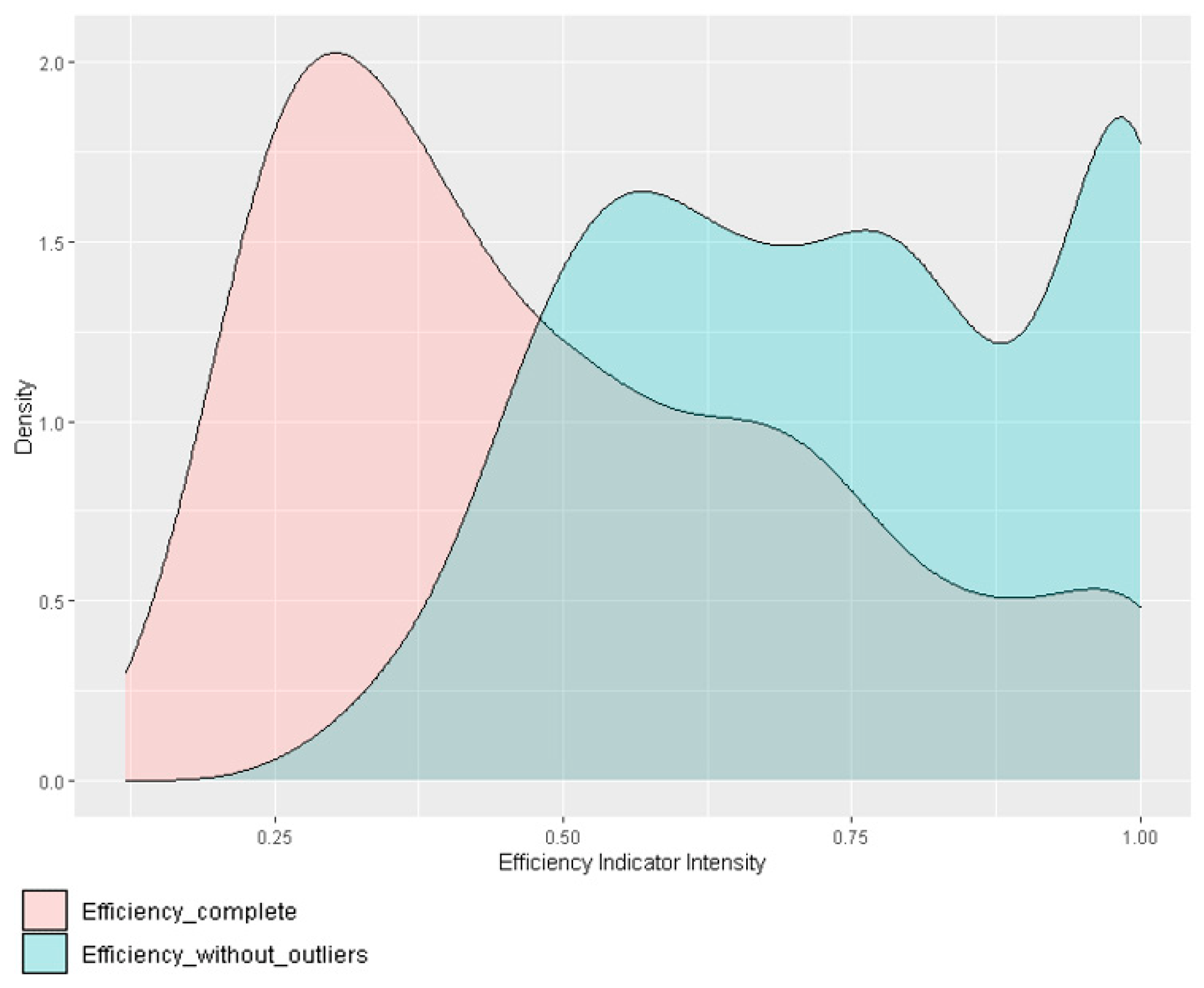
2.3. Detection of Influent Observations in Eco-Efficiency Calculations

According to Wilson [9], the DEA requires a prior procedure of data cleansing before estimating indices. As deviations in relation to the frontier implies inefficiency, the point values of DEA efficiency are strongly affected by both the measurement errors and the presence of outliers. The atypical DMUs bias the efficiency indices of the other DMUs downwards. In this context, Bogetoft et al. [33] suggest an initial exploratory data analysis using the multivariate data cloud method. However, this procedure requires several steps, and for very large samples, there can be computational capacity constraints.

Another approach to handle outliers in large samples is the jackstrap method, proposed by Sousa et al. [34], which combines bootstrap and jackknife methods. This approach uses a leverage concept and seeks to estimate the impact of atypical DMUs on efficiency measures. It assumes that the most influential DMUs exhibit well-above-average leverage. Thus, the leverage is associated with the impact of removing a DMU on the efficiency scores of the remaining DMUs. This leverage shifts the efficient frontier when a given DMU is taken from the analysis.

The procedure of Sousa et al. [34] can be summarized as follows: (i) randomly select, through the use of bootstrap without replacement, a fraction (10% to 20%) of the original sample, consisting of K DMUs, called an artificial bubble; (ii) estimate the efficiency of the K DMUs, before and after the removal of each $DM{U}_j$ one by one; (iii) calculate the leverage of the j-th DMU through the Equation (6); (iv) repeat B times the previous steps, accumulating the leverage values in a subset ${\check{l}}_{jb}$ for all randomly selected DMUs, where b = 1,…, B; (v) compute the average leverage of each DMU $\left({\overline{l}}_j\right)$ and the global average leverage ($\tilde{l})$; (vi) order the DMUs according to their respective average leverages and determine the cut-off point beyond which all DMUs with leverage greater than or equal to this point can be considered outliers. For this purpose, the method uses two criteria: the Kolmogorov–Smirnov test (K-S) and the Heaviside function (step function), which take into consideration the sample size.

$$l_j=\sqrt{\frac{{{\displaystyle \sum }}_{k=1,k\ne j}^n {\left({\theta }_{ki}^{-}-{\theta }_k\right)}^{2 }}{n-1}}$$

(6)

where ${\theta }_k$ (to k = 1,…, K) is the set of efficiency indicators before the removal of the DMU_j, and ${\theta }_{ki}^{-}$ (to k = 1,…, K; k $\ne j)$ is the set of efficiency indicators after the removal of the DMU_j.

2.4. The Bootstrap to Estimate the Bias and the Confidence Interval

After identifying and excluding the outliers, we estimate the bias and the confidence interval, following Simar et al. [32]’s special technique called “ smooth homogeneous bootstrap”, differing from the “classical naive bootstrap”, which is inconsistent in the inference of DEA indicators.

We use a version of the homogeneous smoothing algorithm used in the R function boot.sw98 of the FEAR package [35] to estimate the output-oriented Shephard efficiency that can be summarized as follows [32]:

• For each DMU (x_i, y_i) ∈ S_n, compute the efficiency ${\widehat{\theta }}_i$ using the DEA model chosen—CRS (3) or VRS (5)—and transforming the Farrell efficiency into Shephard efficiency;
• Generate a random sample of size n of ${\widehat{\theta }}_i$ using a density function of kernel smoothing and the reflection method to obtain ${\widehat{\theta }}_1^{*},\dots , {\widehat{\theta }}_n^{*}$, where ${\widehat{\theta }}_i^{*}$ is the bootstrap score of the DMU_i. It is done as follows:
  • Extract a sample with replacement of (${\widehat{\theta }}_1$,…, ${\widehat{\theta }}_n$) and call the results (${\beta }_1$,…, ${\beta }_n$);
  • Calculate the bandwidth h and generate independent random numbers of standard-normal distribution: ${ϵ}_1$,…, ${ϵ}_n$;
  • Compute

    $${\tilde{\theta }}_i=\{\begin{array}{c}{\beta }_i+h{ϵ}_i if {\beta }_i+h{ϵ}_i\le 1 \\ 2-{\beta }_i-h{ϵ}_i otherwise\end{array} thus {\tilde{\theta }}_i\le 1$$

    (7)

Adjusting ${\tilde{\theta }}_i$ obtains the parameters with the correct asymptotic variance, calculating

$${\widehat{\theta }}_i^{*}=\overline{\beta }+\frac{1}{\sqrt{1+h^2/{\widehat{\sigma }}^2}}\left({\tilde{\theta }}_i-\overline{\beta }\right)$$

(8)

where the variance ${\widehat{\sigma }}^2=\frac{1}{n}{{\displaystyle \sum }}_{i=1}^n{\left({\widehat{\theta }}_i-\overline{\widehat{\theta }}\right)}^2$ and $\overline{\beta }=\frac{1}{n}{{\displaystyle \sum }}_{i=1}^n{\beta }_i$

3.

Extract a new sample data $S_n^{*}$ whose elements, Y^* = [${\mathit{y}}_1^{*}$, …, ${\mathit{y}}_n^{*}$] and X^* = [${\mathit{x}}_1^{*}$, …, ${\mathit{x}}_n^{*}$], are given by ${\mathit{y}}_i^{*}={\mathit{y}}_i\frac{{\widehat{\theta }}_i^{*}}{{\widehat{\theta }}_i}$ e ${\mathit{x}}_i^{*}={\mathit{x}}_i$. That way, ${\mathit{y}}_i^{*}$ will continue in the same radius as ${\mathit{y}}_i$;

4.

Use the DEA model chosen—(3) or (5)—to calculate the estimation of new indices ${\widehat{\theta }}_i^b$ de $\left({\mathit{x}}_i^b, {\mathit{y}}_i^b\right)$;

5.

Repeat the steps 2, 3 and 4 B times to obtain the set of estimations [${\widehat{\theta }}_1^b,\dots ,$ ${\widehat{\theta }}_n^b$] to b = 1… B.

The distribution of the set ${\left\{{\widehat{\theta }}_i^b\right\}}_{b=1}^B$ provides a consistent estimation of the real efficiency indicator of the DMU_i, this consistency being higher when B→∞ and n→∞. Simar et al. [32] recommend at least 2000 samples to get adequate results, although higher numbers represent more accurate indices.

As highlighted by Simar et al. [32], when the bootstrap is consistent, the difference between initial efficiency (${\widehat{\theta }}_i$) and the mean bootstrap efficiency should be similar to the difference between the initial efficiency and the real efficiency (${\theta }_i$) for a certain DMU_i. Thus, the bias for each DMU_i can be expressed following the equation:

$${\widehat{bias}}_i=\frac{1}{B}{\displaystyle \sum }_{b=1}^B{\widehat{\theta }}_i^{*}-{\widehat{\theta }}_i={\overline{\widehat{\theta }}}_i^{*}-{\widehat{\theta }}_i$$

(9)

where ${\overline{\widehat{\theta }}}_i^{*}$ is the average of the B estimations of the bootstrap efficiency of the DMU_i.

So, the estimator of ${\widehat{\theta }}_i$ correcting the bias is:

$${\tilde{\theta }}_i={\widehat{\theta }}_i-{\widehat{bias}}_i={\widehat{\theta }}^i-{\overline{\widehat{\theta }}}_i^{*}+{\widehat{\theta }}_i=2{\widehat{\theta }}_i-{\overline{\widehat{\theta }}}_i^{*}$$

(10)

However, for Simar and Wilson (1998), the correction of the bias should not be used, except when:

$${\widehat{\sigma }}^2<\frac{1}{3}{\left[{\widehat{bias}}_i\right]}^2$$

(11)

where ${\widehat{\sigma }}^2$ is estimated with the bootstrap estimators’ variance, so that:

$${\widehat{\sigma }}^2=\frac{1}{B}{{\displaystyle \sum }}_{b=1}^B{\left[{\widehat{\theta }}_i^b-\frac{1}{B}{{\displaystyle \sum }}_{b=1}^B{\widehat{\theta }}_i^b\right]}^2$$

(12)

Once the empirical distribution of the bootstrap and the bias efficiency is known, we can find the confidence intervals with a significance level (1–α), calculating the critical values a_α and b_α, so that:

$$Pr\left[-b_{\alpha }\le {\widehat{\theta }}_i^{*}-{\widehat{\theta }}_i\le -a_{\alpha }\right]\approx Pr\left[-b_{\alpha }\le {\widehat{\theta }}_i-{\theta }_i\le -a_{\alpha }\right]\approx 1-\alpha$$

(13)

In order to estimate a_α and b_α, Simar et al. [31] suggest the use of a percentage process. This process is associated with the bootstrap estimators ordination from the highest to lowest and the elimination, on both extremes of this ordination, of the percentage (α/2) of the values, leading to an estimated interval:

$${\widehat{\theta }}_i+a_{\alpha }\le {\theta }_i\le {\widehat{\theta }}_i+b_{\alpha }$$

(14)

This procedure is applied to the other DMUs that form the original sample.

2.5. Testing for Return-to-Scale Types

According to Simar at al. [36], defining a priori assumptions about returns to scale can seriously distort the efficiency measures if the original technology is different. For model development and validation, it should be tested if the technology T, from which observations are sampled, presents a constant return to scale or not. Simar et al. [36] formalized the following test: the null hypothesis (H₀) is that T is CCR, or the alternative hypothesis (H_a) is that T is BCC.

The test is based on the observation of the relation ${\widehat{\theta }}_{CCR}/{\widehat{\theta }}_{BCC}$ in each DMU, indicating the scale efficiency ${\widehat{\theta }}_s$. As the ${\widehat{\theta }}_{BCC}$ ≥ ${\widehat{\theta }}_{CCR}$, so ${\widehat{\theta }}_s\le 1$. If ${\widehat{\theta }}_s=1$ to all DMUs, the technology is CCR. If there were many DMUs where ${\widehat{\theta }}_s<1$, there is evidence that the technology is BCC. To estimate those technologies and the scale efficiency using random variables, the null hypothesis should be rejected if the scale efficiency indices estimated ${\widehat{\theta }}_s$ are significantly smaller than 1, i.e., if the ${\widehat{\theta }}_s$ estimated are lower than a critical value. Thus, we should focus on finding the distribution of ${\widehat{\theta }}_s$ and calculating the critical value, $c_{\alpha }$.

Simar et al. [36] suggest the use of the statistic:

$$S=\frac{{{\displaystyle \sum }}_{i=1}^n{\widehat{\theta }}_{i,CCR}}{{{\displaystyle \sum }}_{i=1}^n{\widehat{\theta }}_{i,BCC}}$$

(15)

Since S ≤ 1, if S is close to 1, H₀ should not be rejected, and, if S is significantly lower than 1, H_a should be accepted. Thus, H₀ is rejected when S < $c_{\alpha }$ based on a given significance level.

Since the distribution of the population values of S is unknown, it is not possible to determine $c_{\alpha }$ directly. Simar et al. [36] recommend using the bootstrap method to estimate the distribution of this parameter. The algorithm obtains the efficiency bootstrap set to the model CCR, the bootstrap set to the model BCC and the bootstrap distribution of S. This procedure allows the comparison of the estimated value of S given by (13) and the critical value related to the significance level to make a decision about H₀.

2.6. Eco-Efficiency Dependency of External Factors: Second-Stage Analysis

After estimating the confidence intervals of the eco-efficiency and testing the hypotheses to technologies, the following questions are relevant: why are some DMUs more eco-efficient than others? Which exogenous factors determine eco-efficiency?

The interest awakened by these questions led to the emergence of the procedure commonly entitled “two-stage analysis” [3]. In the first stage, the eco-efficiencies are calculated. In the second stage, the analysis focuses on identifying the influence of variables contextual (Z) on the eco-efficiency of DMUs. Lovell [37] suggests the use of variables under the control of the manager in the first stage and variables that the producer does not control in the second stage. Therefore, the variables Z are called exogenous, contextual, or non-discretionary variables and can be internal or external to the production process.

The addition of exogenous variables is pertinent, as the number of the external influential factors is not small. Furthermore, their effect over the efficiency can be higher than that produced by the variables controlled by the managers. This analysis makes it possible to discover if the producer classified as inefficient really is so or if, even doing everything possible, there are uncontrolled factors that do not allow it to achieve the results that others can.

In order to analyze whether Z explains the corrected efficiency, one can use regression models. However, DEA indices show autocorrelation (serial correlation) and are truncated, and there is often multicollinearity in the contextual variables. Therefore, the basic assumptions of the regression model are violated, and, therefore, biased results can be generated [38].

Simar et al. [11] propose the application of a truncated regression model (tobit or equivalent) with bootstrap in order to overcome these disadvantages. The tobit method, estimated by maximum likelihood, can be used when the dependent variable is limited between ranges of values. In the regression, defined by ${\tilde{\theta }}_i={\mathit{Z}}_i\mathbf{\beta }+{\epsilon }_i$, ${\tilde{\theta }}_i$, the corrected efficiency, is estimated in the first stage; ${\mathit{Z}}_i$ corresponds to the vector of explanatory variables that could influence the efficiency indicators through the parameters vector $\mathbf{\beta }$. The vector ${\epsilon }_i$ is the noise or the random error associated with each DMU, associated with the inefficiency part not explained by ${\mathit{Z}}_i$. Assumptions relate to ${\epsilon }_i$ following a normal distribution with average 0 and variance ${\sigma }_{\epsilon }^2$ censored between 0 and 1.

Simar et al. [11] suggest two algorithms to incorporate of the bootstrap in a truncated regression model. Using a Monte Carlo experiment, the authors examine and compare the performance of those two algorithms and demonstrate that both overcome the conventional regression methods (tobit and truncated regression without bootstrap). For samples with less than 400 units, the proposed Algorithm #1 adjusts better than Algorithm #2, which is more efficient from samples that exceed 800 units. As the sample used is closer to 400, it is adapted to Algorithm #1, which is described below, following [11]:

• Estimate the corrected efficiency ${\tilde{\theta }}_i$ to all DMUs (i = 1, …, n) using the DEA-CRS or DEA-BCC model oriented to outputs;
• Regress ${\tilde{\theta }}_i={\mathit{Z}}_i\mathbf{\beta }+{\epsilon }_i$, using a tobit regression using maximum likelihood estimation, aiming to obtain estimations $\widehat{\mathbf{\beta }}$, $\widehat{\epsilon }$ and its standard deviation, ${\widehat{\sigma }}_{\epsilon }$;
• Repeat the next three steps (a, b, c) L times to produce a set of bootstrap estimators ${\left\{{\widehat{\beta }}^l,{\widehat{\sigma }}_{\epsilon }^l\right\}}_{l=1}^L$:
  • For each DMU_i, with the ${\widehat{\sigma }}_{\epsilon }$ estimated in stage 2, extract random values of $e_i$ of a normal distribution N(0,${\widehat{\sigma }}_{\epsilon }$) truncated to left in (1 − ${\mathit{Z}}_i\widehat{\mathbf{\beta }}$);
  • For each DMU_i estimate ${\tilde{\theta }}_i^{*}$ $={\mathit{Z}}_i\widehat{\mathbf{\beta }}+e_i$, where $\widehat{\mathbf{\beta }}$ is the estimator found in stage 2;
  • Following the maximum likelihood estimation, estimate the truncated regression of ${\tilde{\theta }}_i^{*}$ in ${\mathit{Z}}_i$ obtaining the estimations ${\widehat{\beta }}^{*},{\widehat{\sigma }}_{\epsilon }^{*}$;
• Use the L values of the set ${\left\{{\widehat{\beta }}^l,{\widehat{\sigma }}_{\epsilon }^l\right\}}_{l=1}^L$ to construct the confidence intervals of $\beta$ and ${\sigma }_{\epsilon }$.

2.7. Object of the Study and Variables

We focus this study on the municipal agriculture eco-efficiency in the Brazilian Amazon biome, an ecosystem of worldwide relevance. This region represents 60% of the Amazon rainforest, which also includes the territories belonging to nine South American nations, and represents more than half of the remaining tropical rainforests on Earth. The region contains the biggest biodiversity in a tropical rainforest and 20% of the fresh water of the world. The Brazilian Amazon rainforest covers around 4.2 million km² (49.29% of the national territory), where 25 million people live in 552 counties located in the following states: Acre (AC), Amazonas (AM), Amapá (AP), Mato Grosso (MT), Maranhão (MA), Pará (PA), Rondônia (RO), Roraima (RR) and Tocantins (TO). From the earliest deforestation in the 18th century to July 2019, the total area deforested in this region amasses a 719,014 km² of surface, which corresponds to 17.1% of its total area [39].

According to the 2017 Agricultural Census of IBGE (2019) [19], in the region, there are 677,596 agricultural establishments, of which 90% are small farmers. These establishments generate annual revenues of BRL 68,417 billion (equivalent to USD 20,852 billion) and occupy an area of 97,655,962.00 ha. A large part of this area is covered by native vegetation given the requirement of owners maintaining 80% of legal reserve, in compliance with the Brazilian Forest Code for this region.

In order to estimate the eco-efficiency of 552 municipalities (DMUs), we consider in the first stage the classic inputs and products used in the literature, adding three environmental externalities as outputs [40]. The inputs of the model are: x₁—establishments area in hectares, x₂—machines, measured by the proxy annual cost with fuels and lubricants in thousands of Brazilian reais, x₃—annual expense with inputs to plant and animal production in thousands of Brazilian reais, x₄—labor force filled in the establishments (paid and familiar), x₅—other costs in thousands of Brazilian reais; as outputs, y₁—annual gross revenue in 10 million Brazilian reais. Among the externalities, one positive (y₂) and two negative (y₃ and y₄) were chosen: y₂—area of natural woods and forests grown in the establishment in 10 thousands hectares, which represents a proxy of environmental services provided by nature in this area; y₃—biodiversity impact index of agriculture, calculated by the Shannon index (SHDI) (The Shannon index is a proxy used in the eco-efficiency literature to estimate the impact of farming on biodiversity [41]. It is calculated for each county i using $y_i=1/e^{SHDI}$, where $SHDI=-{{\displaystyle \sum }}_{c=1}^C\left(s_{ci}· ln s_{ci}\right)$, $s_{ci}=Are{a}_{ci}/Are{a}_i$, considering the number of cultures (c) of a county and its relative weight (s_ci). Thus, the pressure in the biodiversity can assume values between 0 and 1. A value equal to the unit represents establishments that produce only one type of culture, causing a higher negative impact on biodiversity. A value close to zero indicates a lower impact on the flora and fauna of the ecosystem. (y₄—annual greenhouse gas emissions by the agricultural sector in millions of tons of GWP—AR5 (Global Warming Potential, according to conversion factors based on the Fifth Assessment Report of the IPCC)). The last two variables were inverted so that, when maximizing the production vector, these negative externalities are minimized. We extract and calculate the inputs and outputs based on information by municipality from the 2017 Agricultural Census, with the exception of y₄, which was downloaded from the Greenhouse Gas Emission and Removal Estimating System (SEEG) website (https://seeg.eco.br/o-que-e-o-seeg, accessed on 1 May 2021).

In order to investigate the association of exogenous factors with eco-efficiency in the second stage, we selected 9 variables, considering the variables found in the literature [13,42], and available in the Census. We also included other variables not covered in the mainstream literature, aiming at performing an exploratory analysis. The variables of the second stage are: z₁—the percentage of the establishments classified as familiar farming; z₂—the percentage of establishments that received technical assistance; z₃—the percentage of owners associated with the cooperative; z₄—the percentage of establishments whose producer has at least a high school degree, a proxy of education level; z₅—the percentage of establishments whose producer is the landlord; z₆—the percentage of establishments that obtained financing from banks; z₇—the population density of the municipality (people/km²), a proxy of the market size; z₈—the latitude; and z₉—longitude. These last two variables represent the geographic coordinates of the municipality location, and they will allow the identification of the spatial location impact in the eco-efficiency.

3. Results and Discussion

3.1. Descriptive Analysis, Outlier Detection and Final Sample

Aiming at providing an overview of the initial sample (552 municipalities), we present the key descriptive statistics of inputs, outputs and environmental variables in

Table 1. Descriptive statistics of the inputs (x), products (y) and environmental determinants (z).

	Mean	Median	Standard Deviation	Minimum	1° Quartile	3° Quartile	Maximum
x1	176,913	89,392.5	250,039.1	72	29,453	220,394	2,462,092
x2	5947.399	2280	11,922.16	1	663.8	6217.8	122,958
x3	27,865.48	5704.5	82,192.97	32	1132	18,530	1,004,087
x4	4500.781	3338.5	4337.971	105	1825	5774	48,246
x5	37,807.83	11,388	97,494.70	23	2542	32,924	1,320,992
y1	12.39416	4.83375	26.95020	0.0857	1.65	11.16	306.1954
y2	6.772156	2.4825	11.13849	0.00001	0.650	7.785	96.2598
y3	2.320974	1.64081	1.728685	1.00084	1.180	2.862	13.99893
y4	83.67418	7.29497	384.8253	0.23926	2.697	35.992	6681.91
z1	0.798722	0.814445	0.1154	0.27478	0.740	0.8725	0.980769
z2	0.130973	0.090833	0.1290	0	0.040	0.170	0.898204
z3	0.047284	0.020535	0.0691	0	0.010	0.060	0.562325
z4	0.216148	0.200064	0.0935	0.02521	0.140	0.270	0.65
z5	0.795039	0.859133	0.1927	0.055172	0.710	0.930	1
z6	0.113395	0.091004	0.0884	0.002396	0.050	0.160	0.754491
z7	31.71617	6.799077	163.2888	0.031568	2.345	18.942	2803.911
z8	−5.9986	−4.40389	4.7996	−26.7836	−9.987	−2.245	4.595012
z9	−53.6487	−51.2433	7.4920	−72.8958	−59.70	−47.61	−36.4

Source: elaborated by the authors.

. The table shows a wide dispersion of the data. Moreover, for most variables, the minimum values are well below the first quartile, and the maximum are well above the third quartile, indicating the existence of significant heterogeneity in the data and the evidence of potential extreme observations, i.e., outliers.

The presence of outliers and data heterogeneity can be explained by the large difference in the adoption of good practices in agriculture and the great number and technological diversity of rural properties but also by possible problems of errors or omissions in the data, especially those resulting from the self-declaratory system of the Agricultural Census. These data-gathering problems should affect the eco-efficiency indicators, considerably undervaluing estimations. Therefore, to ensure the reliability of the found indices, it is important to make some adjustments to reduce the impact of those problems.

In order to avoid these problems, we use the jackstrap (available as an R package in https://CRAN.R-project.org/package=jackstrap (accessed on 8 May 2022)) method for the detection of outliers [43]. The application of this method selected bubbles that contained 10% of the total number of DMUs and 2000 bootstrap replications and calculated the average leverage in each DMU, as well as the value threshold with two basic models: DEA-CRS and DEA-VRS. The jackstrap method for DEA-CRS found 25 and 13 outliers for the criteria of the Heaviside function and the Kolmogorov–Smirnov test (K–S), respectively. For DEA-VRS, the method detected 20 and 15 outliers of the Heaviside function and the K–S test. Among these options, we decided to use the strictest criterion, choosing the Heaviside function of the DEA-CRS.

A detailed analysis of the records of the 25 DMU outliers found that these units had low values for certain inputs or high values for certain products. In this context, some of these DMUs are able to increase their inputs several times and continue to be eco-efficient. This outcome is very unlikely, because it is verified that the technological levels of these municipalities are not very far from the average found in the region, unless these differences represent errors in the data. For example, we have the case of Anajás (PA), which reported a super-efficiency index [44] with a CRS of 5.55, indicating that it can increase its resources by more than 450% and still remain in the eco-efficiency frontier.

Figure 1 shows the density curves of the eco-efficiency obtained through the DEA-CRS model applied before and after the removal of the 25 DMUs of major leverage. It is noticed that the removal of outliers generates a great impact on the distribution of the computed eco-efficiency scores. The new distribution indicates a higher mean and median and a shift to the region of higher eco-efficiency, indicating that the original efficiency scores are biased downwards due to the existence of outliers.

It is important to notice that the number of DMUs removed represent less than 4.5% of the original sample and 48% of them are found in the State of Pará. Thus, from hereinafter, we present results of a sample of 527 (=552 − 25) DMUs.

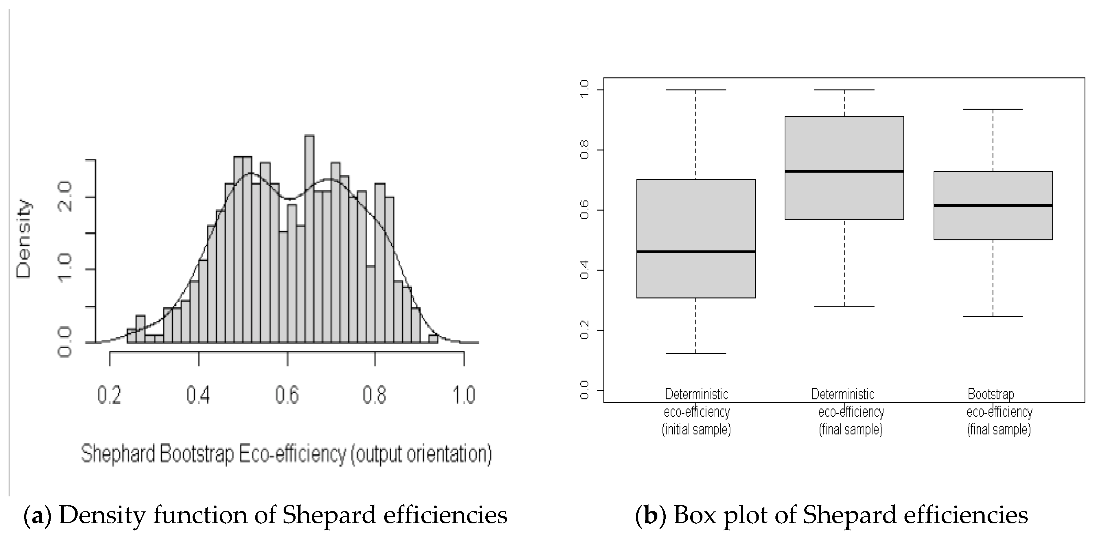
3.2. Statistical Inference of the DEA Indices

Taking into account the sample without the outliers, the significance test of return to scale is carried out, since the arbitrary choice of the technology can result in inappropriate conclusions. According to the described method, this test was performed using the distribution of eco-efficiency scores CCR and BCC obtained from the bootstrap with 2000 samplings. The test has the null hypothesis (H₀) that T is CCR and the alternative hypothesis (H_a) that T is BCC. The H₀ should be rejected if S (Equation (15)) was significantly lower than the critical value to $\alpha =0.05$.

Since the estimated value of S = 0.9577 is higher than the critical value $c_{\alpha }$ = 0.9210, the null hypothesis cannot be rejected. The results obtained also show an error type I equal to 0.448 (superior to $\alpha$), indicating that it is possible to make a mistake with a probability of 44.8%, if the null hypothesis were rejected, based on this estimation. As a consequence, it is possible to state that the technology T shows constant returns to scale. Thus, different sizes of counties (small, medium and large) can be equally eco-efficient.

In the empirical literature, this result is controversial. It is in dissonance with the evidence obtained by Souza at al. [14], which rejects the hypothesis of constant returns to scale in the technical efficiency analysis of 4964 Brazilian counties. However, the findings confirm the results of Freitas et al. (2019) [45], who found the possibility of efficiency in properties of all sizes. The data used in both works are from the 2006 Agricultural Census.

If the municipality is considered as a productive unit, the result brings to light the old debate about the long-term sustainability of different sizes of property. It motivates the questioning of the hypothesis that, in a market of perfect competition, in the long term, small companies will tend to disappear, since their production scales do not allow them to operate at the minimum-unit-cost level.

As indicated by Alves [46], the existence of convergence on a small number of large farms is not compatible with the existence of competitive markets, and it contradicts the observed world. For this reason, the author argues that the results of models that detect this tendency should make researchers inquire which market imperfections underlie this convergence.

The high inequality in the distribution of land tenure in the studied region and in Brazil in general is widely recognized. However, when computing the Gini index to measure inequalities in land distribution, Hoffmann [47] shows that, in the last five censuses (from 1975 to 2017), the Brazilian land tenure structure remained quite stable, with a Gini index around 0.86. Thus, for this author, in this period, there is no significant upward or downward trend for the values of the average and median areas, as well as for the number of establishments. Therefore, despite the existence of a series of imperfections in the Brazilian market [48], the thesis that size is not a condition for a company to be eco-efficient and the existence of constant returns to scale (CRS) can be supported.

In addition, this result is consistent with some theoretical studies consulted. As observed by Caves et al. [49] and Porter [50], small businesses can be competitive if they efficiently find their market niche and seize their flexibility and capacity for innovation, as, for example, in organic farming and in supplies for local markets.

After accepting CRS technology, we continue by estimating the Shephard eco-efficiency score oriented to the outputs and its confidence intervals, considering the random bias inherent in the data. We use the Simar et al. [31] procedure (available at the FEAR library website: https://pww.people.clemson.edu/Software/FEAR/fear.html (accessed on 9 May 2022)), described in Section 2. The result with 2000 samplings has enabled the setting of a stochastic production frontier that should be very close to the real one, as well as to estimate the corrected eco-efficiency indicators. However, due to the database size, only the five most eco-efficient counties and the five most eco-inefficient are depicted (

Table 2. CRS Shephard eco-efficiency oriented to the output and the confidence interval (95%).

DMU	Without the Outliers and with Bias Correction	Confidence Interval		Without the Outliers and without Bias Correction	With the Initial Sample
		Lower Limit	Upper Limit
Parauapebas (PA)	0.936	0.910	0.983	0.998	0.450
Novo Airão (AM)	0.897	0.861	0.973	0.985	0.847
Medicilândia (PA)	0.891	0.869	0.938	0.953	0.506
Presidente Figueiredo (AM)	0.885	0.856	0.971	0.977	0.852
Rio Preto da Eva (AM)	0.880	0.858	0.985	1.000	0.849
Santa L. do Paruá (MA)	0.274	0.259	0.304	0.308	0.178
Garrafão do Norte (PA)	0.268	0.255	0.330	0.334	0.215
Anajatuba (MA)	0.267	0.261	0.299	0.303	0.121
Governador Nunes F. (MA)	0.255	0.244	0.288	0.291	0.128
Itapecuru Mirim (MA)	0.247	0.238	0.275	0.278	0.137
Average	0.615	0.601	0.720	0.730	0.519

Source: formulated by the authors.

). In order to compare these results, we add to Table 2 the previously estimated scores.

Table 2 shows that, in the studied region, there are relevant eco-inefficient behaviors. For example, the municipality of Parauapebas (PA) was the best positioned in the corrected eco-efficiency ranking. Even so, the ratio of the output vector (y) by the scalar represents the eco-efficiency index of (y/0.936), reveals the possible improvements and gives the optimal level of production without modifying its inputs. The same metric can be calculated for other municipalities. The aggregated values indicate that it is possible to increase, throughout the studied region, the annual revenue by 50.17% and the preserved areas by 54.06% and, at the same time, to reduce the impact on the biodiversity index by 21.4% and the GHG emissions by 37.15%.

The results of Table 2 also indicate that the global average was of 0.615, but the eco-efficiency averages among the counties vary from one state to another. The state with the highest average was Amapá with a score of 0.72, followed by Acre (0.70), Roraima (0.699), Mato Grosso (0.697), Amazonas (0.665), Pará (0.63), Tocantins (0.566), Maranhão (0.528) and Rondônia (0.513).

In Table 2, it is possible to observe the confidence intervals. These indicate that corrected indices can be statistically equal, since, if two intervals intersect, it would be possible to affirm that these DMUs do not have different levels of eco-efficiency. This is the case of the first five municipalities in the ranking. The result shows that great caution should be exercised when performing comparative analyses between DMUs.

Furthermore, it is noted that the eco-efficiency indices corrected for bias are generally higher than the indices of the original sample and lower than the indices with the final sample (without the outliers). This evidence suggests that the deterministic scores of the final sample must be overestimated and those of the initial sample underestimated.

This argument is supported by Figure 2. Figure 2a depicts the density curve of the corrected eco-efficiency indicators, indicating that is very different from the curves of the deterministic eco-efficiency scores before and after the removal of the outliers represented in Figure 1. Thus, the probability of each eco-efficiency range of values differs in each model. Figure 2b displays the boxplots of the three distributions, indicating that the medians, means and dispersions of the indices are different. The means and median of the corrected indices are situated between the mean and median of other distributions, having a lower interquartile range. This result suggests that the indices generated by the bootstrap procedure, with their corresponding confidence intervals, are more efficient and robust.

We also conduct tests of comparison of distributions. The ANOVA and Kruskal–Wallis tests indicated that there are significant differences between the distributions. Post-hoc tests also confirm that there is a significant difference between the pairwise distributions. This finding highlights the relevance of performing bootstrap analysis when estimating efficiency indices with DEA.

However, the eco-efficiency indicators obtained in this stage can only be considered compelling if all of the counties are operating with the same background. This is not evident when the values of the background variables shown in Table 1 are observed. So, it is necessary to embody these variables into the eco-efficiency analysis.

3.3. Impact of the Contextual Variables into Eco-Efficiency Indicators

The influence of environmental factors on the output-oriented Farrell CRS eco-inefficiency corrected indices, which are, in this case, greater than or equal to 1, was estimated following the second-stage algorithm of [11], using the R FEAR Package.

Table 3. Results of the model applied to second-stage estimations.

Environmental Variables	Beta Coefficient	Confidence Interval of 95%		Average Marginal Effect
		Lower Limit	Upper Limit
Y-intercept	2.2547	2.25	2.26
z1—familiar farming	0.1219	0.11	0.13	0.12185
z2—technical assistance	−0.4800	−0.49	−0.47	−0.48002
z3—cooperative	−0.0892	−0.10	−0.08	−0.08918
z4—high school	−0.6851	−0.69	−0.68	−0.68505
z5—landlord	−0.0340	−0.04	−0.03	−0.03400
z6—financing	1.1557	1.15	1.17	1.15569
z7—density	0.00004	0.00003	0.00004	0.00004
z8—latitude	0.00024	0.00007	0.00042	0.00024
z9—longitude	0.0084	0.00830	0.00850	0.00840
Error variance	0.398	0.398	0.398

Source: formulated by the authors.

presents the results of the tobit regression with 2000 bootstrap resamplings. As the estimated coefficients (betas) of the variables do not have a direct interpretation equal to the linear models, the average marginal effect on eco-efficiency is included.

According to these results, all background variables are different from zero and significant at the 5% level. However, three of them, having values very close to zero, affect irrelevantly the eco-inefficiency. They are variables associated with: z₇—demographic density of the county, a proxy of the market size; z₈—latitude; and z₉—longitude. The poor significance of these last two variables indicates, unexpectedly, that spatial location has little importance to eco-efficiency.

The variable z₆—financing has the highest level of influence. However, this variable presented an unexpected signal, according to the theory, and it can indicate a serious market failure. The average marginal effects in Table 3 express that an increment of 1% in the numbers of establishments with financing increases the value predicted in the eco-inefficiency of the counties by 1.15 points.

This fact, even if is not unanimous, has already been shown by several researchers. In the 1980s, Taylor et al. [51], while studying growers in the state of Minas Gerais in Brazil, found that financing had a slightly negative effect in the allocative efficiency and in technical efficiency. Souza et al. [14] also obtained an unexpected beta coefficient to this variable, following Algorithm #1 and #2 of [11] in the efficiency analysis of 4964 Brazilian counties with data from the 2006 agricultural census. It can be explained by the politics of subsidized credit, which encourage the purchase of inputs and machinery at an inefficient price, reducing the allocative efficiency [52]. Araújo et al. [53] concluded that the subsidized credit of the National Program for Strengthening Family Farming (PRONAF) imposes a selection bias and does not stimulate the productive diversification, which compromises the promotion of development and the reduction of rural poverty.

The second variable with a greater impact is the educational level of managers. The average marginal effects in Table 3 show that the increment of 1% in the number of establishments whose manager has at least a high school degree may reduce the eco-inefficiency indicator in 0.6851 points. Furthermore, it indicates that rural managers with better training can have the expertise to assign more importance to economy and environmental issues, as well as in the management of the activities and in the selection of new technologies. This result corroborates other research outcomes [54,55]. For Fernandes et al. [52], rural managers, like any other managers, make better decisions when they are better prepared.

Another relevant factor to explain the differences observed in the eco-efficiency indicators is technical assistance. Table 3 indicates that the average marginal effect in the eco-inefficiency is −0.48002. This fact can be explained by the evidence that, when receiving technical assistance, the producers tend to correct the problem of inadequate use of inputs and also those related to what, how much and how to produce with less environmental impact. The result is supported by the study of Gomes et al. [56], which confirms the existence of a positive relationship between the time in which the producers receive technical assistance and the efficiency indicators. Braga et al. [57] also show that the extensionist services impacted positively the income of the rural producers by 19%, considering that the private technical assistance presented a higher impact than the public rural extension.

In Table 3, an addition of 1% in the number of properties classified as familiar agriculture increases eco-inefficiency by 0.12185 points. This fact can be related to the low level of education of the producers and the low technological diversity and specialization of work in the properties of this category. Usually, the family has the role of owner, manager and producer and is also responsible for all production, marketing and logistics.

This result is partially consistent with the findings of the pertinent empirical literature. However, it does not disagree with the previously stated argument about the possibility of the small property (not necessarily of the family type) being as competitive as the large ones. Thus, public policy needs to gather initiatives that provide to familiar farms chances to compete on equal terms with large farms, especially regarding the prices paid by inputs and products’ sale prices [48,58].

Table 3 also depicts a significant relation between eco-efficiency and cooperativism, which is very rare in the region. As observed by Ramos et al. [58], a cooperative provides strong chances for the enhancement of eco-efficiency, since the collective productive arrangements improve access to information, making it easier to compare the results and replicate sustainable good practices. The cooperative allows farmers to enhance extension services and technical assistance, to raise their bargaining power in the marketing of products and the acquisition of inputs and to lessen the indivisibility of the high cost means of production (for example, harvesters and silos).

Finally, our study shows that land property is another relevant factor in the reduction in eco-inefficiency, although the impact is small (−0.034). This result is remarkable in face of the recurring illegal appropriation of public land, denominated squatting. In these irregular areas, the development of agricultural or forestry activities infringe environmental, agrarian, civil and tributary regulations [59]. In addition, they create uncertainty about the landholding status, causing social conflicts (especially with indigenous communities) and obstructing the implementation of conservation and economic development projects in the region [59].

4. Conclusions

In this study, we estimated robust agricultural eco-efficiency scores among 527 municipalities in the Amazon biome, pointing out how much it is possible to maximize economic and environmental objectives, having as a reference the best practices in the region. We use the jackstrap method to identify and eliminate outliers that affected the efficiency levels. Then, using bootstrap techniques, we perform significance tests for returns of scale. Once the CRS technology was confirmed, we estimated the score corrected for the random bias inherent in the data sample. Furthermore, as the estimated scores are also affected by exogenous factors not considered in the eco-efficiency calculations, we apply bootstrapped tobit truncated regression models to investigate how these environmental variables influenced these scores. The study indicates the compatibility between economic growth and environmental preservation in the Amazon biome and that eco-efficiency scores are significantly impacted by exogenous factors. In this context, we fill an important gap regarding the evaluation of the environmental economic performance of agriculture in one of the most vulnerable biomes in Brazil.

Finally, we argue that the current analysis could be complemented by examining the dynamics of eco-efficiency indicators over time, identifying the dynamics of efficiency in the sector. Therefore, the natural extension of the investigation would be to include panel data in the analysis. This will be the subject of future research, as it is another gap found in the literature.

References

1. Araujo, R.D.C.; Ponte, M.X. Agronegócios na Amazônia: Ameaças e oportunidades para o desenvolvimento sustentável da região. Rev. Ciênc. Agroambient. 2015, 13, 101–114. [Google Scholar] [CrossRef]
2. Fishlow, A.; Filho, J.E.R.V. Agriculture and Industry in Brazil; Columbia University Press: Chichester, NY, USA, 2019. [Google Scholar] [CrossRef]
3. Emrouznejad, A.; Yang, G.-L. A survey and analysis of the first 40 years of scholarly literature in DEA: 1978–2016. Socio-Econ. Plan. Sci. 2018, 61, 4–8. [Google Scholar] [CrossRef]
4. Meeusen, W.; van den Broeck, J. Efficiency Estimation from Cobb-Douglas Production Functions with Composed Error. Int. Econ. Rev. 1977, 18, 435–444. [Google Scholar] [CrossRef]
5. Aigner, D.; Lovell, C.A.K.; Schmidt, P. Formulation and estimation of stochastic frontier production function models. J. Econ. 1977, 6, 21–37. [Google Scholar] [CrossRef]
6. Charnes, A.; Cooper, W.W.; Rhodes, E. Measuring the efficiency of decision making units. Eur. J. Oper. Res. 1978, 2, 429–444. [Google Scholar] [CrossRef]
7. Coelli, T.; Rao, D.S.; Battese, G.E. An Introduction to Efficiency and Productivity Analysis; Kluwer Academic Publishers: New York, NY, USA, 1998. [Google Scholar]
8. Simar, L. Estimating Efficiencies from Frontier Models with Panel Data: A Comparison of Parametric, Non-Parametric and Semi-Parametric Methods with Bootstrapping. In International Applications of Productivity and Efficiency Analysis; Springer: Dordrecht, The Netherlands, 1992; pp. 167–199. [Google Scholar] [CrossRef]
9. Wilson, P.W. Detecting Outliers in Deterministic Nonparametric Frontier Models with Multiple Outputs. J. Bus. Econ. Stat. 1993, 11, 319. [Google Scholar] [CrossRef]
10. Simar, L.; Wilson, P.W. Estimation and inference in two-stage, semi-parametric models of production processes. J. Econ. 2007, 136, 31–64. [Google Scholar] [CrossRef]
11. Simar, L.; Wilson, P. Estimation and Inference in Two-Stage, Semi-Parametric Models of Production Processes. STAT Discussion Papers; 0307 (2003) 36 Pages. Available online: http://hdl.handle.net/2078.1/122906 (accessed on 25 June 2020).
12. Caiado, R.G.G.; De Freitas Dias, R.; Mattos, L.V.; Quelhas, O.L.G.; Filho, W.L. Towards sustainable development through the perspective of eco-efficiency—A systematic literature review. J. Clean. Prod. 2017, 165, 890–904. [Google Scholar] [CrossRef] [Green Version]
13. Coluccia, B.; Valente, D.; Fusco, G.; De Leo, F.; Porrini, D. Assessing agricultural eco-efficiency in Italian Regions. Ecol. Indic. 2020, 116, 106483. [Google Scholar] [CrossRef]
14. Souza, G.S.; Gomes, E.G. Métodos alternativos para análise de regressão em dois estágios com resposta DEA: Uma aplicação para a agricultura brasileira. In Proceedings of the Simpósio de Pesquisa Operacional e Logística da Marinha, Rio de Janeiro, Brazil, 6–8 November 2019; pp. 1644–1657. [Google Scholar]
15. Barros, E.D.S.; Xavier, L.F.; Fonseca, H.V.D.P.; Costa, E.D.F. Eficiência na produção agrícola do Vale São Francisco: Mensuração de escores e análise de fatores correlacionados. Rev. Econ. Agríc. 2016, 63, 35–50. [Google Scholar]
16. Grassauer, F.; Herndl, M.; Nemecek, T.; Guggenberger, T.; Fritz, C.; Steinwidder, A.; Zollitsch, W. Eco-efficiency of farms considering multiple functions of agriculture: Concept and results from Austrian farms. J. Clean. Prod. 2021, 297, 126662. [Google Scholar] [CrossRef]
17. Guo, S.; Hu, Z.; Ma, H.; Xu, D.; He, R. Spatial and Temporal Variations in the Ecological Efficiency and Ecosystem Service Value of Agricultural Land in China. Agriculture 2022, 12, 803. [Google Scholar] [CrossRef]
18. Yang, H.; Wang, X.; Bin, P. Agriculture carbon-emission reduction and changing factors behind agricultural eco-efficiency growth in China. J. Clean. Prod. 2021, 334, 130193. [Google Scholar] [CrossRef]
19. IPEA; Instituto Brasileiro de Geografia e Estatística. Censo Agropecuário 2017: Resultados Definitivos; IBGE: Rio de Janeiro, Brazil, 2019; Available online: https://censoagro2017.ibge.gov.br/ (accessed on 1 May 2019).
20. Roll, Y.; Golany, B.; Seroussy, D. Measuring the efficiency of maintenance units in the Israeli Air Force. Eur. J. Oper. Res. 1989, 43, 136–142. [Google Scholar] [CrossRef]
21. Picazo-Tadeo, A.J.; Gómez-Limón, J.A.; Reig-Martínez, E. Assessing farming eco-efficiency: A Data Envelopment Analysis approach. J. Environ. Manag. 2011, 92, 1154–1164. [Google Scholar] [CrossRef]
22. Pyatt, G.; Shephard, R.W. Theory of Cost and Production Functions. Econ. J. 1972, 82, 1059. [Google Scholar] [CrossRef]
23. Färe, R. Representing the Technology by Functions. In Fundamentals of Production Theory; Springer: Berlin/Heidelberg, Germany, 1988; pp. 22–42. [Google Scholar] [CrossRef]
24. Färe, R.; Grosskopf, S.; Pasurka, C.A., Jr. Environmental production functions and environmental directional distance functions. Energy 2007, 32, 1055–1066. [Google Scholar] [CrossRef]
25. Farrell, M.J. The Measurement of Productive Efficiency. J. R. Stat. Soc. Ser. A Gen. 1957, 120, 253–290. [Google Scholar] [CrossRef]
26. Gusarov, S.; Dmitriev, Y. Extended Koopmans’ Approximation for CASDFT Exchange-Correlation Functional. J. Appl. Math. Phys. 2018, 6, 1242–1246. [Google Scholar] [CrossRef]
27. WBCSD. World Business Council for Sustainable Development Eco-Efficiency Creating More Value with Less Impact; WBCSD: Geneva, Switzerland, 2006. [Google Scholar]
28. Debreu, G. The Coefficient of Resource Utilization. Econometrica 1951, 19, 273–292. [Google Scholar] [CrossRef]
29. Banker, R.D.; Charnes, A.; Cooper, W.W. Some Models for Estimating Technical and Scale Inefficiencies in Data Envelopment Analysis. Manag. Sci. 1984, 30, 1078–1092. [Google Scholar] [CrossRef]
30. Korostelev, A.P.; Simar, L.; Tsybakov, A.B. Efficient Estimation of Monotone Boundaries. Ann. Stat. 1995, 23, 476–489. [Google Scholar] [CrossRef]
31. Efron, B. Bootstrap Methods: Another Look at the Jackknife. In Springer Series in Statistics; Springer: Berlin/Heidelberg, Germany, 1992; pp. 569–593. [Google Scholar]
32. Simar, L.; Wilson, P.W. Sensitivity Analysis of Efficiency Scores: How to Bootstrap in Nonparametric Frontier Models. Manag. Sci. 1998, 44, 49–61. [Google Scholar] [CrossRef]
33. Bogetoft, P.; Otto, L. Benchmarking with dea, sfa, and r; Springer Science & Business Media: Berlin/Heidelberg, Germany, 2010; Volume 157. [Google Scholar]
34. Sousa, M.D.C.S.D.; Stosic, B. Technical Efficiency of the Brazilian Municipalities: Correcting Nonparametric Frontier Measurements for Outliers. J. Prod. Anal. 2005, 24, 157–181. [Google Scholar] [CrossRef]
35. Wilson, P.W. FEAR: A software package for frontier efficiency analysis with R. Socio-Econ. Plan. Sci. 2008, 42, 247–254. [Google Scholar] [CrossRef]
36. Simar, L.; Wilson, P.W. Non-parametric tests of returns to scale. Eur. J. Oper. Res. 2002, 139, 115–132. [Google Scholar] [CrossRef]
37. Lovell, C.K. Production frontiers and productive efficiency. Meas. Product. Effic. Tech. Appl. 1993, 3, 67. [Google Scholar]
38. Xue, M.; Harker, P.T. Overcoming the Inherent Dependency of DEA Efficiency Scores: A Bootstrap Approach; Unpublished Working Paper; Wharton Financial Institutions Center, University of Pennsylvania: Philadelphia, PA, USA, 1999. [Google Scholar]
39. Miranda, E.; de Carvalho, C.A.; Martinho, P.R.R.; Oshiro, O.T. Contribuições do geoprocessamento à compreensão do mundo rural e do desmatamento no bioma Amazônia. COLÓQUIO-Rev. Desenvolv. Reg. 2020, 17, 16–34. [Google Scholar] [CrossRef]
40. Suzigan, L.H.; Peña, C.R.; Guarnieri, P. Eco-efficiency Assessment in Agriculture: A Literature Review Focused on Methods and Indicators. J. Agric. Sci. 2020, 12, 118. [Google Scholar] [CrossRef]
41. Beltrán-Esteve, M.; Reig-Martínez, E.; Estruch-Guitart, V. Assessing eco-efficiency: A metafrontier directional distance function approach using life cycle analysis. Environ. Impact Assess. Rev. 2017, 63, 116–127. [Google Scholar] [CrossRef]
42. Bravo-Ureta, B.E.; Pinheiro, A.E. Efficiency Analysis of Developing Country Agriculture: A Review of the Frontier Function Literature. Agric. Resour. Econ. Rev. 1993, 22, 88–101. [Google Scholar] [CrossRef]
43. Sousa, K.M.; Sousa, M.D.C.S.; Monte, P.A.D. Package Jackstrap. 2020. Available online: https://CRAN.R-project.org/package=jackstrap (accessed on 28 May 2021).
44. Andersen, P.; Petersen, N.C. A Procedure for Ranking Efficient Units in Data Envelopment Analysis. Manag. Sci. 1993, 39, 1261–1264. [Google Scholar] [CrossRef]
45. Freitas, C.O.; Teixeira, E.C.; Braga, M.J.; de Souza Schuntzemberger, A.M. Technical efficiency and farm size: An analysis based on the Brazilian agriculture and livestock census. Ital. Rev. Agric. Econ. 2019, 74, 33–48. [Google Scholar] [CrossRef]
46. Alves, E. Retornos à escala e mercado competitivo: Teoria e evidências empíricas. Rev. Econ. Agronegócio 2004, 2, 311–334. [Google Scholar] [CrossRef]
47. Hoffmann Rodolfo. A distribuição da posse de terra no brasil (1985–2017). In Uma Jornada Pelos Contrastes do Brasil: Cem Anos de Censo Agropecuário; Vieira Filho, J.E.R., Gasques, J.G., Eds.; Ipea: Brasília, Brazil, 2020; Volume 1, pp. 77–90. [Google Scholar]
48. Souza, G.S.; Gomes, E.G.; Alves, E.R.A. Imperfeições de Mercado e Concentração de Renda na Produção Revista de Política Agrícola, Brasília, DF, Abr./Maio/Jun. 2018, 27, pp. 31–38. Available online: http://www.alice.cnptia.embrapa.br/alice/handle/doc/1102920 (accessed on 1 May 2020).
49. Caves, R.E.; Porter, M.E. From Entry Barriers to Mobility Barriers: Conjectural Decisions and Contrived Deterrence to New Competition. Q. J. Econ. 1977, 91, 241–261. [Google Scholar] [CrossRef]
50. Porter, M.E. The Structure within Industries and Companies’ Performance. Rev. Econ. Stat. 1979, 61, 214. [Google Scholar] [CrossRef]
51. Taylor, T.G.; Drummond, H.E.; Gomes, A.T. Agricultural Credit Programs and Production Efficiency: An Analysis of Traditional Farming in Southeastern Minas Gerais, Brazil. Am. J. Agric. Econ. 1986, 68, 110–119. [Google Scholar] [CrossRef]
52. Fernandes de Oliveira, L.A.; Pascual, U. Análise da eficiência da agricultura familiar agroecologista. Revibec Rev. De La Red Iberoam. Econ. Ecol. 2015, 24, 221–233. Available online: https://raco.cat/index.php/Revibec/article/view/298652 (accessed on 19 May 2020).
53. Araújo, J.A.; Vieira Filho, J.E.R. Análise dos Impactos do PRONAF na Agricultura do Brasil no Período de 2007 a 2016; Discussion Paper, 2412; Ipea: Brasília, Brazil, 2018; Available online: http://hdl.handle.net/10419/211361 (accessed on 20 September 2021).
54. Gasson, R. Educational qualifications of UK farmers: A review. J. Rural Stud. 1998, 14, 487–498. [Google Scholar] [CrossRef]
55. Ondersteijn, C.; Giesen, G.; Huirne, R. Perceived environmental uncertainty in Dutch dairy farming: The effect of external farm context on strategic choice. Agric. Syst. 2006, 88, 205–226. [Google Scholar] [CrossRef]
56. Gomes, A.P.; Ervilha, G.T.; Freitas, L.F.D.; Nascif, C. Assistência técnica, eficiência e rentabilidade na produção de leite. Rev. Polít. Agríc. 2018, 27, 79. [Google Scholar]
57. Braga, M.J.; Vieira Filho, J.E.R.; Freitas, C.O. Impactos da extensão rural na renda produtiva. In Diagnóstico e Desafios da Agricultura Brasileira; Vieira Filho, J.E.R., Ed.; IPEA: Brasília, Brazil, 2019; Volume 5, pp. 137–160. [Google Scholar]
58. Ramos, E.B.T.; Vieira Filho, J.E.R. Cooperativismo e Associativismo na Produção Agropecuária de Menor Porte no Brasil; Discussion Paper, 2693; Ipea: Brasília, Brazil, 2021. [Google Scholar] [CrossRef]
59. Araújo, R.; Benatti, J.E.; Pena, S. Grilagem de Terras Públicas na Amazônia Brasileira; MMA: Brasília, Brazil, 2006. [Google Scholar]
Figure 1. Density of the DEA-CRS efficiency. (Source: formulated by the authors).
World 03 00042 g001
Figure 2. Shephard efficiencies oriented to outputs (Source: formulated by the authors.).
World 03 00042 g002