Article

MPC-Based Sensor Fault-Tolerant Control: Application to a Heat Exchanger with Measurement Noise

by
Jorge A. Brizuela-Mendoza
1,
Felipe D. J. Sorcia-Vázquez
2,*,
Gerardo Ortiz-Torres
2,
Jesse Y. Rumbo-Morales
2,
Carlos A. Torres-Cantero
3,4,
Moises Ramos-Martinez
2 and
Alan F. Pérez-Vidal
2
1
Exact Sciences and Methodologies Department, University of Guadalajara, Ciudad Guzmán 49000, Mexico
2
Computer Science and Engineering Department, University of Guadalajara, Ameca 46600, Mexico
3
Faculty of Mechanical and Electrical Engineering, Tecnológico Nacional de México campus Colima, Villa de Álvarez 28976, Mexico
4
Facultad de Ingeniería Mecánica y Eléctrica, Universidad de Colima, Coquimatlán 28400, Mexico
*
Author to whom correspondence should be addressed.
Automation 2025, 6(3), 48; https://doi.org/10.3390/automation6030048
Submission received: 26 June 2025 / Revised: 14 September 2025 / Accepted: 15 September 2025 / Published: 18 September 2025
(This article belongs to the Section Control Theory and Methods)

Abstract

The present paper addresses the design of a fault-tolerant control (FTC) system based on model predictive control (MPC) that aims to deal with sensor additive faults. The main contribution of this work lies in an FTC design for systems with measurement noise composed of a fault estimator, observers for fault reconfiguration, a reconfiguration unit, and an MPC. The proposed FTC uses a linearized plant model with measurement noise and sensor faults in the design procedure. Simulation results with constant and time-varying faults are presented to validate the performance of the FTC, considering a non-linear heat exchanger model.

1. Introduction

Nowadays, control systems are growing due to a significant increase in the complexity of dynamic systems. With this in mind, several challenges require new designs to deal with specific dynamical conditions, including those related to the possible faults occurring in the system instrumentation or, in some cases, the parameters defining the mathematical representation. In this sense, several approaches have been designed in the research community to face these faulty conditions and improve the safety and reliability of the control systems. As a result, fault-tolerant control (FTC) designs are considered because they are suitable for dealing with faulty conditions in real systems to ensure their safety, despite fault occurrences [1,2,3]. An FTC system, to achieve its objective, requires elements providing the information associated with the fault occurrence. In the case of faults in sensors or actuators, fault estimation observers are applied, giving rise to the use of unknown input observers (UIOs). Within the extensive information regarding UIOs, in [4], the authors present a novel UIO that simultaneously ensures asymptotic system state estimation and unknown input reconstruction via an interval observer for linear systems. The estimation could refer to sensors or actuator faults modeled as additive terms in the system dynamics. An extended UIO towards a distributed interval observer and a distributed unknown input observer can be found in [5], dealing with unknown inputs and measurement noise, able to provide their estimation. Regarding the FTC systems, it is known that a common issue related to system instrumentation refers to a condition derived from the quality of the operation of the elements in charge of providing the measurements of the variables. From this consideration, noise measurements are often associated with negative closed-loop performance when controlling a system. If the noisy outputs are considered part of the feedback loop, this could lead to problems in the actuators of the system. The previous process involves a control law feeding the system actuator with a noisy signal, rendering a possible system actuator overload operation and thus shortening its useful life. Consequently, the results presented in this paper are motivated by the problem of achieving fault tolerance against sensor fault occurrences, considering dynamical systems with measurement noise.

1.1. Related Work

1.1.1. Heat Exchanger

Addressing the heat exchanger case study, this system is utilized in various industrial applications, such as power generation, petroleum refineries, and coal plants, causing the need to generate information about this system. The study presented in [6] uses heat exchanger experimental data within a system identification framework to model it and to develop a Linear Quadratic Gaussian control to regulate the dynamics of the system. Reference [7], in turn, addresses an identification method to approximate a second-order plus time delay (SOPDT) model, with illustrative examples showing its efficiency using a proportional integral derivative (PID) controller. The study presented in [8], in turn, addresses schemes considering predictive and PID controllers. A feed-forward compensation is included to eliminate the influence of external disturbances on a heat exchanger system. Reference [9] presents the design of a fractional-order fuzzy PID controller applied to a tubular heat exchanger. Its advantages are highlighted in comparison with a conventional PID control scheme. Finally, in [10], the authors design a low-order dynamic model to predict the non-linear heat transfer in heat exchangers. The estimated parameters are tuned online using a Kalman filter to fit the model further to reality.

1.1.2. Fault-Tolerant Control Applied to Heat Exchangers

There is a large amount of research related to FTC systems, such as in [11], where the authors present general aspects of this particular control system through extensive research on various applications and schemes. The studies reported in [12,13], in turn, address FTCs applied to distillation columns considering sensor and actuator faults involving pressure swing adsorption processes. As for FTC systems applied to heat exchangers, the authors in [14] refer to an FTC based on a multi-input, multi-output MPC to keep a heat exchanger operating in the case of actuator faults. An adaptive observer performs the fault detection and isolation process. In [15], the authors design an FTC scheme against actuator faults. Its objective is to ensure the continuous operation of the double-pipe heat exchanger with a model-following controller in case of a faulty condition in the system’s actuators. The authors of [16] deal with fault detection and isolation (FDI) in sensors applied to a concentric pipe counter-flow heat exchanger. The proposal is based on analytical redundancy, implementing non-linear, high-gain observers used to generate residuals when a sensor fault occurs. In [17], a fault-tolerant scheme is presented based on fractional observers in a double-pipe countercurrent heat exchanger. This work aims to detect sensor faults and to provide a healthy signal to ensure the control objectives with a bank of high-gain fractional-order observers. Reference [18], in turn, addresses the design of an interval observer-based FTC system, including a backstepping-based control law. The proposed method is applied to an intensified heat exchanger/reactor to detect, isolate, and recover all possible dynamic faults. On the other hand, the authors in [19] address a virtual sensing (VS) method for an online fault diagnosis system validated using a set of run-to-failure tests on real heat exchangers. Finally, in [20], an active FTC (AFTC) system applied to an intensified heat exchanger/reactor is presented. The proposal includes an adaptive observer-based fault detection, isolation, and identification scheme with a control law redesign based on the backstepping approach.

1.1.3. MPC-Based Fault-Tolerant Control

Model predictive control (MPC) is an established control framework based on the solution of an optimization problem to determine the (optimal) control action at each discrete-time sample [21,22]. Regarding its consideration within FTC schemes and its application to heat exchangers, in [23], the authors describe a model-based control strategy for a countercurrent flow plate heat exchanger in a virtual environment. The results compare a controller based on the inverse model of the plant with an MPC. Reference [24], in turn, addresses modifying the conventional constraint involved within the MPC design, showing the result using a laboratory-scaled heat exchanger. In [25], the authors mention the MPC methodology as an efficient fault regulation method, summarizing the MPC-based FTC approaches. The study presented in [26], on the other hand, considers the non-linear model predictive controller (NMPC) and fault estimation method based on Kalman filters (EKFs) to design an FTC system, dealing with actuator and sensor fault occurrences. The proposed method corrects the controller–predictor model and compensates for actuator and sensor faults. In [27], the design of an AFTC system of a variable-speed wind turbine subject to actuator faults is presented. The authors address a model predictive control based on T-S fuzzy modeling, where the predictive controller compensates for the actuator fault occurrences. In [28], a robust fault-tolerant control (FTC) strategy is presented. A linear functional observer is used to estimate the size of the fault, combined with a predictive scheme to enhance robustness during the transient period of fault estimation. The proposed FTC strategy is tested on an exothermic Continuous Stirred-Tank Reactor (CSTR) case study. In turn, reference [29] presents a cooperative distributed fault-tolerant model predictive control (DFTMPC). It considers interconnected systems with fault-tolerant performance achieved in a global view, applying the distributed model predictive control methodology. In [30], in turn, an MPC FTC based on robust output feedback to guarantee the control performance of the discrete system in an unmeasurable state and with partial actuator failure is presented. Reference [31], on the other hand, shows a two-layer multiple-model structure FTC scheme, representing a non-linear system by a bank of local linear models and model banks for approaching faulty situations within its structure. In [32], the authors address an FTC with an MPC scheme using an adaptive updating mechanism to compensate for actuator and sensor faults simultaneously. The proposed method is applied to the cooperative tracking control of multiple unmanned aerial vehicles. An adaptive model predictive FTC based on sensitivity estimation and exponential forgetting-based recursive least squares (RLS) applied to four-wheel independent steering vehicles is presented in [33]. The MPC algorithm was designed according to the constraints of the physical system with an adaptive integral action. Finally, in [34], the authors introduce a data-driven approach to develop an FTC based on an MPC for non-linear systems. The proposed method leverages historical data from the system to construct a data-driven model that captures the non-linear and fault characteristics. Its efficacy is demonstrated through a case study, which results in its ability to mitigate faults and maintain the desired system behavior in the case of a faulty system.

1.2. Original Contributions

Although the MPC controller and exchanger are broadly addressed in FTC systems, the design still lacks measurement noise. The measurement noise is relevant because if introduced into the feedback loop, the control signal will be affected, compromising the system’s actuator performance. As a result, the problem of systems measured with noise and possible sensor faults that occur during a control process is worth addressing from the perspective of FTC theory. To provide the differences and advantages of the proposed method, it is essential to define them regarding references [26,28,34]. Reference [26] addresses an active FTC system considering an online fault estimation prediction. The proposed method utilizes the non-linear model predictive controller (NMPC) and fault estimation method based on extended Kalman filters (EKFs). The suggested approach estimates the deficiency of actuators and sensors. In [28], an MPC FTC of safety-critical processes based on a dynamic safe set is presented. This approach considers a set of initial process states that always meet safety constraints, called a dynamic safe set. A linear functional observer is used to estimate fault size, combined with a predictive scheme, to enhance robustness during the transient period of fault estimation. Finally, reference [34] introduces a novel data-driven approach to develop a fault-tolerant model predictive controller (MPC) for non-linear systems. By considering a Koopman operator-theoretic perspective, the proposed method leverages historical data from the system to construct a data-driven model that captures the non-linear behavior and fault characteristics. Although these works refer to MPC-based FTC systems, in the present paper, the motivation regards designing an FTC system involving elements in charge of handling measurement noise explicitly defined in the system model, unlike the referenced works. A functional fault estimation observer is designed to reconstruct sensor faults, which is used to trigger the fault reconfiguration and render the fault recovery in the system. This observer is designed so that the measurement noise is bounded. As for the observers for fault reconfiguration, their design comes from the model with the noise presented at the system outputs, rendering an estimation to minimize this system instrumentation condition. The provided estimations are included in the feedback loop to compute the control law, leading the system outputs to desired values with less noise than those presented at the system outputs. This is achieved by applying the MPC control methodology. As such, the main contribution of this paper is related to an FTC design considering the measurement noise and fault representations within the model applied to a counter-flow heat exchanger system with a linear description for design purposes. The linearized model is considered for the fault estimation and fault reconfiguration observer design, allowing the achievement of control objectives despite the occurrence of additive sensor faults. Finally, the overall FTC system is tested using the non-linear heat exchanger model, yielding the main result. The present paper is organized as follows: Section 2 addresses the fault-tolerant control description and design. Section 3 presents the counter-flow heat exchanger model. Finally, the main results are shown in Section 4 just before a brief conclusion is given in Section 6.

2. Fault-Tolerant Control

2.1. General Description

Figure 1 illustrates the proposed FTC system, which consists of four components. Their corresponding implications in the overall system are explained below.
  • A model predictive control, tracking desired references for the output of the system.
  • A fault estimation observer that includes a filter acting on the outputs with noise, providing the estimations for the faults at each sensor.
  • A set of observers providing the faulty output reconstruction, driven by the fault-free output.
  • A sensor fault reconfiguration unit, in charge of making decisions to provide fault-free outputs in the case of fault occurrence in the control system or, in the fault-free case, the filtered system outputs.
Notice that the FTC system depicted in Figure 1 includes the corresponding operation point involved in the linearization process within the schematics ( u 0 and x 0 = y 0 further addressed). From Figure 1, the FTC description in fault-free and faulty case scenarios will be explained as follows.

2.1.1. Fault-Free Case

This case is related to having the system measured with noise and no faults occurring. As such, this gives rise to the need to provide the MPC controller with outputs including a lower-magnitude measurement noise concerning the measurements generated by the system sensors, an objective achieved by a system output y l filtering process and giving rise to y l f . The proposed FTC system depicted in Figure 1 includes this filter within the fault estimator to perform a measurement filtering to feed the outputs to the control system, thereby generating a control signal u n l with a lower noise magnitude with y f c = y l f . As such and as a concluding comment on Figure 1, the fault-free case lies in a control law generated using the filtered outputs instead of having the feedback loop with the non-filtered system output y l .

2.1.2. Faulty System Case

In the faulty case, the sensor fault reconstruction unit receives the estimated faults provided by the fault estimator and the reconstructed outputs generated by an observer bank, which considers the fault-free outputs to estimate the failed ones. Internally, the sensor fault reconfiguration unit continuously verifies if the estimated fault vector exceeds a defined threshold, indicating fault occurrence, and conducts a switching process to generate fault-free outputs to feed the MPC controller. The switching process replaces the failed output with the corresponding reconstruction from the observer bank, depending on the fault occurrence in a defined output.

2.2. Fault-Tolerant Control Design

The present section addresses the proposed FTC design. In particular, this section presents the MPC controller, the sensor fault reconstruction unit, the fault estimator, and the observer for fault reconstruction designs. For this purpose, consider a linear representation of the non-linear system with a general description:
x ˙ = A x + B u , y l = C x + C f s f s + C n s n s ,
where x R n , u R p , and y l R q represent the system state and the system input and output, respectively; A, B, and C are the system matrices with compatible dimensions. In the linear system represented by Equation (1), f s R q and n s R q are grouping constant or time-varying functions representing sensor faults and measurement noise, with their compatible dimension distribution matrices being C f s and C n s , respectively. The model represented by Equation (1) corresponds to a linear model around a specific operation point from the non-linear system dynamics, including the noise presented at its outputs and with the faulty sensor representation. This model is used to design the FTC components.
Remark 1.
The dynamical system (1) is assumed to fulfil the controllability condition. As for the observability conditions, the system is assumed to be observable. Notice that the lack of observability condition can be achieved in the case of a total loss of the corresponding output sensor, which in the present paper is not considered. The results of the present paper consider a healthy sensor operating when a fault occurs in the remaining sensor in the case of partial additive sensor faults. Also, the system dynamics do not consider outputs to be a linear combination of the system states. In practice, the system must be stopped to replace the faulty sensor before attempting to control the dynamical system. In a general sense, the observability conditions are ensured if C x C f s f s + C n s n s .

2.2.1. Fault Estimator Design

The fault estimation observer design considers a linear augmented system defined as follows:
x ˙ a = A a x a + B a u + C f s a f s + C n s a n s , y l f = C a x a ,
with
A a = A 0 C I , B a = B 0 , C f s a = 0 C f s , C n s a = 0 C n s , C a = [ 0 I ] ,
where x a = [ x z ] R n + q and y l f R q with z ˙ = y l z .
In Equation (2), x a is considered relevant to achieve two main objectives. The first refers to having a filter reducing the noise in measured outputs y l through z and generating the filtered outputs y l f used to compute the control signal. The second corresponds to having the fault representation in the system state equation, making fault estimations possible. For these goals, we propose a fault estimation observer with the following general structure:
x ^ ˙ a = A a x ^ a + B a u + C f s a f ^ s + K f e ( y l f y ^ l f ) , f ^ ˙ s = L f e ( y l f y ^ l f ) , y ^ l f = C a x ^ a ,
with K f e R ( n + q ) × q and L f e R q × q as constant observer gains.
Remark 2.
In addressing the augmented system observability condition, notice that the system output in Equation (3) refers to a filter acting on the system (1) output. The observability of the augmented system is assumed to be fulfilled if it is in the original system presented in Equation (1).
The fault estimator observer design considers estimation errors as e e = x a x ^ a and e f = f s f ^ s , with their dynamical evolution over time being
e ˙ e = x ˙ a x ^ ˙ a , = A a x a + B a u + C f s a f s + C n s a n s ( A a x ^ a + . . . . . . B a u + C f s a f ^ s + K f e ( y l f y ^ l f ) ) , = A a ( x a x ^ a ) + C f s a ( f s f ^ s ) + C n s a n s . . . . . . K f e C a ( x a x ^ a ) , = ( A a K f e C a ) e e + C f s a e f + C n s a n s , e ˙ f = f ˙ s f ^ ˙ s , = f ˙ s L f e C a ( x a x ^ a ) , = f ˙ s L f e C a e e ,
which can be represented in matrix form as follows:
e ˙ = A e e + D e f r ,
with
e = e e e f , A e = A a K f e C a C f s a L f e C a 0 , D e = C n s a 0 0 I , f r = n s f ˙ s ,
considering I as a compatible dimension identity matrix. The H methodology has been considered to ensure fault estimation and bounded measurement noise. From Equations (6) and (7), the following must be achieved [35]:
lim t e = 0 f r = 0 | | e | | Δ e σ | | e | | Δ f r f r 0
where σ is the attenuation level. For this to be accomplished, finding a Lyapunov function V ( e ) in charge of defining the following Theorem is sufficient.
Theorem 1.
Consider the augmented system and the fault estimation observer, represented by Equations (2) and (4). Defining a Lyapunov candidate function V ( e ) = e P e with P = P 0 , the estimation error in Equation (6) will tend to 0 as t when f r 0 if
V ˙ ( e ) + e Δ e e σ 2 f r Δ f r f r 0 ,
by considering Δ e , Δ f r matrix parameter design coefficients, the observer gain K ˜ = [ K f e L f e ] = P 1 K ¯ , and a bounding factor σ = χ acting on f r .
To compute the fault estimator gain, as a result of Theorem 1 and the corresponding procedure shown in Appendix A, the following LMI must be fulfilled.
P A ˜ e K ¯ C ˜ a + A ˜ e P C ˜ a K ¯ + Δ e P D e D e P χ Δ f r 0 ,
The achievement of the LMI (10) will ensure that both e e and e f will converge to zero as t with the observer gains K ˜ = P 1 K ¯ and a bounding factor σ = χ under the conditions stated in Equation (8).

2.2.2. Observer Design for Fault Reconfiguration

The fault reconfiguration unit, as explained in Section 2, is integrated with an observer bank, where each observer works using a non-faulty output (see Figure 1). Their design considers the system with measurement noise, eliminating the fault representation in Equation (1):
x ˙ a c = A x a c + B u , y a c = C a c x a c + C a c n s ,
where C a c is a matrix that excludes the faulty output, giving rise to y a c with fault-free outputs only (depending on the faulty case). The general structure for the observer used to provide the faulty output estimation has the following form:
x ^ ˙ a c = A x ^ a c + B u + L a c ( y a c y ^ a c ) , y ^ a c = C a c x ^ a c ,
with L a c as the observer gain. Please recall that the fault reconfiguration observer performs the estimation using the fault-free output with noise, giving rise to the necessity of considering the measurement noise in the observer design. Let us define the estimation error e a c = x a s x ^ a c for the fault reconfiguration observer design, with the following dynamical evolution over time:
e ˙ a c = x ˙ a s x ^ ˙ a c , = A x a c + B u ( A x ^ a c + B u + L a c ( y a c y ^ a c ) ) , = A ( x a c x ^ a c ) L a c C a c ( x a c x ^ a c ) L a c C a c n s , = ( A L a c C a c ) e a c L a c C a c n s , = A a c e a c D a c n s ,
with A a c = A L a c C a c and D a c = L a c C a c . Notice that Equation (13) is similar in structure to Equation (6), giving rise to the Theorem 2 definition for the fault reconfiguration observer. Please notice that the conditions in Equation (8) must be fulfilled as in the fault estimator design case, particularized for the observer for fault reconfiguration.
Theorem 2.
Consider the system (11) and the fault reconfiguration observer (12). Let us define a Lyapunov candidate function V ( e a c ) = e a c P a c e a c with P a c = P a c 0 ; the estimation error in Equation (13) will tend to 0 as t when n s 0 if
V ˙ ( e a c ) + e a c Δ a c e a c ρ 2 n s Δ n s n s 0 ,
by considering Δ a c , Δ n s matrix parameter design coefficients, the observer gain L a c = P a c 1 L ˜ a c , and a bounding factor ρ = χ a c acting on n s .
Similarly to what was presented in the previous section, and in concordance with Theorem 2 and the procedure shown in Appendix A, the following LMI must be fulfilled to compute the observer gain.
Ξ + Ξ + Δ a c L ˜ a c C a c C a c L ˜ a c χ a c Δ n s 0 ,
with Ξ = P a c A a c L ˜ a c C a c , χ a c = ρ 2 and the observer gain computed by L a c = P a c 1 L ˜ a c .

2.2.3. MPC Control Design

The MPC design is based on the linear discrete state-space model, obtained from the linear continuous model represented by Equation (1), eliminating the sensor faults and measurement noise representations. The linear continuous model is discretized considering a specific sample time T s , defined as follows:
x ( k + 1 ) = A d x ( k ) + B d u ( k ) , y ( k ) = C d x ( k ) ,
where A d , B d , and C d are matrices of the discrete-time system. The iterative state prediction equation, over a defined prediction horizon n y , can be expressed as follows:
x ( k + n y | k ) = A d x ( k + n y 1 | k ) + B d u ( k + n y 1 | k ) .
Combining the output prediction equation from Equation (17) and the discrete output matrix C d yields
y ( k + n y | k ) = C d x ( k + n y | k ) .
The input prediction equation, over a control prediction horizon n c and considering the control increment Δ u ( k | k ) = u ( k | k ) u ( k 1 ) , is defined as follows:
u ( k + n c | k ) = Δ u ( k + n c 1 | k ) + u ( k 1 ) ,
considering that u ( k + i | k ) = u ( k + n c 1 | k ) for n c i n y 1 , with n c as the control horizon considered within the MPC control tuning process. From Equations (17)–(19), it is possible to obtain the output prediction equation over n y . This output prediction equation has the following concentrated form:
y ˜ n y = P ( x ( k ) , u ( k 1 ) ) + F Δ u Δ u n c ,
where y ˜ n y = y ˜ ( k + 1 | k ) , y ˜ ( k + 2 | k ) , , y ˜ ( k + n y | k ) represents the output prediction vector and Δ u n c = Δ u ( k | k ) , , Δ u ( k + n c 1 | k ) the input increment prediction vector. P ( x ( k ) , u ( k 1 ) ) = P x x ( k ) + P u u ( k 1 ) is a matrix dependent on the state x ( k ) and the last time control input u ( k 1 ) , with
P x = C d A d C d A d n c C d A d n c + 1 C d A d n y , P u = C d B d i = 0 n c 1 C d A d i B d i = 0 n c C d A d i B d i = 0 n y 1 C d A d i B d , F Δ u = C d B d 0 i = 0 n c 1 C d A d i B d C d B d i = 0 n c C d A d i B d C d A d B d + C d B d i = 0 n y 1 C d A d i B d i = 0 n y n c C d A d i B d .
The cost function used in the MPC design is set considering penalties on the output tracking error and the control effort as follows:
J = i = 0 n y w ( k + i | k ) y ˜ ( k + i | k ) 2 + i = 1 n c λ Δ u ( k + i 1 | k ) ,
where w ( k + i | k ) = r ( k + i ) α r ( k ) y ( k ) is the trajectory reference, and r ( k ) is the desired system output with 0 α 1 . In (22), α within w ( k + i | k ) represents the error tracking weight, while λ corresponds to the input increment weight. The constraints are set to optimize the cost function represented by Equation (22). In this work, only control input and increment control input are considered, and these constraints have the form
u m i n u ( k ) u m a x , Δ u m i n Δ u ( k ) Δ u m a x ,
with u m i n and Δ u m i n as lower limits, and u m a x and Δ u m a x as upper limits for the input and input increment constraints, respectively. Notice that a bounded control signal will ensure bounded states and, consequently, a bounded system output. After considering the constraints, the optimization problem can be formulated as a Quadratic Problem (QP). In this case, the QP optimization problem has the following form:
Δ u n c * = arg m i n Δ u n c 1 2 Δ u n c H Δ u n c + f Δ u n c s . t . A c Δ u n c b ,
with the matrices H = 2 F Δ u F Δ u + λ I and f = 2 P ( x ( k ) , u ( k 1 ) ) w F Δ u (with F Δ u from Equation (21)) and A c and b defined as follows:
A c = I n c × n c I n c × n c I d I d , b = I c Δ u m a x I c Δ u m i n I c u m a x u ( k 1 ) I c u m i n + u ( k 1 ) ,
with
I c = I p × p I p × p I p × p , I d = I p × p 0 0 I p × p I p × p 0 I p × p I p × p I p × p .
We invite the reader to consult the references [36,37] for more details about the MPC development. Finally, MPC controller tuning parameters will be addressed in a further section.

2.2.4. Sensor Fault Reconfiguration Unit

The fault reconfiguration unit makes decisions based on information from the fault estimation observer, triggering the corresponding alarm to indicate a fault in the corresponding output. In the case of a fault in a defined output, the decision unit will trigger an alarm indicator, and an observer of the observer bank driven by the non-faulty output(s) will compute its estimation for forming y f c to feed the MPC controller and generate a control signal free of faults. A similar interpretation can be expected when a fault occurs in a different output: an observer driven by the non-faulty output will compute the corresponding estimation to provide the controller with y f c , with a different alarm indicator. Finally, if there are no faults in the system outputs, the filtered output y l f will compute the control law.

3. Case Study Description: Heat Exchanger Dynamics

The case study selected to test the performance of the proposed FTC system is a counter-flow heat exchanger-type system. The dynamic of the system is obtained using an energy balance rule, giving rise to the following non-linear model [38]:
x ˙ n l 1 = 2 V c u n l 1 ( T c i x n l 1 ) + U A c p c ρ c Δ T , x ˙ n l 2 = 2 V h u n l 2 ( T h i x n l 2 ) U A c p h ρ h Δ T ,
with
Δ T = ( x n l 2 T c i ) ( T h i x n l 1 ) ln ( x n l 2 T c i T h i x n l 1 ) ,
where x n l 1 = T c o and x n l 2 = T h o represent the outlet temperatures on the cold and hot side, respectively, considering that x n l 2 T c i T h i x n l 1 . In the model (25), u n l 1 = v c and u n l 2 = v h represent the system inputs, which are considered as the cold and hot side flow rates, respectively. In turn, x n l = [ x n l 1 x n l 2 ] and u n l = [ u n l 1 u n l 2 ] define the non-linear system state and input vectors, respectively. Finally, the system outputs are x n l 1 and x n l 2 measured with noise, with the corresponding fault occurrence, defining the system outputs with sensor faults and noise as follows:
y n l = x n l + C f s f s + C n s n s .
Figure 2 shows a schematic of the case study to provide a visual regarding the variables defining its dynamics. Finally, Table 1 summarizes the remaining heat exchanger constant parameters.

4. Results

As stated in Section 3, the FTC system design begins from a linear approximation of the non-linear model shown in Equation (25). For the linear system, it is necessary to define an operating point; the operating point selected is x 0 n l = [ x 0 n l 1 x 0 n l 2 ] = [ 303.4 327.3 ] for T c o and T h o , respectively, with inputs v c and v h taken as u 0 n l = [ u 0 n l 1 u 0 n l 2 ] = [ 3.15 1.9 ] × 10 4 , respectively. With these, using the parameters presented in Table 1, the linear representation in Equation (1) around x 0 n l = y 0 n l and u 0 n l is defined as follows:
A = 0.1172 0.0146 0.0298 0.1520 , B = 1.7851 0 0 6.6875 × 10 3 ,
with C = C f s = C n s = I , with I being a compatible dimension identity matrix. The linear system (1) considers the outputs with measurement noise through C n s and sensor faults through C f s . In turn, implementing the MPC controller requires a heat exchanger linear discrete model. This model is obtained by discretising the system (1) with a sample time T s = 0.1 s without considering the measurement noise and the faults. The following discrete matrices are obtained after the discretization procedure:
A d = 0.09884 0.0014 0.0029 0.9849 , B d = 177.47 0.4838 0.2636 663.69 , C d = 1 0 0 1 .
Table 2 presents the MPC tuning parameters employed in this study for the MPC controller design.
Finally, the constraints considered for the input increments are presented in Equation (30).
3.15 × 10 5 1.9 × 10 5 Δ u ( k ) 3.15 × 10 5 1.9 × 10 5 , 1.575 × 10 4 9.5 × 10 5 u ( k ) 1.575 × 10 4 9.5 × 10 5 .

4.1. Fault-Free Case

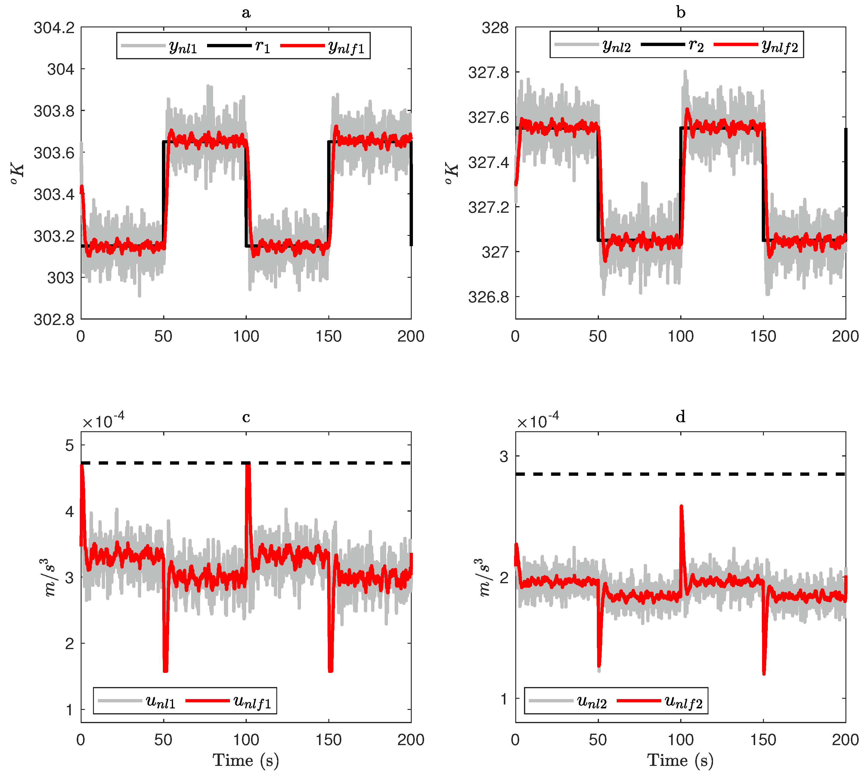
In this case, the results will demonstrate the effect of the filter integrated into the fault estimator and its benefits when filtered measurements are used to compute the control signal, rather than unfiltered measurements. From initial conditions T c o = 303.45 and T h o = 327.25 in the non-linear system, with a measurement noise n s = 5 × 10 4 and a fourth-order Runge–Kutta integration method, Figure 3 shows the simulation results for this case. This test is aimed at showing the MPC control performance by taking into account r = [ r 1 r 2 ] , referring to the desired values for y n l 1 and y n l 2 , respectively. We define the following reference values:
r 1 = 303.15 , 0 t < 50 and 100 t 150 , 303.65 , 50 t < 100 and 150 t 200 , r 2 = 327.55 , 0 t < 50 and 100 t 150 , 327.05 , 50 t < 100 and 150 t 200 .
In Figure 3a,b is possible to see the unfiltered system outputs y n l 1 and y n l 2 associated with T c o and T h o , respectively, reaching the desired values r 1 and r 2 defined in Equation (31). The filtered outputs, labeled as y n l f 1 and y n l f 2 , can be seen in these figures, evolving to the desired reference values with different characteristics over time compared to the unfiltered outputs. Recall that the filter attenuates excessive noise amplitude and thus improves the system performance. Notice that y n l = y l + y 0 = [ y n l 1 y n l 2 ] and y n l f = y l f + y 0 = [ y n l f 1 y n l f 2 ] are defined as the sum of the linear unfiltered output and linear filtered output, respectively, with a constant output value in the operating point. Figure 3c,d present the input flow rate results obtained using the unfiltered and filtered outputs to feed the MPC controller defined in Section 2.2.3. These figures show that using the unfiltered outputs to feed the controller generates control signals ( u n l 1 and u n l 2 ) with higher noise amplitudes compared to the case of using the filtered outputs. In other words, the control signals u n l f 1 and u n l f 2 constructed with the filtered outputs are less noisy than those in the previously mentioned case. Finally, Figure 3c,d illustrate that the constraints imposed by the MPC controller are satisfied (represented by the dotted black line) when tracking the desired reference values. It is worth mentioning that the lower limits of the constraints are not plotted to give a better visualization, since the control signals do not reach these amplitudes. As a final comment, this result shows that the fault-free case within the proposed FTC scheme works properly as expected and designed, giving rise to the following sensor fault case test.

4.2. Faulty Case

The first step to address the faulty case consists of computing the fault estimation observer gain and defining the matrix coefficients Δ e and Δ f r as 1 × 10 2 I and 1 × 10 2 I , respectively, where I is a compatible dimension matrix. Solving the LMI represented by Equation (A6) using Sedumi and Yalmip, we can find the numerical value of the fault estimator observer gain:
K ˜ = 0.449 0.049 0.078 0.548 1.835 0.003 0.002 1.839 3.288 0.007 0.038 3.255 ,
from which, by comparison
K f e = 0.449 0.049 0.078 0.548 1.835 0.003 0.002 1.839 , L f e = 3.288 0.007 0.038 3.255 ,
with a bounding factor ρ = 0.0664 . The observers in charge of generating the fault reconfiguration through the faulty output estimation (included within the observer bank shown in Figure 1, i.e., O 1 and O 2 ) are presented in Table 3. It includes the design parameters for computing their gains by considering Equation (A11).
Table 4 presents general information regarding the fault reconfiguration unit process during the faulty heat exchanger condition. In the fault-free case, the filtered output y l f feeds the MPC controller to compute the control signal, and the alarm is set to 0. In the case of a fault in the output y l f 1 , the alarm equals 1, and the observer O 1 generates the estimated output y ^ l f 1 using the output y l f 2 . After this process, the control signal is generated with y ^ l f 1 and y l f 2 . When a fault occurs in output y l f 2 , the alarm is set to 2 to give a difference compared to the previous case, and the observer O 2 generates the estimated output y ^ l f 2 using y l f 1 to compute the control signal with y l f 1 and y ^ l f 2 .
To evaluate the fault estimator performance, a test is conducted that considers constant and time-varying faults in the non-linear system outputs. The faults f s 1 and f s 2 are defined to have an evolution over time as follows:
f s 1 = 0 , 0 t < 30 , 50 , 30 t < 95 , 0 , 95 t < 280 , 25 sin ( 0.05 t ) + 40 , 280 t < 400 , 0 , 400 t 510 ,
f s 2 = 0 , 0 t < 125 , 30 , 125 t < 180 , t + 175 , 180 t < 240 , 0 , 240 t 440 , 60 , 440 t < 510 ,
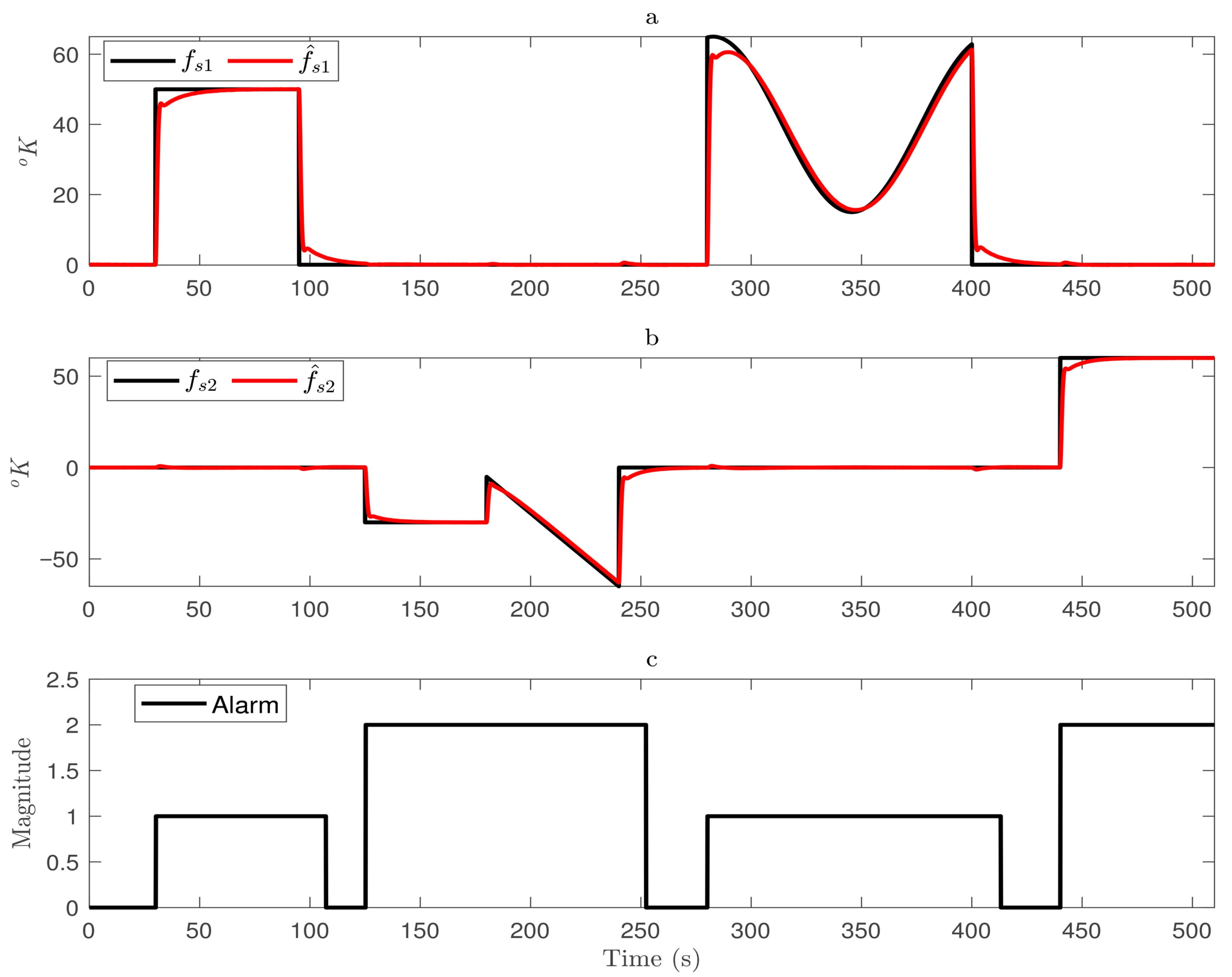
recalling that f s = [ f s 1 f s 2 ] . For this test, a 510 s simulation time has been considered to show the proposed FTC results. With the FTC scheme shown in Figure 1 and the fault estimator observer, the observers for fault reconfiguration, the decision unit, the MPC controller, and the faults defined in Equations (34) and (35), Figure 4 presents the fault estimator performance as a first result.
Figure 4a,b show the fault estimations f ^ s 1 and f ^ s 2 correctly reaching the fault values of f s 1 and f s 2 , respectively. Depending on the faulty output, the corresponding fault alarm indicator is activated (see Figure 4c). Notice that in the case of a fault in y n l 1 , the alarm indicator is set to 1, while in the case of a faulty condition in y n l 2 , the corresponding value is set to 2. Recall that this indicator is activated when the fault exceeds the defined threshold t h = 2 . It is worth mentioning that the threshold must be defined so that the fault estimations, which remain noisy, do not cause false fault alarms, resulting in an unnecessary fault reconfiguration process. It is important to note that the faults occur in terms of temperature to accurately show a sensor’s faulty condition. A positive value in a defined fault is interpreted as a measurement beyond the real value (BIAS), while the loss of effectiveness involves a measurement below the real value. This is an essential issue to consider while analyzing the results presented throughout this paper. As a concluding comment, the results in Figure 4 prove that the fault estimator and the fault alarm indicator perform their tasks correctly, allowing the fault reconfiguration process in the FTC. In turn, Figure 5 and Figure 6 present the simulation results for the system outputs.
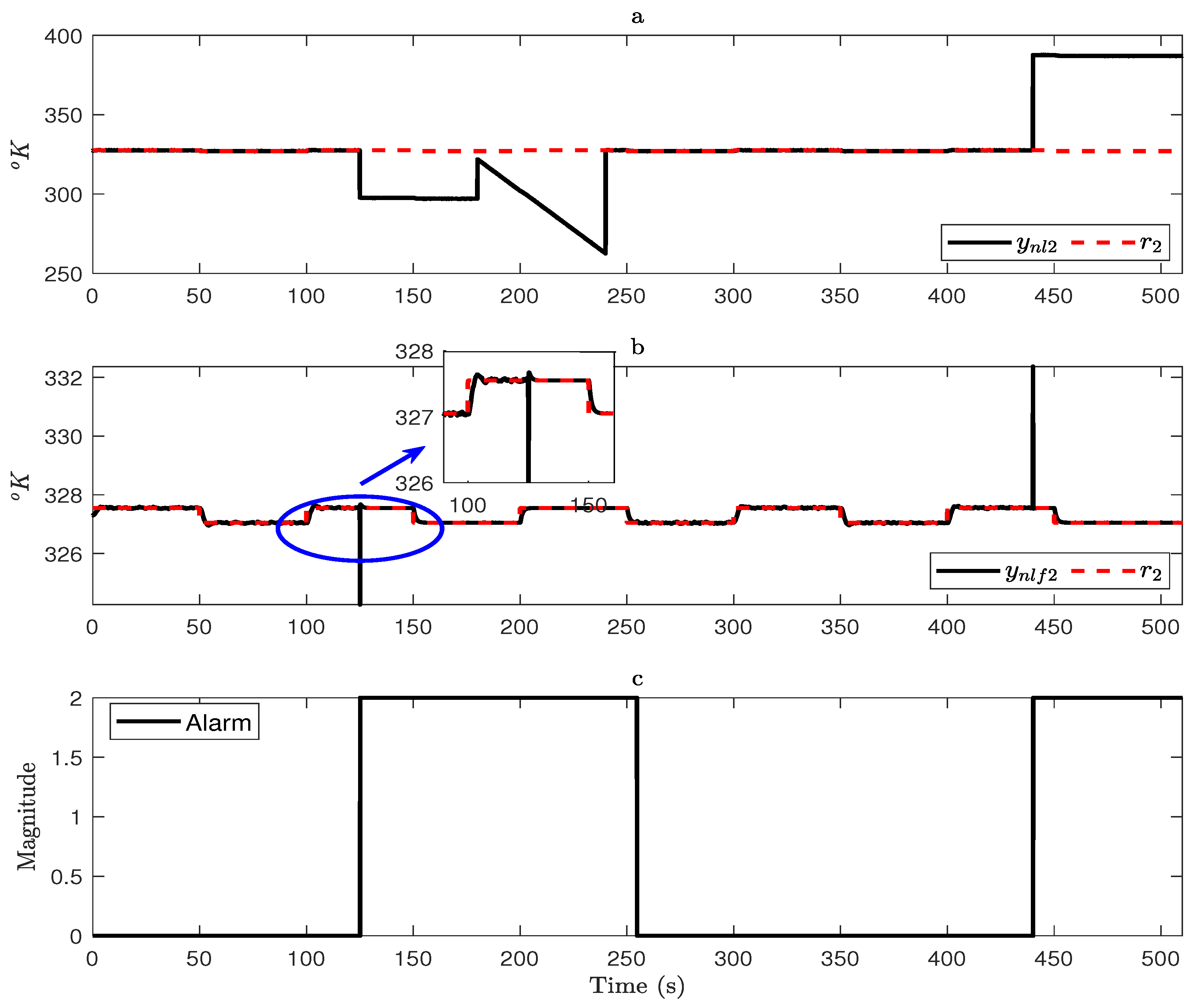
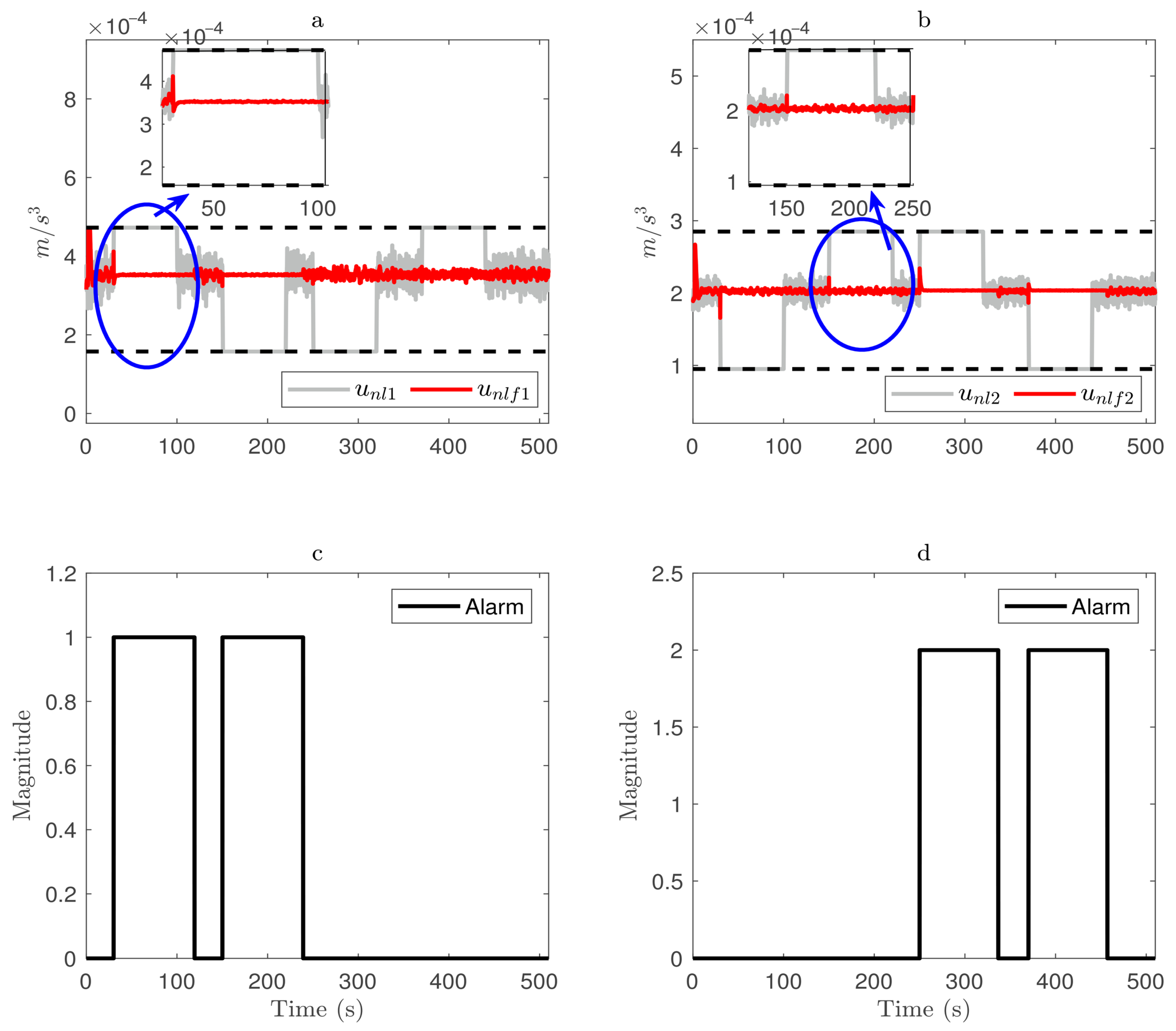
Figure 5a shows the case of a fault in y n l 1 , which is applied at 30 s t < 95 s and 280 s t < 400 s. The condition sets the alarm with magnitude 1 if | f ^ s 1 | > t h , as depicted in Figure 5c. When the alarm is triggered, the fault reconfiguration system constructs the output for control purposes y f c = [ y ^ l f 1 y l f 2 ] , as stated in Table 4. Notice that the observer reconfigures the faulty output, allowing the achievement of the control objectives, as shown in Figure 5b. When the y n l 1 sensor is in a faulty condition and the reconfiguration process is not performed, the system output presents a deviation from the desired value r 1 with a similar evolution over time to f s 1 . In the case of a fault with a time-varying evolution occurring at 280 s t < 400 s (sine wave), in turn, the output presents an offset that follows the fault dynamic (see Figure 5a). A zoom in on the graph at one of the transitions is included at the time of the fault occurrence to give the reader a clearer perspective of the fault reconfiguration process. A similar condition can be seen in the case of a fault in y n l 2 , as shown in Figure 6.
The alarm magnitude is set to 2 when the fault occurs, as shown in Figure 6c. The result related to the FTC performance is presented in Figure 6b. If the reconfiguration process is performed, the system output does not exhibit any offset from the desired reference value r 2 . Notice that an overshoot can be seen when the fault occurs, related to the time between the fault occurrence and the reconfiguration process, or, in other words, the time elapsed from the fault occurrence to the condition of | f ^ s 2 | > t h . On the other hand, suppose the reconfiguration process is not performed, as shown in Figure 6a. In this case, the output has an offset, causing poor performance of the MPC controller and thus a lack of achievement of control objectives.
Finally, Figure 7 depicts the control signals in the faulty case. In Figure 7, the light grey graphs represent the system output when fault reconfiguration is not performed, while the rest of the graphs refer to the operation of the proposed FTC system. Figure 7a presents the results for fault occurrence in y n l 1 , focusing specifically on 30 s t < 95 s and 280 s t < 400 s. Notice that the control law u n l 1 generated when fault reconfiguration is not performed shows saturation in its magnitude due to the constraints set in the MPC design. Otherwise, if fault reconfiguration is performed, the control signal evolves as in the fault-free case with a transient during the reconfiguration process. Figure 7b shows the corresponding result for the fault occurrence in y n l 2 . The control signal, u n l f 2 , provides the correct tracking reference despite the occurrence of the fault due to the fault reconfiguration process. However, if the fault reconfiguration process is not performed, the control input u n l 2 also presents saturation due to the constraints set in the MPC controller design. Finally, the corresponding alarms are presented in Figure 7c,d.
As a second test, the following addresses the faults in the worst case that the proposed FTC scheme can deal with. For this, constant references r 1 = 302.9 and r 2 = 327.8 in t ≥ 2s ( r 1 = x n l 1 and r 2 = x n l 2 0 t 2 ) were considered by maintaining the observer for fault estimation, the observer for fault reconfiguration, and the sensor fault reconfiguration unit as in the previous test. The applied faults were defined as follows:
f s 1 = 0 , 0 t < 30 , 100 , 30 t < 100 , 0 , 100 t < 150 , 100 , 150 t < 220 , 0 , 220 t 510 ,
f s 2 = 0 , 0 t < 250 , 100 , 250 t < 320 , 0 , 320 t < 370 , 100 , 370 t 440 , 0 , 440 t < 510 .
It is important to note that the fault magnitudes considered for this test represent approximately 30% of BIAS or loss of effectiveness concerning the operating point x 0 n l involved in the linearization process. Figure 8 shows the performance of the fault estimator for this test. From Figure 8, the correct fault estimation is observed, showing in Figure 8a,b the applied faults and their estimations. Figure 8c, in turn, depicts the corresponding fault alarm. Let us point out that although the fault estimator is designed for the linearized system, it can estimate the occurred fault correctly.
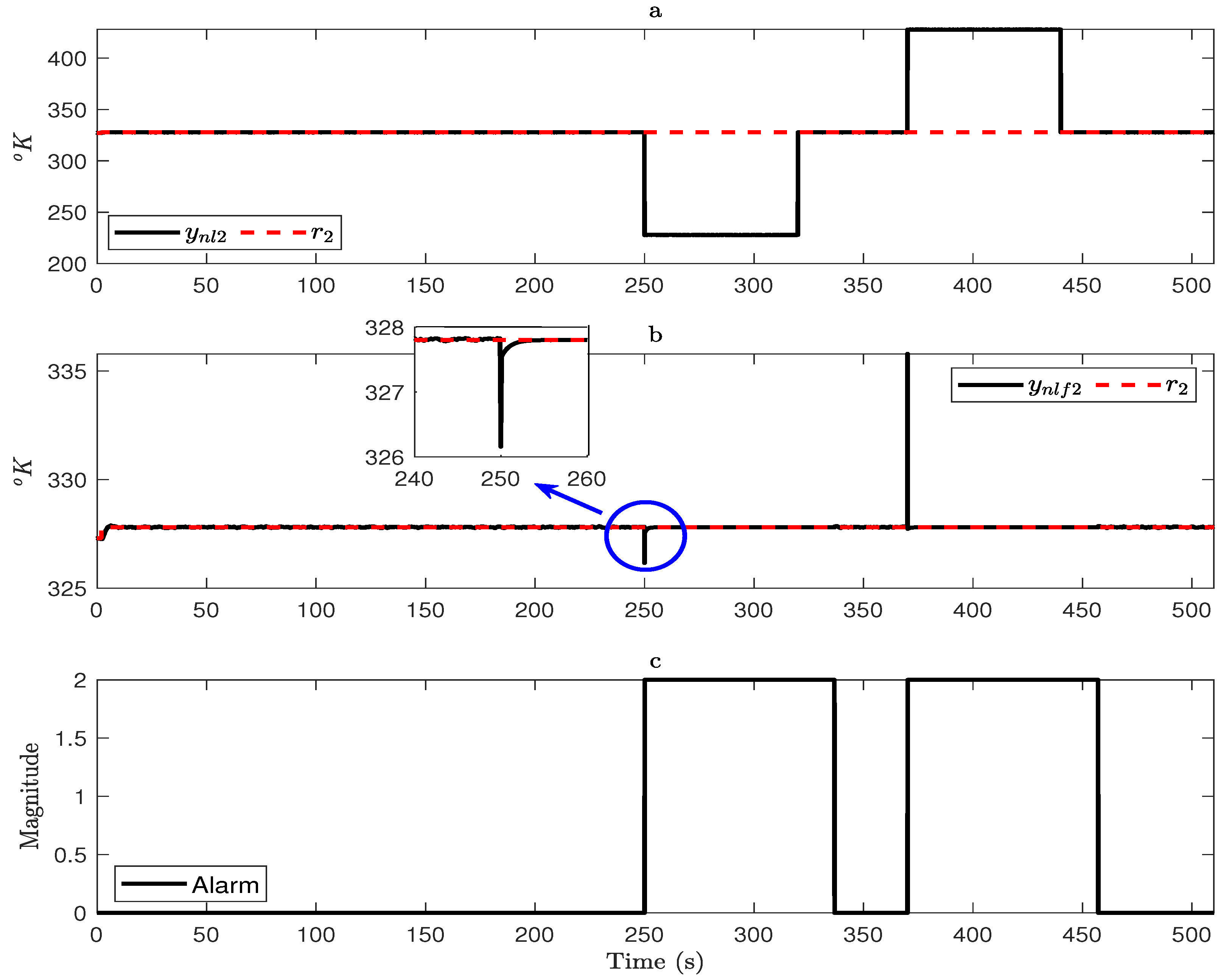
As for the system outputs, in turn, Figure 9 and Figure 10 present their corresponding results. Recalling that in this test the faults are considered in a steady-state condition for the system with constant references, Figure 9a shows the output y n l . Its magnitude follows the applied fault, increasing or decreasing its value according to the faulty condition defined in Equation (36). In turn, Figure 9b depicts the FTC operation, giving rise to the reconfigured output y n l f 1 . From the zoom presented in the figure, the control objective achievement can be seen due to the condition y n l f 1 = r 1 t 2 s. The FTC works properly despite the fault magnitude. The alarm generated in this case is depicted in Figure 9c, changing its value depending on the faulty sensor. Finally, Figure 10 shows the result of addressing the remaining output. A similar interpretation must be considered for analyzing Figure 10. The faulty output y n l 2 , the corresponding reconstruction y n l f 2 , and the alarm can be seen in Figure 10a, Figure 10b and Figure 10c, respectively.
Regarding the control signal involved in the present faulty case, Figure 11 shows the input flow rate results obtained using the unfiltered and filtered outputs to feed the MPC controller defined in Section 2.2.3. Figure 11a,b depict the control signals u n l 1 and u n l 2 , presenting a saturation in faulty conditions as a consequence of the MPC design. The control signals u n l f 1 and u n l f 2 , constructed with the filtered outputs, are less noisy with respect to u n l 1 and u n l 2 and can achieve the control objectives despite the fault occurrence. Finally, from the results presented within the faulty case condition in the non-linear system, a correct operation of the proposed FTC system can be defined.

5. Discussion

The present results show that the FTC proposed in this paper operates properly, achieving the control objectives for the case study. However, some aspects are worth discussing to address limitations and enhance the contribution and future works related to the presented proposal.
  • Regarding the measured noise in the proposed FTC scheme, it is important to note that the FTC considers its representation in the system dynamics analytically, giving rise to the FTC element design. The proposed FTC scheme includes these elements to deal with the measurement noise, defining the main contribution of the present paper.
  • In addressing the proposed FTC scheme for the control law, it is relevant to note that the MPC controller cannot attenuate the sensor fault effect, which makes the proposed FTC scheme suitable. Besides this condition, let us point out that its design, from the results shown throughout this paper, presents the achievement of the boundary conditions correctly, included within its analytical design. In this sense, note that the system outputs exhibit a saturation evolution over time in the faulty case, from which the correct controller performance can be defined. As a concluding comment, let us mention that the designer can choose the design parameters to reach specific transient responses and boundary conditions, depending on the addressed dynamical system.
  • Regarding the observer for fault estimation and observers for fault reconfiguration, it is essential to point out that they contribute to mitigating/reducing the effect of the measurement noise on their corresponding estimations. These elements include specific terms in charge of having this effect on their results, which in the present paper refers to the control law computation aiming at achieving the control objectives with a noise reduction within the closed-loop system dynamics.
  • Let us focus on the faulty case. It is important to note that under faulty sensor operation, physically, the corresponding element will continue providing a measurement that does not accurately reflect the real variable value. However, the output of the system will remain at the desired values due to the FTC system operation as a consequence of the fault reconfiguration process. The real value for the output will be provided by the observer (virtual sensor), which does not consider the faulty output for its estimation.
  • On the other hand, an important issue is related to the threshold t h involved in triggering the fault alarm. Note that its value depends on how fast the fault must be detected and isolated. In the present paper, this condition refers to the t h selection considering the remaining noise presented in the fault estimations. A threshold defined close to the remaining noise in the fault estimation could lead to an unnecessary reconfiguration process and thus to an unnecessary switching behavior between the observers for fault reconfiguration. As a result, its selection depends on the measurement noise presented in the system, from which the fault occurrence is defined.
  • Following with the threshold t h and aiming at explicitly mentioning its importance, in the present paper, the selected value is defined in such a way that the result of the proposed method can be generated. The authors consider that further analysis is necessary in real scenarios to ensure the optimal value, possibly an optimization process from data provided by the real system instrumentation. This condition will generate more accurate results when handling real systems.
  • It is worth mentioning the motivation behind this paper in contrast with existing methods handling the measurement noise within dynamical systems. Although several works have been reported regarding sensor noise, as an example, those presented in [39,40], the results presented in this paper consider functional observers to provide fault recovery in the case of faulty conditions in the system outputs. The authors mention that future research directions could utilize more complex schemes regarding the elements in charge of providing fault and state reconstruction, dealing with measurement noise, in the context of FCT systems.
  • In addressing the second result shown in the corresponding section, it is essential to mention that faults with values ± 100 are considered the worst case that the proposed FTC scheme can deal with. In the simulation, the authors applied fault magnitudes beyond this value, making the system unsolvable. Notice that despite this fact, the proposed FTC deals with BIAS or loss of effectiveness in the sensor around 30% regarding the operating point considered in the linearization process for FTC design. Along with this consideration, the observer for fault estimation and the MPC controller can provide information for the operation of the reconfiguration unit, giving accurate results. Note that the MPC controller bounds the control signals. As long as the solution to the optimization problem is feasible, the system maintains stability by having the inputs bounded under defined fault conditions. These issues can define that linear approaches can be considered for dealing with non-linear systems.
  • Regarding the heat exchanger’s non-linear dynamics, the condition related to Δ T is worth mentioning. Notice that this condition involves the quotient between the difference of temperatures and a natural logarithm. It is well known that this function is not defined in 0, giving rise to an undefined Δ T and, consequently, unsolvable dynamics. This consideration is a limitation and a challenging problem when dealing with the heat exchanger approximated by the model addressed in this paper.
  • As a concluding comment, the present study allows us to define extensions of FTC towards linear systems by considering possible actuator faults or simultaneous sensor and actuator faults in a dynamical system affected by measurement noise. Also, different controllers can be implemented within this FTC scheme to ensure defined control objectives, allowing, as a result, the proposed FTC control system extension. These issues are future research directions regarding FTC in dynamical systems with outputs measured with noise.

6. Conclusions

This paper presents and applies an FTC system design to a counter-flow heat exchanger. The proposed FTC design considers measurement noise, which gives closer results to real-time systems. Its design refers analytical procedures to deal with the noise presented at the system outputs, including elements coping with this condition to compute a control law with less measurement noise concerning the real outputs. The results demonstrate that the proposed FTC operates effectively in a faulty case when sensor faults with both constant and time-varying dynamical evolution occur. The FTC includes an MPC controller to establish control objectives over the system outputs, achieving fault tolerance for sensor faults.

Author Contributions

Writing—original draft: J.A.B.-M. Methodology and formal analysis: J.A.B.-M. and F.D.J.S.-V. Conceptualization and investigation: G.O.-T. and J.Y.R.-M. Writing—review and editing: C.A.T.-C. and M.R.-M. Software: A.F.P.-V. All authors have read and agreed to the published version of the manuscript.

Funding

This research received no external funding.

Conflicts of Interest

The authors declare no conflicts of interest.

Appendix A

Appendix A.1. Fault Estimator Design

From Equation (9), considering the estimation error dynamics as in Equation (6) yields the following:
e P [ A e e + D e f r ] + [ A e e + D e f r ] P e + . . . . . . e Δ e e σ 2 f r Δ f r f r 0 , e P A e e + e P D e f r + e A e P e + f r D e P e + . . . . . . e Δ e e σ 2 f r Δ f r f r 0 .
Equation (A1), as a consequence, can be expressed in matrix form by gathering e and f r as follows:
e f r P A e + A e P + Δ e P D e D e P σ 2 Δ f r e f r 0 ,
from which the state and fault estimation error convergence is ensured if
P A e + A e P + Δ e P D e D e P σ 2 Δ f r 0 .
As such, the accomplishment of Equation (A3) is required to reach the objectives of the fault estimation observer. To compute the observer gain, let us focus on A e from Equation (7), with an equivalent representation as follows:
A e = A a C f s a 0 0 K f e L f e C a 0 = A ˜ e K ˜ C ˜ a ,
giving rise to its substitution into Equation (A3):
P ( A ˜ e K ˜ C ˜ a ) + ( A ˜ e K ˜ C ˜ a ) P + Δ e P D e D e P σ 2 Δ f r 0 .
Finally, to eliminate the bilinearity conditions P K ˜ and σ 2 , by considering K ¯ = P K ˜ and σ 2 = χ , the linear matrix inequality (LMI)
P A ˜ e K ¯ C ˜ a + A ˜ e P C ˜ a K ¯ + Δ e P D e D e P χ Δ f r 0 ,
concludes the observer design. The achievement of the LMI (A6) will ensure that both e e and e f will converge to zero as t with the observer gains K ˜ = P 1 K ¯ and a bounding factor σ = χ , ending with the proof of Theorem 1.

Appendix A.2. Observer Design for Fault Reconfiguration

From Equation (14), by considering Equation (13)
e a c P a c [ A a c e a c D a c n s ] + [ A a c e a c D a c n s ] P a c e a c + . . . . . . e a c Δ a c e a c ρ 2 n s Δ n s n s 0 , e a c P a c A a c e a c e a c P a c D a c n s + e a c A a c P a c e a c . . . . . . n s D a c P a c e a c + e a c Δ a c e a c ρ 2 n s Δ n s n s 0 .
From here, a straightforward calculation can be performed by considering e a c and n s in matrix form, as shown in the procedure outlined in Equations (A2) and (A3):
P a c A a c + A a c P a c + Δ a c P a c D a c D a c P a c ρ 2 Δ n s 0 ,
giving rise to the state error convergence if satisfied. In turn, notice that by considering L ˜ a c = P a c L a c
P a c A a c = P a c ( A L a c C a c ) , = P a c A L ˜ a c C a c ,
and
P a c D a c = P a c L a c C a c , = L ˜ a c C a c .
Finally, by subsituting Equations (A9) and (A10) into Equation (A8), we get
Ξ + Ξ + Δ a c L ˜ a c C a c C a c L ˜ a c χ a c Δ n s 0 ,
with Ξ = P a c A a c L ˜ a c C a c , χ a c = ρ 2 and the observer gain computed by L a c = P a c 1 L ˜ a c . The proof of Theorem 2, as a consequence, is concluded.

References

  1. Abbaspour, A.; Mokhtari, S.; Sargolzaei, A.; Yen, K.K. A Survey on Active Fault-Tolerant Control Systems. Electronics 2020, 9, 1513. [Google Scholar] [CrossRef]
  2. Brizuela-Mendoza, J.A.; Sorcia-Vázquez, F.D.J.; Rumbo-Morales, J.Y.; Lozoya-Ponce, R.E.; Rodríguez-Cerda, J.C. Active fault tolerant control based on eigenstructure assignment applied to a 3-DOF helicopter. Asian J. Control 2021, 23, 673–684. [Google Scholar] [CrossRef]
  3. Ortiz-Torres, G.; Rumbo-Morales, J.; Sorcia-Vázquez, F.; Pérez-Vidal, A.; Cruz-Rojas, A.; Brizuela-Mendoza, J.; Oceguera-Contreras, E. Concentration estimation and fault tolerant control in a CSTR modelled as a quasi linear parameter varying system. Rev. Mex. Ing. Química 2021, 20, 51–66. [Google Scholar] [CrossRef]
  4. Zhu, F.; Fu, Y.; Dinh, T.N. Asymptotic convergence unknown input observer design via interval observer. Automatica 2023, 147, 110744. [Google Scholar] [CrossRef]
  5. Zhu, F.; Li, M. Distributed Interval Observer and Distributed Unknown Input Observer Designs. IEEE Trans. Autom. Control 2024, 69, 8868–8875. [Google Scholar] [CrossRef]
  6. Hanif, O.; Deshpande, N.G.; Chatterjee, M. Identification and Control of a Heat Exchanger. In Proceedings of the 2021 International Symposium of Asian Control Association on Intelligent Robotics and Industrial Automation (IRIA), Goa, India, 20–22 September 2021; pp. 259–264. [Google Scholar]
  7. Jin, Y.; Sun, L.; Hua, Q.; Chen, S. Experimental Research on Heat Exchanger Control Based on Hybrid Time and Frequency Domain Identification. Sustainability 2018, 10, 2667. [Google Scholar] [CrossRef]
  8. Miao, W.; Xu, B. Application of Feedforward Cascade Compound Control Based on Improved Predictive Functional Control in Heat Exchanger Outlet Temperature System. Appl. Sci. 2023, 13, 7132. [Google Scholar] [CrossRef]
  9. Al-Dhaifallah, M. Fuzzy fractional-order PID control for heat exchanger. Alex. Eng. J. 2023, 63, 11–16. [Google Scholar] [CrossRef]
  10. Fürst, Y.; Brandt, S.; Kriegel, M. Introducing a new nonlinear approach to model heat exchangers designed for control engineering applications. Eur. J. Control 2024, 79, 101072. [Google Scholar] [CrossRef]
  11. Amin, A.A.; Hasan, K.M. A review of Fault Tolerant Control Systems: Advancements and applications. Measurement 2019, 143, 58–68. [Google Scholar] [CrossRef]
  12. Ortiz-Torres, G.; Valdez-Resendiz, J.E.; Torres-Cantero, C.A.; Rumbo-Morales, J.Y.; Ramos-Martinez, M.B.; Valdez-Martinez, J.S. Actuator and Sensor Fault Detection and Isolation System Applied to a Distillation Column. IEEE Access 2023, 11, 48548–48558. [Google Scholar] [CrossRef]
  13. Ortiz Torres, G.; Rumbo Morales, J.Y.; Ramos Martinez, M.; Valdez-Martínez, J.S.; Calixto-Rodriguez, M.; Sarmiento-Bustos, E.; Torres Cantero, C.A.; Buenabad-Arias, H.M. Active Fault-Tolerant Control Applied to a Pressure Swing Adsorption Process for the Production of Bio-Hydrogen. Mathematics 2023, 11, 1129. [Google Scholar] [CrossRef]
  14. Escobar-Jimenez, R.F.; Carbot-Rojas, D.A.; Gómez-Aguilar, J.F.; Alvarado-Martínez, V.M.; Téllez-Anguiano, A.C.; Hernandez-Perez, J.A. Actuator Fault Tolerant Control Based on a MIMO-MPC: Application in a Double-Pipe Heat Exchanger. Chem. Eng. Commun. 2017, 204, 86–96. [Google Scholar] [CrossRef]
  15. Carbot-Rojas, D.; Escobar, R.; Gómez-Aguilar, J.; López-López, G.; Olivares-Peregrino, V. Experimental validation of an actuator fault tolerant control system using virtual sensor: Application in a double pipe heat exchanger. Chem. Eng. Res. Des. 2015, 104, 400–408. [Google Scholar] [CrossRef]
  16. Escobar, R.; Astorga-Zaragoza, C.; Téllez-Anguiano, A.; Juárez-Romero, D.; Hernández, J.; Guerrero-Ramírez, G. Sensor fault detection and isolation via high-gain observers: Application to a double-pipe heat exchanger. ISA Trans. 2011, 50, 480–486. [Google Scholar] [CrossRef] [PubMed]
  17. Alegría-Zamudio, M.; Escobar-Jiménez, R.; Gómez-Aguilar, J. Fault tolerant system based on non-integers order observers: Application in a heat exchanger. ISA Trans. 2018, 80, 286–296. [Google Scholar] [CrossRef] [PubMed]
  18. Han, X.; Rammal, R.; Li, Z.; Cabassud, M.; Dahhou, B. Interval Observer-Based Active Fault Tolerant Control for an Intensified Heat Exchanger/Reactor. In Proceedings of the 2021 9th International Conference on Systems and Control (ICSC), Caen, France, 24–26 November 2021; pp. 133–138. [Google Scholar]
  19. Wang, J.; Sun, J.; Ge, W.; Zhang, F.; Gao, R.X. Virtual Sensing for Online Fault Diagnosis of Heat Exchangers. IEEE Trans. Instrum. Meas. 2022, 71, 1–8. [Google Scholar] [CrossRef]
  20. Han, X.; Rammal, R.; He, M.; Li, Z.; Cabassud, M.; Dahhou, B. Dynamic and sensor fault tolerant control for an intensified heat-exchanger/reactor. Eur. J. Control 2023, 69, 100736. [Google Scholar] [CrossRef]
  21. Morato, M.M.; Felix, M.S. Data Science and Model Predictive Control: A survey of recent advances on data-driven MPC algorithms. J. Process Control 2024, 144, 103327. [Google Scholar] [CrossRef]
  22. García, C.E.; Prett, D.M.; Morari, M. Model predictive control: Theory and practice—A survey. Automatica 1989, 25, 335–348. [Google Scholar] [CrossRef]
  23. Siza, J.; Llanos, J.; Velasco, P.; Moya, A.P.; Sumba, H. Model Predictive Control (MPC) of a Countercurrent Flow Plate Heat Exchanger in a Virtual Environment. Sensors 2024, 24, 4511. [Google Scholar] [CrossRef] [PubMed]
  24. Dyrska, R.; Horváthová, M.; Bakaráč, P.; Mönnigmann, M.; Oravec, J. Heat exchanger control using model predictive control with constraint removal. Appl. Therm. Eng. 2023, 227, 120366. [Google Scholar] [CrossRef]
  25. Liu, R.; Li, Y. A review of fault tolerant control based on Model Predictive Control. In Proceedings of the 2022 37th Youth Academic Annual Conference of Chinese Association of Automation (YAC), Beijing, China, 19–20 November 2022; pp. 818–823. [Google Scholar]
  26. Bavili, R.E.; Mohammadzadeh, A.; Tavoosi, J.; Mobayen, S.; Assawinchaichote, W.; Asad, J.H.; Mosavi, A.H. A New Active Fault Tolerant Control System: Predictive Online Fault Estimation. IEEE Access 2021, 9, 118461–118471. [Google Scholar] [CrossRef]
  27. Feng, X.; Patton, R. Active Fault Tolerant Control of a Wind Turbine via Fuzzy MPC and Moving Horizon Estimation. In Proceedings of the 19th IFAC World Congress, Cape Town, South Africa, 24–29 August 2014; Volume 47, pp. 3633–3638. [Google Scholar]
  28. Ranjan, R.; Kravaris, C. Model-predictive fault-tolerant control of safety-critical processes based on dynamic safe set. J. Process Control 2024, 144, 103329. [Google Scholar] [CrossRef]
  29. Xiao, G.; Liu, F. Distributed fault-tolerant model predictive control for intermittent fault: A cooperative way. ISA Trans. 2019, 89, 113–121. [Google Scholar] [CrossRef]
  30. Wang, S.; Li, H.; Li, H.; Shi, H.; Sun, Q.; Li, P. Dynamic output feedback robust MPC hybrid fault-tolerant control for discrete uncertain systems: A switching control strategy. Int. J. Control 2025, 98, 1518–1531. [Google Scholar] [CrossRef]
  31. He, M.; Li, Z.; Han, X.; Dahhou, B.; Cabassud, M. Study on Fault Tolerant Control of an Intensified Heat-Exchanger/Reactor Using Two-Layer Multiple Model Structure, Proceedings of the 15th European Workshop on Advanced Control and Diagnosis (ACD 2019), Bologna, Italy, 21–22 November 2019; Zattoni, E., Simani, S., Conte, G., Eds.; Springer International Publishing: Cham, Switzerland, 2022; pp. 295–312. [Google Scholar]
  32. Zhang, B.; Sun, X.; Liu, S.; Deng, X. Distributed fault tolerant model predictive control for multi-unmanned aerial vehicle system. Asian J. Control 2022, 24, 1273–1292. [Google Scholar] [CrossRef]
  33. Oh, S.; Song, T.; Kim, M.; Oh, K.S. Adaptive Model Predictive Fault-Tolerant Control for Four-Wheel Independent Steering Vehicles with Sensitivity Estimation. Int. J. Automot. Technol. 2023, 24, 829–850. [Google Scholar] [CrossRef]
  34. Bakhtiaridoust, M.; Yadegar, M.; Jahangiri, F. Koopman fault-tolerant model predictive control. IET Control Theory Appl. 2024, 18, 939–950. [Google Scholar] [CrossRef]
  35. Khedher, A.; Benothman, K.; Maquin, D.; Benrejeb, M. State and sensor faults estimation via a proportional integral observer. In Proceedings of the 2009 6th International Multi-Conference on Systems, Signals and Devices, Djerba, Tunisia, 23–26 March 2009; pp. 1–6. [Google Scholar]
  36. Rossiter, J.A. Model-Based Predictive Control: A Practical Approach; CRC Press: Boca Raton, FL, USA, 2003. [Google Scholar]
  37. Camacho, E.F.; Bordons, C. Model Predictive Control; Springer: Berlin/Heidelberg, Germany, 2002. [Google Scholar]
  38. Astorga-Zaragoza, C.M.; Zavala-Río, A.; Alvarado, V.; Méndez, R.M.; Reyes-Reyes, J. Performance monitoring of heat exchangers via adaptive observers. Measurement 2007, 40, 392–405. [Google Scholar] [CrossRef]
  39. Zhang, S.; Qi, X.; Yang, S. An Extended State Observer with Adjustable Bandwidth for Measurement Noise. J. Syst. Eng. Electron. 2024, 35, 233–241. [Google Scholar] [CrossRef]
  40. Battilotti, S. Robust observer design under measurement noise with gain adaptation and saturated estimates. Automatica 2017, 81, 75–86. [Google Scholar] [CrossRef]
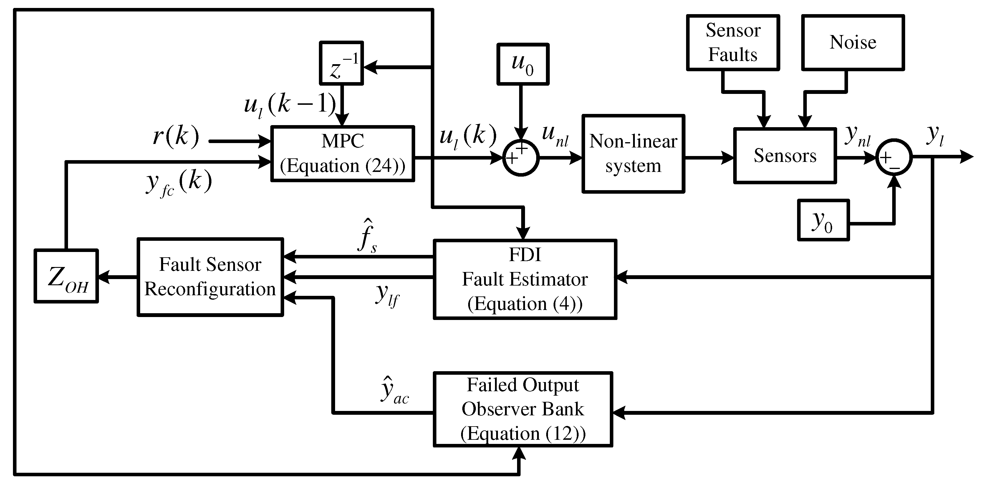
Figure 1. Fault-tolerant control system.
Automation 06 00048 g001
Figure 2. Heat exchanger variable schematic.
Automation 06 00048 g002
Figure 3. Fault-free case simulation results. (a) System output y n l 1 , y n l f 1 , and reference r 1 . (b) System output y n l 2 , y n l f 2 , and reference r 2 . (c) Control law u n l 1 and u n l f 1 . (d) Control law u n l 2 and u n l f 2 .
Automation 06 00048 g003
Figure 4. First test fault estimation results. (a) Fault f s 1 and its estimation. (b) Fault f s 2 and its estimation. (c) Alarm.
Automation 06 00048 g004
Figure 5. First test faulty case: output T c o . (a) Output y n l 1 and reference r 1 . (b) Output y n l f 1 and reference r 1 . (c) Alarm.
Automation 06 00048 g005
Figure 6. First test faulty case: output T h o . (a) Output y n l 2 and reference r 2 . (b) Output y n l f 2 and reference r 2 . (c) Alarm.
Automation 06 00048 g006
Figure 7. First test faulty case: control signals. (a) Control law u n l 1 and u n l f 1 . (b) Control law u n l 2 and u n l f 2 . (c) Alarm in a fault in sensor T c o . (d) Alarm in a fault in sensor T h o .
Automation 06 00048 g007
Figure 8. Second test fault estimation results. (a) Fault f s 1 and its estimation. (b) Fault f s 2 and its estimation. (c) Alarm.
Automation 06 00048 g008
Figure 9. Second test faulty case: output T c o . (a) Output y n l 1 and reference r 1 . (b) Output y n l f 1 and reference r 1 . (c) Alarm.
Automation 06 00048 g009
Figure 10. Second test faulty case: output T h o . (a) Output y n l 2 and reference r 2 . (b) Output y n l f 2 and reference r 2 . (c) Alarm.
Automation 06 00048 g010
Figure 11. Second test faulty case: control signals. (a) Control law u n l 1 and u n l f 1 . (b) Control law u n l 2 and u n l f 2 . (c) Alarm in a fault in sensor T c o . (d) Alarm in a fault in sensor T h o .
Automation 06 00048 g011
Table 1. Heat exchanger parameter description.
ParameterDescriptionValueUnit
T c i Inlet temperature on the cold side298K
T h i Inlet temperature on the hot side338K
UHeat transfer coefficient160J/(m2K s)
AHeat transfer surface area 0.633 m2
c p c Specific heat on the cold side1910J/(Kg K)
c p h Specific heat on the hot side1519J/(Kg K)
ρ c Density of the cold side1000kg/m3
ρ h Density of the hot side1000kg/m3
V c Volume on the cold side 6.05 × 10 3 m3
V h Volume on the hot side 3.2 × 10 3 m3
Table 2. MPC controller tuning parameters.
SymbolParameterValue
n y Prediction Horizon50
n c Control Horizon15
α Error Tracking Weight 0.9 I q × q
λ Input Increment Weight 10 I p × p
Table 3. Fault reconfiguration observer parameters.
ObserverParameter DesignObserver Gain χ ac
O 1 Δ e a c = 1 × 10 1 I
Δ n s = 1 × 10 2 I
L 1 = 0.1057 1.2894 χ a c 1 = 0.0965
O 2 Δ e a c = 1 × 10 1 I
Δ n s = 1 × 10 2 I
L 2 = 1.2106 0.0465 χ a c 2 = 0.0957
Table 4. Operation of the sensor fault reconfiguration unit.
AlarmMeaningObserverTo Compute y fc for Control
0Fault-free--= y l f
1Fault in y l f 1 O 1 with y l f 2 y ^ l f 1 = [ y ^ l f 1 y l f 2 ]
2Fault in y l f 2 O 2 with y l f 1 y ^ l f 2 = [ y l f 1 y ^ l f 2 ]
Disclaimer/Publisher’s Note: The statements, opinions and data contained in all publications are solely those of the individual author(s) and contributor(s) and not of MDPI and/or the editor(s). MDPI and/or the editor(s) disclaim responsibility for any injury to people or property resulting from any ideas, methods, instructions or products referred to in the content.