Article

Mask Inflation Encoder and Quasi-Dynamic Thresholding Outlier Detection in Cellular Networks

1
Faculty of Telecommunications, Technical University of Sofia, Bul. Kl. Ohridski 8, 1000 Sofia, Bulgaria
2
Intelligent Communication Infrastructure Laboratory, Sofia Tech Park, 1784 Sofia, Bulgaria
*
Author to whom correspondence should be addressed.
Telecom 2025, 6(4), 84; https://doi.org/10.3390/telecom6040084
Submission received: 15 August 2025 / Revised: 11 October 2025 / Accepted: 24 October 2025 / Published: 4 November 2025

Abstract

Mobile networks have advanced significantly, providing high-throughput voice, video, and integrated data access to support connectivity through various services to facilitate high user density. This traffic growth has also increased the complexity of outlier detection (OD) for fraudster identification, fault detection, and protecting network infrastructure and its users against cybersecurity threats. Autoencoder (AE) models are widely used for outlier detection (OD) on unlabeled and temporal data; however, they rely on fixed anomaly thresholds and anomaly-free training data, which are both difficult to obtain in practice. This paper introduces statistical masking in the encoder to enhance learning from nearly normal data by flagging potential outliers. It also proposes a quasidynamic threshold mechanism that adapts to reconstruction errors, improving detection by up to 3% median area under the receiver operating characteristic (AUROC) compared to the standard 95% threshold used in base AE models. Extensive experiments on the Milan Human Telecommunications Interaction (HTA) dataset validate the performance of the proposed methods. Combined, these two techniques yield a 31% improvement in AUROC and a 34% lower computational complexity when compared to baseline AE, long short-term memory AE (LSTM-AE), and seasonal auto-regressive integrated moving average (SARIMA), enabling efficient OD in modern cellular networks.

1. Introduction

The three major components of mobile networks are user equipment (UE), allowing the users to connect to the network; the radio access network (RAN), providing wireless connection to UE; and the core network (CN), which facilitates connectivity and operative functions such as authentication, call routing, billing, and more. To connect millions of customers, networks require densely deployed base stations and, occasionally, multioperator core networks. Maintaining network performance and providing communication services to all customers while preventing fraud and network abuse requires intensive monitoring of the entire network and service usage, together with proactive adjustment of system parameters and identification of fraudulent devices. To achieve this, device and usage logs are systematically collected and analyzed via usage pattern recognition to detect anomalies for fault detection and mitigation of security threats. These use-cases are even more valid today with the roll-out of 5G and beyond networks [1], enabling the dense deployment of various types of UEs with different throughput requirements. A subset of the data collected in mobile communication network operations, termed call-detail records (CDR), is related to human telecommunication activity (HTA). These logs are collected by the UEs, RAN, and coverage area (groups of RANs)—collectively called a grid—and are continuously streamed and made usable for analysis. Regardless of the point of collection and level of aggregation, analyzing such data, making intelligent decisions, and triggering appropriate actions requires the development of anomaly-detection techniques adapted for a particular use case, allowing the system to operate with a greater degree of autonomy [2,3]. OD has also been explored in Open-RAN (O-RAN), which has been established as a novel paradigm for cellular network implementation, as it provides open interfaces and protocols that can be realized on non-proprietary hardware [4]. This architecture includes the near-real-time RAN Intelligent Controller (RIC), which implements adaptive functions for resource allocation, energy management, security, and traffic control, including OD. Additionally, the development of unsupervised anomaly-detection techniques based on unlabeled data to support these use-cases is increasingly relevant in modern cellular networks. Accurate anomaly detection in such data requires first scoring observation normality using a scale, then separating normal from abnormal data via an objective threshold; in many cases, this is performed without empirical knowledge of any usage pattern. For anomaly detection in unlabeled streaming data [5], it is recommended to use statistical methods such as the median absolute deviation (MAD) or Chebyshev’s inequality, which are robust when handling skewed data with outliers but are limited to univariate distributions; the Z-score method under the assumption of data normality; or deep learning (DL) models such as autoencoders (AEs), neural networks (NNs), and generative adversarial networks (GANs) designed to use unlabeled data. These models achieve superior detection accuracy [2] but impart a higher computational cost.
This paper proposes an approach to objectively skew AE-based model training towards normality by providing some statistical context to the data during the learning phase and proposes an objective threshold selection mechanism to improve accuracy in separating data between normal and abnormal observations. The contributions of this paper are as follows:
  • An encoder mask inflation mechanism for an AE model, called Informer, which is used to bias the encoder’s attention towards likely abnormal observations by generating an early anomaly score using statistical normality. This mechanism is combined with quasi-dynamic thresholding based on well-established statistical techniques (Z-score, Chebyshev’s inequality, and MAD) for outlier detection (OD) in mobile networks. It is based on the assumption that anomalies produce higher reconstruction errors and there are fewer anomalies than normal observations, resulting in a right-skewed error distribution.
  • The proposed model uses the Z-score, Chebyshev, and MAD methods to define the thresholds for outliers, and introduces a voting scheme that flags anomalies based on agreement between the best combinations of approaches for encoder-masking and thresholding. This novel solution is applied to the Milano HTA dataset, achieving 31% improvement of the area under the receiver operating characteristic (AUROC), with lower memory requirements and similar computational complexity, compared to relevant OD methods.
Figure 1 below summarizes the proposed method’s operation in processing the input data samples x by the AE model. It incorporates the statistical masking functions Z ( x ) , the objective quasi-dynamic thresholding functions T ( x ) , and the voting-based strategy that determines outliers through majority consensus.
The rest of this article is organized as follows. Section 2 reviews the state-of-the-art in OD for streaming data in wireless communications, and emphasizes the gaps filled by this paper’s contributions. Then, the proposed method is described in Section 3. Following this, the data and how it is preprocessed are detailed in Section 4, with Section 5 describing the challenges for the method’s implementation. Section 6 discusses the results, and Section 7 concludes this paper.

2. Related Works

To identify relevant papers addressing the problem of OD in streaming data, with focus on the most recent (from 2020 onward) publications in the field, which apply statistical, machine learning, and DL approaches, anomaly forecasting, distribution, or representation learning. These works have approached the problem of OD in CN from different angles. Table 1 below summarizes the literature review and contains five columns. The Article column contains the reference number, the Scope describes its coverage and the area of application, Advantages provides the key strengths of the paper, Limitations describe its restrictions, and finally the Contribution column explains how this paper fills the gap identified, or expands the scope of each reviewed reference.
Some of the papers apply reconstruction in unlabeled data for anomaly detection. This is the case of [6,7] that use a convolutional neural network AE (CNN-AE) to detect anomalies in a dataset derived from a wireless body areas network for healthcare, and for malicious data detection in CN, respectively. Both achieve high detection accuracy, but the former lacks support for temporal data, while the latter is modified to fill this gap. In [8], a DL reconstruction-based approach is employed for OD in data generated by multivariate wireless base stations (WBS) with 18 features, applying random masking and 2 dynamic thresholds. The latter are determined based on the anomalies’ rate of occurrence and learned from the data’s underlying probability density function (PDF). The model uses 2 levels of thresholding, with one local and one global threshold per WBS. This solution assumes access to the entire dataset to compute the global threshold, making it impractical for streaming data that is continuous by nature.
Table 1. Grouped summary of related works and this paper’s contributions.
ArticleScopeAdvantagesLimitationsContribution
[3,9]NN with clustering/GMM with DBSCAN for CDR.interpretable statistical models.Manual removal of anomalies; static thresholding.Fully unsupervised and adaptive pipeline
[6,7]CNN/CNN-AE for OD.High accuracy; works with unlabeled data.No temporal modeling; static threshold.Temporal modeling and adaptive thresholding are added.
[8]GenAD for WBS time seriesScalable; dual-level thresholds; light fine-tuning.Relies only on masking; lacks structural variation.Introduces parametric and structure-aware masking.
[10]LSTM-based OD in IoT.Models local/global temporal context.High computational complexity; static threshold.Encoder masking for lighter models and adaptive thresholding.
[11,12]Transformer AE with masking.Captures complex patterns; temporal masking.Static thresholds; info loss risk.Inflated masking and quasi-dynamic thresholding.
[13]GScore for out-of-distribution (OOD) detection.Unsupervised scoring.Low efficiency for multi-modal data.Uses a distribution-free model and statistical thresholding.
[14,15]ARIMA forecasting for CDR/data from smart homes.Simple and interpretable method.Requires retraining to account for concept drift.Adaptive thresholding.
In [10], a combined local and global threshold learning using LSTM is applied in a distributed sensor network. The authors of [11] utilize a Transformer NN stacked with encoders to improve the learning, as well as a decoder comprised of a one-dimensional CNN. It uses learning normality, which assumes anomaly-free training data and leverages encoder temporal masking. The anomaly-free assumption does not typically hold in the real world and may require extensive preprocessing by expert input to prepare the training data. Then, ref. [9] employs a 2-stage detection with K-Means clustering for anomaly removal from the training samples before using NN to learn normality and detect anomalies in future CDR data. The same authors build upon this work in [3] using an ensemble learning method with a Gaussian mixture model (GMM) and mean-shift clustering for pattern recognition, supported by the isolation forest method and DBSCAN. Furthermore, ref. [12] applies information bottleneck with flow-based normalization to transform the input data into a target distribution for the probability density estimation. Following this, it incorporates temporal dependencies to perform OD in fixed time periods called windows. Additionally, a dynamic threshold is derived from the average reconstruction loss of the Transformer NN output. The OD performance in this case relies heavily on the accuracy of the information extraction process because only the useful information is processed by the model. An unsupervised OOD sample scoring called GScore is proposed in [13]. It correlates linearly with the area under the curve (AUC) metric. However, this approach fails to adequately handle OD in multi-modal distributions, as normal samples belonging to smaller modes may be incorrectly identified as collective outliers relative to the dominant mode.
The papers [14,15] use the autoregressive integrated moving average (ARIMA) model to forecast future values and detect anomalies in new data samples using the mean square error (MSE) metric. Regardless of the ARIMA’s superiority, it is restricted to numerical values, which is not always the case with real-world data, as it may contain categorical features, and either its trend (concept drift) or distribution and dimensionality (concept evolution) may change. Such variations would require the data to be preprocessed, and the model to be retrained for each new feature. Additionally, the normality assumption may not hold in general. Finally, the decision on how far in the future to forecast can be complex and subjective, thus increasing the detection error.

3. Encoder Attention Mask Inflation and Quasi-Dynamic Thresholding

This paper introduces a modified autoencoder-based anomaly-detection method that uses inflated encoder masking to influence the model’s focus on learning anomalies while defining a dynamic threshold determined from the obtained reconstruction errors via three statistical scoring methods (Z-score, Chebyshev, and MAD), while a voting mechanism is used to confirm the presence of anomalies. These procedures are implemented via: (1) an encoder attention mask inflation via statistical scoring, applied to input data batches, (2) a quasi-dynamic threshold determination mechanism for anomaly classification based on the reconstruction errors, and (3) a voting mechanism that cross-validates anomaly classification using the following scoring methods. The Z-score is chosen for its distribution-awareness with the assumption of normality, while the MAD and Chebyshev’s inequality methods are distribution-free. It should be noted that Chebyshev’s approach still depends on estimates of the dataset’s mean and standard deviation.
Given that the data are unlabeled, synthetic anomalies tracked by the index of their positions are introduced in the dataset. They are used to assess the performance by calculating the precision, accuracy, recall, F1-score, and AUROC. The results are compared to those of the reference models without masking and the standard 95% threshold used for separating normal from abnormal data.

3.1. Chebyshev Inequality Theorem

The Chebyshev inequality theorem estimates the upper bound of the probability that observations of a random variable X deviate by k (a positive constant) standard deviations σ from the mean. It states that the probability of such a deviation is no greater than the inverse of k 2 [16]:
P ( | X μ | k σ ) 1 k 2
where P is the probability function, k is a real number greater than 1 ( k > 1 ), and μ is the mean. This also implies the following inequality:
P ( μ k σ < X < μ + k σ ) 1 1 k 2
Based on this theorem, the upper bound of the distribution is determined by computing the Chebyshev score of each point.
ChebyshevScore = X μ σ
This score can be compared with a defined value of k, depending on the expected probability that the point belongs to the distribution. One key advantage of the Chebyshev inequality is that it is distribution-free, making it directly applicable to the detection of outliers in random variables [17]. This approach forms the basis for early identification of points likely to be outliers, such as when defining an encoder-masking threshold. It is set to k = 2.58 to apply a Chebyshev probability bound of 85% for masking.

3.2. Standard Score (Z-Score)

This technique, applicable to standard normal distributions, estimates how far an observation lies from the distribution mean. It is expressed similarly to the Chebyshev score, but without the absolute value, and is given by:
Z = X μ σ ,
where X is a random variable following a standard normal or quasi-normal distribution, μ is the mean, and σ is the standard deviation of the distribution.
Since the distribution of the input data is unknown, a Box–Cox transformation is first applied to approximate normality before computing the Z-score. The Box–Cox method essentially defines a parameter λ used to transform a positive numerical data distribution x > 0 into an approximately normal and homoscedastic distribution using the following rule-based functions:
x ( λ ) = x λ 1 λ , if λ 0 ln ( x ) , if λ = 0
As lower reconstruction errors are desirable, the error distribution is right-skewed. The Z-score is then used to determine whether an observation is anomalous, with a 95% confidence threshold of k = 1.7 for the standard normal distribution. In practice, thresholds like k = 2.5 or k = 3 are often used to detect extreme values.

3.3. Median Absolute Deviation

MAD is a robust, parametric, and distribution-free approach used on univariate random variables to measure the deviation of each observation from the median. It is defined as:
M A D = median ( | x i median ( X ) | )
In this experiment, a normalized deviation from the MAD is used to compute a robust score, similar to the Z-score, replacing the mean and standard deviation with the median and MAD:
robust Z i = x i median ( X ) M A D ( X )
All these techniques are statistical and parametric. Among them, Chebyshev inequality and MAD are distribution-free, while the Z-score relies on the Box–Cox transformation to normalize the data. Importantly, MAD is the only robust method among them, as it is not sensitive to extreme values, unlike techniques that rely on the mean and standard deviation.

3.4. Encoder Inflated Masking

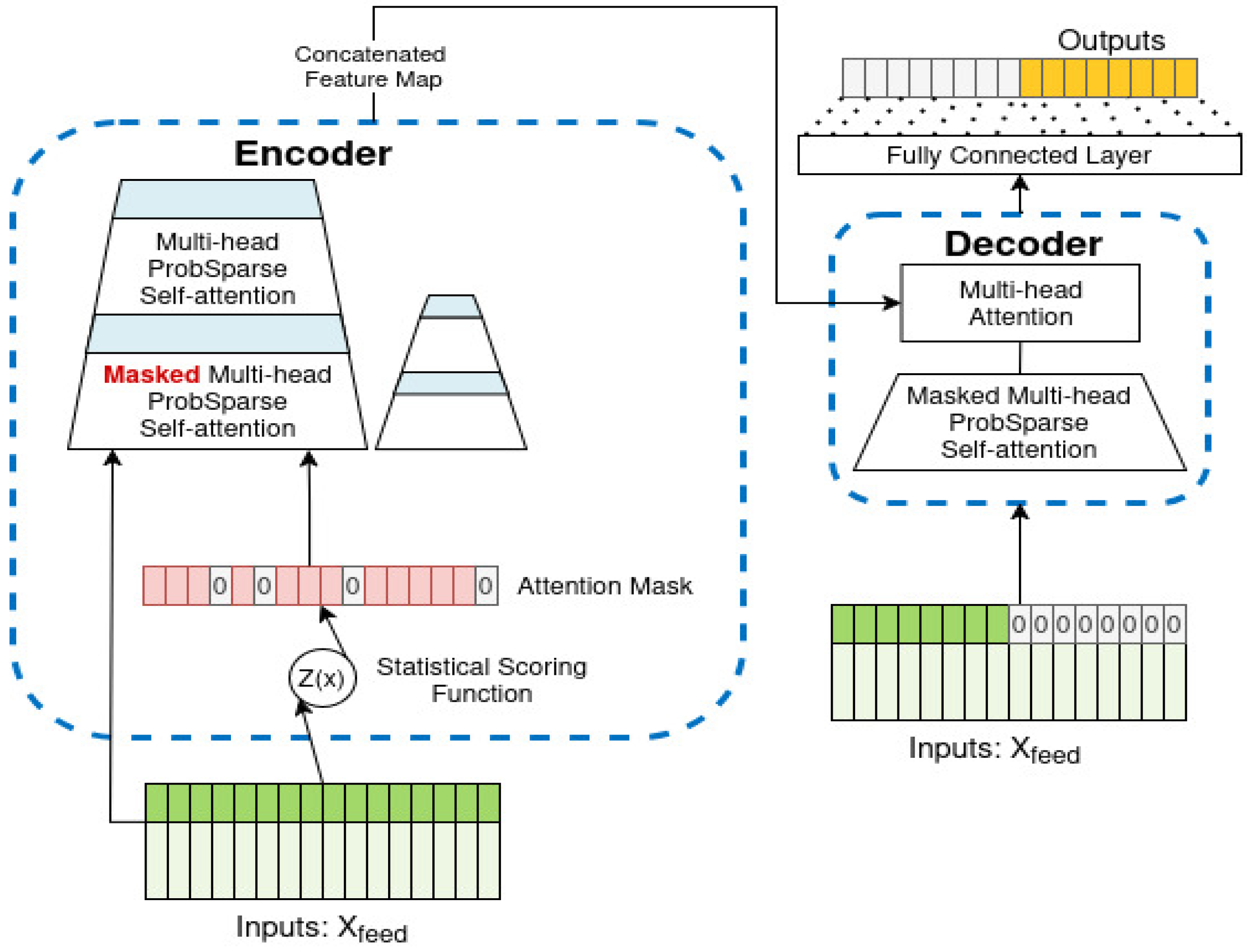
Before delving into the details of the proposed approach, it is important to briefly explain how the AE performs OD. During the training phase, AE focuses on learning normality within any data input. Given a data input x, the encoder transforms it into a latent representation z of lower dimension and passes it to the decoder, which attempts to reconstruct the input x ¯ of the same dimension as x. A reconstruction error is calculated between the input and the estimate x x ¯ , and is back-propagated through the decoder and the encoder, prompting weight readjustment. The proposed method’s skewed training approach factors in the fact that real-world data potentially contains outliers, and performs early detection of extreme values, which are then masked from the encoder in the training phase to improve focus on learning the normal data. As described above, masking is used in the encoder to increase its learning efficiency with the potential of reducing the computational complexity. In decoders, the model is prevented from cheating by masking future values. In this article, the focus is on encoder masking, i.e., identifying outliers in streaming data, not forecasting them. Given this objective, it is reasonable to mask the data based on relevance, which in this case is outlierness. The proposed approach is then to use unsupervised, distribution-free scoring methods with low computational complexity, which are directly applicable to univariate random variables. The data are masked prior to encoding to allow the model to focus on learning which samples are normal. This allows the decoder to reconstruct data based on the learned normality without being influenced by extreme values. The selected statistically based MAD and Chebyshev inequality methods (similar to distribution-free Z-score) meet all these criteria [5]. The model selected for this experiment is the Informer NN model proposed by [18], which is a Transformer for long sequence time series (LSTS). It is characterized by lower complexity than standard Transformers due to its probability-sparse self-attention mechanism. The encoder component is modified by introducing the proposed masking using the three statistical techniques described above. Figure 2 and Figure 3 illustrate both the original Informer and the modification introduced in this paper.
Figure 2 shows that the same data are passed to both the encoder and the decoder. Before passing the data to the encoder, it is processed by an early outlier scoring function (MAD or Chebyshev inequality in this case, denoted in Figure 2, as Z ( x ) ), the result of which are the potential outliers that are masked during the learning phase. The data are then encoded into a larger dimension (i.e., 512) and the output fed into the decoder, which attempts to reconstruct it by reducing the dimensionality back to that of the original input data. From this point on, the reconstruction error (MSE) is calculated for each observation using the original input and the predicted value. It is used as the basis for separating normal from anomalous data in the next part of this experiment.

3.5. The Quasi-Dynamic Threshold Mechanism

After reconstructing the input data X i , a reconstruction error tensor is computed using the MSE as a loss function, applied to the tensor X i and the predicted output X ^ i . The MSE is defined as follows:
MSE = 1 n i = 1 n ( X i X ^ i ) 2 ,
yielding strictly positive reconstruction error, i.e., MSE > 0 . Then, how large should the error be for an observation to be considered anomalous? The answer is found by analyzing the model reconstruction error and defining a sound and objective methodology for drawing the classification boundary between normal and abnormal data, based on the assumption that the larger the error, the higher the risk that the observation is an outlier. A statistical approach to boundary definition based on well-established theory is proposed, with the classification results being compared to the fixed threshold of 95%. Three new thresholding mechanisms are then defined based on the Chebyshev score, robust Z-score, MAD score, and standard Z-score after Box–Cox transformation. These scores are calculated for the overall MSE, and the thresholds are defined based on the expected confidence level. However, due to the data being unlabeled, estimating the performance of these thresholding mechanisms remains a challenge. For this purpose, artificial noise is added to the test data, while the OD performance of the thresholding mechanisms using the same model is estimated using the following five standard model performance metrics: accuracy, precision, recall, F1-score, and AUROC. The method with the highest performance by combining AUROC and recall is considered the most suitable for OD in the given input data. In addition to the detection performance metrics, the model’s computational complexity (time and memory utilization) is also assessed. The proposed model’s performance is compared to relevant models from the literature, namely the long-short-term memory AE (LSTM-AE) and the SARIMA (seasonal auto-regressive integrated moving average), alongside the base Informer model. LSTM-AE is popular for OD in sequential and temporal data [5], and its AE portion uses the reconstruction error like the proposed modified Informer model. SARIMA was selected as a good statistical method candidate for OD in time series data.

3.6. Outlier Voting Mechanism

After the combined masking method and thresholding mechanism are ranked according to their performance, the experimental models with the two highest performance metrics are selected to participate in a vote of outlierness. Any observation is flagged as an outlier if both models detect it as such (logical function AND), or when any of the two models flags it as such (OR). Figure 3 illustrates the end-to-end process from the model prediction output to the outlier classification based on the voting mechanism established on best performing scoring functions (Z-score, MAD, Chebyshev, etc.) using the MSE-based reconstruction errors.

3.7. Computational Complexity

An important consideration when developing a method for detecting anomalies in telecommunications is the trade-off between the detection performance improvement and the associated computational cost for training and testing the model. As part of this experiment, the selected models’ resource consumption in terms of time and memory is measured for both the training and the testing phases. The models’ theoretical requirements as a function O ( · ) of the timeseries’ length T, batch size B, number of features F, depth L, and hidden layers H (for DL models) are summarized in Table 2 below [5]. For SARIMA models, k = p + q + P + Q represents seasonal and non-seasonal orders. The table has three columns, Model containing the list of models used during the experiment and Time Complexity column (respectively, Memory Complexity) containing the function O ( · ) using the above list of parameters, showing how they affect the utilization of time (respectively, memory).
From the table, it can be noted that the number of training iterations (epochs) is not included in the formula since the final metric will be based on one epoch for comparison. Additionally, the SARIMA function indicates a higher complexity in terms of time than memory. For long time series, the Informer is more memory efficient than LSTM-AE due to the quadratic complexity of the LSTM’s number of hidden layers H. On the other hand, for shorter series, LSTM-AE may perform better, depending on H. In terms of memory efficiency, sparse attention increases the Informer’s efficiency, as opposed to LSTM-AE, which stores all activation functions in memory. These observations will be verified by the experimental results.

4. Data Source and Preprocessing

The dataset used in this experiment is an extract of the multi-source urban dataset from Milano and the province of Trentino [19] collected between 1 November 2013 and 1 January 2014, and containing data from five different sources: weather stations, Internet electronic communications, network analysis, geographical information, and cellular devices logs. The telecommunications data have two parts: the first related to human activity and the second to telecommunication interactions within and between locations.
CDR is generated and collected by all major network elements involved in a user’s interaction within a mobile network. The primary HTA included voice calls, SMS messaging, and mobile Internet usage at the time of these data collection.
  • For each of these interactions, a unique identifier is created by the system to trace the end-to-end activity. The communication is initiated by the UE and sent to a base transceiver station (BTS), which connects to the core network.
  • For voice calls and text messages, the traffic is handled by the mobile switching center (MSC).
In the case of SMS, the messages are further routed through the short message service center (SMSC) before being delivered to the MSC, BTS, and finally the recipient’s UE. Calls or messages initiated by the UE will be marked as outgoing, and those received as incoming.
  • For Internet usage, data packets are processed through packet-switched gateways that assign an Internet Protocol (IP) address to the UE that helps track activity and location (region, country), establish a session ID, and connect it to external data networks. Internet usage will be recorded in the volume of data utilized during a session.
Each piece of equipment along the communication path will log its ID in the CDR to mark its participation, as well as the timestamps marking the start and end of the activity treatment by it. Each UE is assigned to geographical grid areas identified by Grid IDs, which are derived from the known radio coverage and locations of the BTS.
Additionally, authentication, billing, and performance monitoring functions are performed by other core network servers. These were not included in this dataset. This paper focuses on anomaly detection in the HTA part of the dataset. It is provided by Telecom Italia and contains CDRs generated by radio base stations (RBS) representing the amount of SMS received or Incoming SMS as “SMSIn”, of Outgoing SMS as “SMSOut”, of Incoming Calls as “CallIn”, of Outgoing Calls as “CallOut”, and of Internet usage as “Internet”, grouped by destination identified by country code, then aggregated at regular 600,000 milliseconds (10 min) time intervals as timestamps. To account for spatial irregularity, data aggregation is performed in regular squared areas called grids, overlaid on Milano and Trentino, named square ID or GridID in the dataset. A predefined function of the RBS coverage area and the grid area is used to estimate the proportion of activity provided by each grid. The final dataset contains close to 320 million records of HTA aggregated every 10 min, over 10,000 grids, grouped by destination.

4.1. Data Preprocessing

Given the large number of grids and the data volume, using the entire dataset was deemed computationally impractical for real-time OD, especially considering that such models would realistically be deployed on devices with limited computational resources. Therefore, 2% of the 10,000 grids were randomly sampled for model training and testing. Only the first 16 days of the data from these sampled grids were used for training, while the remaining samples were reserved for testing of the OD. This spatial sampling and temporal segmentation strategy reduces the computational complexity and prevents model overfitting. The preprocessing procedures are illustrated in Figure 4.
The processed data used for building the model is summarized as follows:
  • The GridID variable was treated as a categorical variable, although denoted as numerical.
  • Timestamp contains time blocks indicating the recorded data. A total of 8920 time blocks of 10 min each are formed.
  • The Destination variable contains categorical variables with 2 values, Local and International.
  • SmsIn, SmsOut, CallIn, CallOut, and Internet are all variables of interest used to detect outliers that contain continuous values.

4.2. Dataset Distribution

The distribution of Internet consumption is bimodal, indicative of 2 sub-groups of usage profiles among the grids. From the time series plot, it is notable that the usage is higher in November, while the traffic level drops from 1 December going forward. The Incoming Calls (CallIn) and Outgoing Calls (CallOut) distributions also show bimodality, but less pronounced than that of the Internet distribution. The drop of traffic level on the time series plot is more pronounced for incoming calls than for outgoing calls, and correlates well with one of the Internet distribution. The Incoming SMS (SmsIn) and the Outgoing SMS (SmsOut) are closer to unimodality, with the latter less smooth than the earlier. Similar drop in traffic level from 1 December until the end of the period.

5. Challenges for Algorithm Implementation

Several challenges were encountered during model training, which motivated the data preprocessing technique and model parameter selection. To reduce the computational cost of the proposed method and to prevent memory leaks, the dataset’s number of features was minimized. Beyond the memory needed to buffer training data, additional resources were required to compute early anomaly-detection scores on mini-batches and process them through the encoder. To mitigate the memory requirements, data sampling by grids was employed as a practical solution. Instead of encoding the destination of telecommunication activity as dummy variables—which would have increased dimensionality—the data were grouped and aggregated by grid regions. Furthermore, larger batches took more time for preprocessing but increased the OD performance for certain transformations like Box–Cox, while smaller batches were faster to process but yielded lower effectiveness. Ultimately, performance considerations took precedence in the case of Box–Cox masking. Overall, the results of the Box–Cox transformed with a Z-score threshold proved to be inadequate as they were invariant. This is explained by the small batch size (i.e., 32) used, which is not enough for proper estimation of the Box–Cox distribution parameter λ . As a result, the outputs from the Box–Cox transformation—when combined with Z-score thresholding—were deemed insufficiently reliable for reporting.
The results across the different features for all models evaluated in this experiment, including the baseline Informer NN from [18] and the proposed modified Informer with different masking and thresholding approaches, are presented in Table 3, Table 4, Table 5, Table 6 and Table 7 and Figure 5, Figure 6, Figure 7 and Figure 8. The LSTM-AE, SARIMA, and the baseline Informer, against which the proposed model’s performance is compared, are accordingly denoted, with the latter being designated as “Baseline Informer”, with blank or “None” in the masking column and with “Standard” in the Threshold column, as no masking was used in this case and thresholding remained fixed and standard.

6. Experimental Results and Discussions

The experiment is conducted on univariate datasets, and the results are organized into Table 4, Table 5 and Table 6. Each of them illustrates the masking mechanism with threshold combinations used for the OD on the first two columns, while the following five columns indicate the NN model performance obtained from the testing based on artificial outlier injection. The contents of the columns are described here:
  • Masking illustrates the corresponding mechanism used on the Informer model, with “None” denoting that no masking was used and therefore representing the base model. Both “MAD” and “Chebyshev” denote the proposed masking methods.
  • Threshold denotes the corresponding mechanisms where “standard” denotes the commonly used 95% threshold, which is compared to that obtained through Chebyshev, Box–Cox, and MAD thresholds.
  • Precision indicates how many of the identified normal data points are correctly recognized.
  • Accuracy is an indicative of how often the model correctly classifies normal data and outliers.
  • Recall represents the model sensitivity at detecting outliers, i.e., how many of the outliers were detected among all known outliers.
  • F1-score illustrates the harmonic mean of the precision and recall, which is a measure of how balanced the model is at classifying both normal data and outliers.
  • AUROC measures the ability of the model to accurately discriminate between the normal data from outliers.
The original data presented in the study and the code for its reproduction are openly available in https://github.com/VOICE-TONE/Outlier-Detection-Based-on-Encoder-Masks-Inflation-and-Quasi-Dynamic-Thresholding, accessed on 22 October 2025. The simulations were run on a computer equipped with an Intel Core i9-13900KF Processor at 3.00 GHz, 64 GB of random access memory (RAM), a solid-state drive (SSD), and an NVIDIA GeForce RTX 4070 (12 GB) graphical processing unit (GPU), Python 3.12.4, and Torch 2.5.

6.1. Computational Complexity Comparison

During the training and testing phases, the corresponding time and memory complexity of each model were measured (Table 3). It is to be noted that the memory during the testing phase remains high since the full model is still stored until the classification is completed. The best and second-best results are highlighted in green and orange, respectively. The modified Informer model did not degrade the baseline Informer’s computational efficiency, while achieving notable performance improvement as described below. This may be explained by the fact that the statistical scoring is calculated for each batch passed to the encoder, thus compensating for the additional operations in the proposed model. The data sample size is different for each model due to the various training approaches’ applicability. Both Informer models were trained using a 1% sample of the entire dataset, which contains all grids. In contrast, for LSTM-AE and SARIMA, the models were trained for each telecommunication grid in the dataset and applied to the future samples of the same grid. Regarding the SARIMA model, only 2 grids were used due to its theoretical complexity, as explained in the previous Section. Hence, for the first 16 days of the samples used for training, a grid with its full 10-minute data increment would have 2304 data points, which is why the training and testing sample sizes are not exactly the same across the Informer NN and the other two models. Furthermore, the SARIMA was restricted to the auto-regressive model and seasonality, based on the partial auto-correlation function results. The SARIMA parameters used were therefore, p = 1 , d = 0 , q = 0 , P = 1 , D = 0 , Q = 0 , S = 144 where 144 represents daily seasonality steps. The number of features per sample is also outlined in the Table 3, and the training and prediction times are calculated both per sample and per feature for all four models.
The results indicate that SARIMA has nearly 16 times higher memory requirements than the proposed model (or the baseline Informer), while the memory cost of LSTM-AE is 1.8 times higher. The training time for SARIMA and LSTM-AE is also over 27 times longer; however, when it comes to testing, all four models have similar performance. As for the testing (or inference) time, the proposed Informer is only slightly slower than the LSTM-AE but is 34% more efficient than the SARIMA. The modified Informer does not have higher computational complexity than the base model because the masking and thresholding methods employ a probability-sparse self-attention mechanism as described in Section 3.4.

6.2. Comparison of Classification Performance for OD

The results of the Internet data in Table 4 show that the best OD classification performance based on AUROC is obtained by employing the MAD threshold in both the Informer baseline with an AUROC of 87.0% followed by the modified MAD masking model with a very close AUROC of 86.4%. Both combinations of masking and thresholding achieve high accuracy (> 75.0 % and recall (99.8% and 98.2%, respectively). However, the precision remains poor, less than 20%. Both models are characterized by precision and F1-score that result in many false positive detections. SARIMA achieves the highest F1-score (41.3%) and precision (40.5%), both at least 15.0% higher than the other models, but with a much lower recall (42.2%). These results indicate that SARIMA generates fewer false positive detections than other models. Throughout this Section, the best and second-best results are highlighted in green and orange, respectively, but only for the F1-score and AUROC metrics because they are the most reliable metrics for OD, as the data are usually characterized with very high variation. The highest accuracy is obtained by the modified Informer with MAD masking and Chebyshev thresholding; however, such high accuracy is not conclusive given the precision. The highest recall is obtained through the Chebyshev masking and MAD thresholding. Overall, thresholding exhibits a strong effect on anomaly classification in the Internet data; however, there is notably poor precision. The same applies to the LSTM-AE model.
In Table 5, for Incoming Calls, the highest recall (100%) is obtained by the Informer models, regardless of the thresholding mechanism selected, but once again at the cost of precision, which is still poor (less than 20%). With an AUROC of 89.6% and a F1-score of 26.6%, the modified Informer model combined with MAD thresholding outperforms the other models at OD and classes separation, with an 80% accuracy, but at a cost of the precision, which remains very low. The highest precision is achieved by SARIMA, which also yields the best accuracy (94.8%) and the F1 score (47.6%), but performs poorly in OD with a recall lower than 50%, with MAD thresholding and Chebyshev masking resulting in a slightly lower AUROC (85.2%).
For outgoing calls, the modified Informer model using the combination of MAD masking and MAD thresholding, provides the highest recall (100%) and AUROC of 86.5%, as well as a reasonably high accuracy of 74.0%, but a very low precision (12.2%) and F1-score (21.8%), indicative of its poor sensitivity. The precision (12.2%) and F1-score (21.8%) remain significantly lower than SARIMA with a precision of 35.3% and an accuracy of 36.0%. The overall precision remains low at under 50% indicating the methods’ poor ability to identify false positives. SARIMA obtains the highest F1-score for both data types, but at a significant memory cost, while its AUROC is about 10% lower than the Informer models. The LSTM-AE results are close to those obtained for both the baseline and modified Informer.
Table 6 shows that for both Incoming SMS and Outgoing SMS, LSTM-AE is slightly better than the proposed model at separating anomalies from normal data based on the AUROC and F1-score metrics. The modified model with MAD masking is superior at separating classes with a recall of 100% and a reasonably high AUROC of 85.5% for Incoming and 86.6% for Outgoing SMS. However, a 0% precision is recoded for this, the MAD masking combined with Chebyshev or Standard thresholds, which indicates that there is a feature of the data that is not suitable for the introduced masking approaches. SARIMA obtains marginally higher accuracy than the proposed model with combined Chebyshev masking and thresholding for the Incoming SMS, while the latter is best performing for the outgoing SMS. The combination of MAD masking and MAD thresholding achieves 100% recall, with the second highest AUROC of 85.5%. Overall, the precision remains below 50% in all cases, with the SARIMA reaching 48.3% and 46.3% for Incoming and Outgoing SMS, respectively. The proposed model is still beneficial, considering the much higher memory requirements of both LSTM-AE and SARIMA.

6.3. Influence of Masking and Thresholding on the Performance

Based on the above, AUROC is considered to be the best metric for estimating the model’s performance. Figure 5 shows the median change in AUROC between the base model without masking and the model on which the Cheyshev and MAD masking have been applied, by input feature. This suggests a clear dominance of the models with masking techniques over the base Informer model for the Incoming Calls and the Internet features, with the largest difference of 11.1% obtained for the latter. Both masking techniques underperformed on the Incoming SMS data, with the lowest performance achieved by MAD masking (−12%). Chebyshev masking also performed well on Outgoing SMS data and had comparable performance to that of the base model. This variability in results is visible in Figure 6 showing a higher median AUROC for models using masking versus the baseline model. The results indicate a positive effect of masking on the performance metric with a median value of 57.8% of model with masking versus 52% for those without masking, making a median increase of 5.8%, as shown in Figure 6.
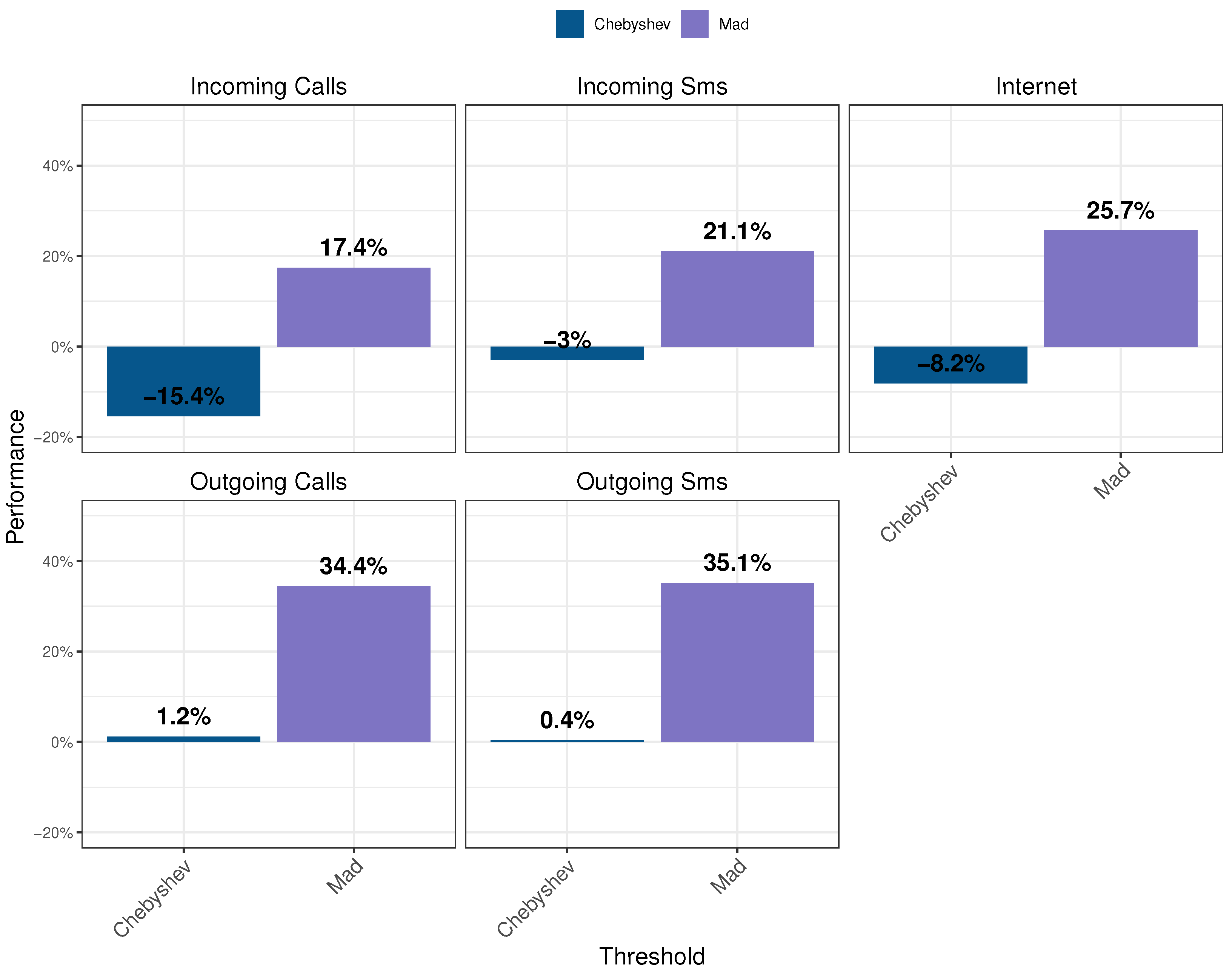
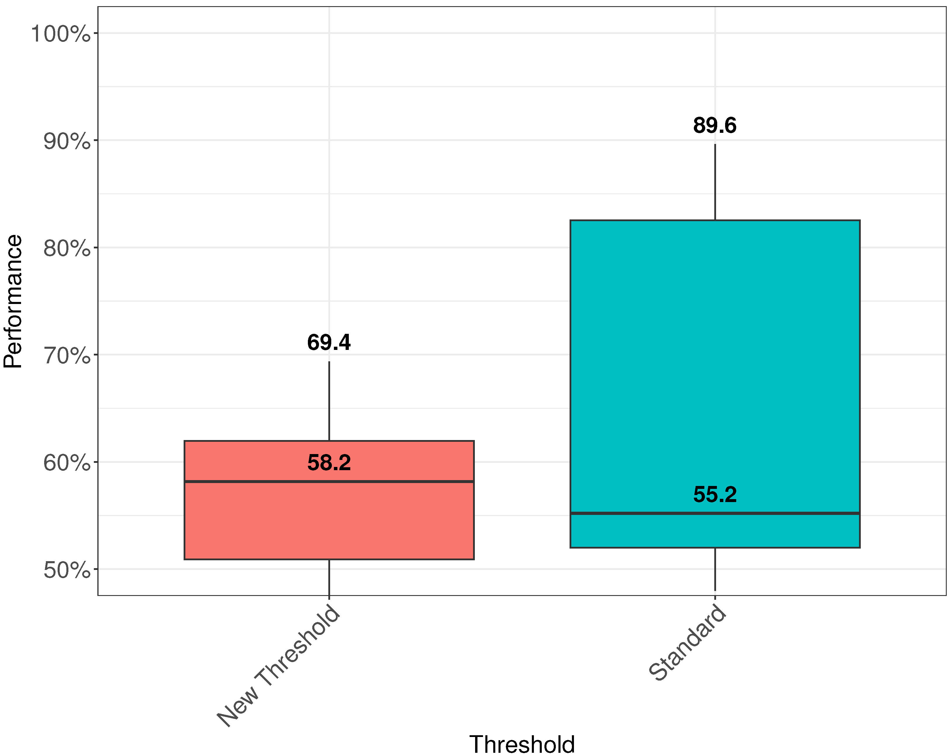
The proposed thresholding exhibits a larger increase in AUROC, especially when using the MAD thresholding mechanism versus the standard threshold as per Figure 7. The difference varies from 17.4% for the Incoming calls feature to close to 35% for both the Outgoing Calls and SMS. Chebyshev thresholding underperforms for all data types. When analyzing the overall performance of models on which statistical thresholding was applied versus the standard 95% threshold, the median difference is about 3% with the proposed thresholding superseding the standard one. The overall effect of thresholding on the model’s performance is presented in Figure 8 showing that the median performance of the proposed thresholding is up to 3% higher than the baseline. The latter has more variability than the former, which in some cases indicates a better performance.

Regression Analysis of the Influence of Masking and Thresholding

To better assess the combined effect of masking and thresholding on the AUROC, a linear regression analysis was performed, using the model, the masking type, and the thresholding mechanism as predictors of the AUROC with an interaction term between the masking and thresholding. The results show an adjusted R 2 of 0.884 indicating that the selected models explain 88.4% of the AUROC’s variability with a very high significance estimated by the p-value which is the probability of obtaining a value greater than the one set under the null hypothesis that there is no difference between the models (which is equivalent to the regression coefficients are all being equal to 0). Essentially, the null hypothesis H 0 : β 1 = β 2 = = β k , where β 1 β k represent the estimated effects of the various model combinations to the prediction of the AUROC, while the alternate hypothesis is H A : At least one β j 0 , where the p-value represents the probability P of the model’s effect to be as extreme as the one observed in the results given the null hypothesis p - value = P F F model | H 0 , which indicates the model significance. Table 7 shows the results of the regression analysis.
The Method column contains the masking and the thresholding methods, or the cases when they are implemented together. The column Estimate records the effect size of each method on the AUROC performance, with the sign of the estimate indicating the direction of the correlation. The Standard Error column shows the error used to compute the lower and upper boundaries, respectively, recorded in the columns Lower Estimate and Upper Estimate. The p -value column shows the regression p-values used to measure the importance of the method in influencing the model’s performance. The Significance column uses the p-values and the following levels as cutoff values to classify the results. The value is considered “Very strong” if the p-value is < 0.05 (or 5%), “Strong” if the significance is between 5 and 10%, “Weak” if the p-value is between 10 and 30%, “Very weak” if p [ 30 ; 50 % ] , and “None” being equivalent to “Non-significant” if the p-value is higher than 50%. The intercept case (first row) is very important as it indicates the base detection performance of the model. MAD thresholding has the strongest significance and solely contributes to an increase of AUROC by 31%. The significance of MAD masking is strong but reduces the AUROC by nearly 6%. The best combination of the two approaches is obtained for MAD masking and thresholding, improving the AUROC by 10.6%. When no masking is used with MAD thresholding, the AUROC increases by almost 4%. These results of the regression analysis confirm the superiority of the MAD thresholding and masking approaches for streaming cellular data.

7. Conclusions

This paper explores the effect of encoder masking on OD performance when using an AE-based Informer NN on unlabeled HTA time series data. It also introduces a state-of-the-art statistical thresholding approach applicable to model the output reconstruction error to make the final separation between normal data and outliers. In addition, it compares the computational efficiency of the model to the baseline AE, LSTM-AE, and SARIMA models at detecting outliers in the same data. The experimental results indicate that:
  • Encoder masking improves the baseline Informer detection accuracy without degrading the proposed model’s computational complexity or memory requirements. Its training data processing speed is comparable to that of the LSTM-AE and SARIMA models, while incorporating the knowledge provided by the increased number of data features, and providing significantly higher memory efficiency. Consequently, the modified Informer is suitable for implementing OD functionality in the near-real-time RIC, and as observed by the authors of [20], it is viable for implementation in cases when OD in under 10 ms is required, as is also the case for the proposed model. The OD can be implemented via an xApp running on the RIC to detect malicious traffic and prevent it from exploiting security vulnerabilities in other xApps that could result in denial of service. Future work will further investigate the OD through real-time experiments in O-RAN.
  • Statistical thresholding yields better results at separating classes of data and may be used together with the output of the DL model’s loss function. It achieves better classification of unlabeled data than using a fixed threshold, e.g., the 95th percentile, which is a conservative value. The proposed thresholding approach adapts this value according to the reconstruction error produced by the model. The combination of MAD thresholding and masking has been shown to yield the most significant improvement in the AUROC.
The results highlight several opportunities for enhancing AE-based learning for OD through effective combinations of masking and thresholding techniques. The present experiments were limited to univariate data streams without extending to multivariate analysis. The latter requires adaptation to cases of global anomaly detection from multiple components streaming data in parallel, such as interference between multiple cells within a grid, affecting only some of the users. Another limitation of the model is that it is designed to be pretrained on previous data windows and not to be retrained on the fly. In future work, the proposed method will be applied to streaming data with evolving distributions. Furthermore, the method requires a user-defined data segment length for the training phase and a fixed window size for estimating the masks using statistical functions, as well as predicting the outliers, which might affect the performance of the model, especially for data with variable data arrival rates. A specific use case could be a partial or total outage of the RAN, causing a consistent reduction in the data arrival. This might impact the ability of the model to properly estimate the mask due to the much smaller sample size received during the outage. Adapting the model to handle this real-world scenario is to be considered in future improvements. Due to the size of the dataset and the memory-intensive nature of the selected models, sampling and data aggregation were employed during preprocessing to mitigate memory leaks. An interesting direction for further investigation involves conducting a sensitivity analysis to determine the optimal sample size beyond which further gains in detection accuracy may not justify the added computational cost. Additionally, extending these methods to multivariate datasets and distributed sensor networks presents a promising avenue for research. In particular, further exploration in this direction will be focused on distinguishing between local OD for individual IoT devices and global OD under edge computing constraints.

Author Contributions

Conceptualization, R.N.M., A.V. and N.G.; methodology, R.N.M., A.V. and N.G.; software, R.N.M., A.V., N.G. and A.I.; investigation, R.N.M., A.V. and A.I.; formal analysis, R.N.M., A.V. and A.I.; writing—original draft preparation, R.N.M. and A.I.; writing—review and editing, V.P., P.K. and A.M.; verification, A.V., P.K., V.P. and A.M.; supervision, P.K. and V.P.; project administration, A.M.; funding acquisition, V.P. and A.M. All authors have read and agreed to the published version of the manuscript.

Funding

This research is funded by the European Union-Next Generation EU, through the National Recovery and Resilience Plan of the Republic of Bulgaria, project No BG-RRP-2.004-0005: “Improving the research capacity and quality to achieve international recognition and resilience of TU-Sofia” (IDEAS) and performed with the support of the Intelligent Communication Infrastructures Laboratory at the “Research and Development and Innovation Consortium”, Sofia, Bulgaria.

Institutional Review Board Statement

Not applicable.

Data Availability Statement

The original data presented in the study and the code for its reproduction are openly available in https://github.com/VOICE-TONE/Outlier-Detection-Based-on-Encoder-Masks-Inflation-and-Quasi-Dynamic-Thresholding, accessed on 22 October 2025.

Acknowledgments

The authors acknowledge the support of Polya Georgieva in providing materials that gave useful insights into the design of the mask inflation in the proposed method. During the preparation of this manuscript, the authors used Gemini 2.5 Flash for the purposes of LaTeX formatting of the tables and generating some entries in the list of references. The authors have reviewed and edited the output and take full responsibility for the content of this publication.

Conflicts of Interest

The authors declare no conflicts of interest.

Abbreviations

The following abbreviations are used in this manuscript:
5GFifth Generation
AEAutoencoder
ARIMAAuto-regressive Integrated Moving Average
AUCArea Under the Curve
AUROCArea Under the Receiver Operating Characteristic
CDRCalls Detailed Records
CNCore Network
CNNConvolutional Neural Network
CNN-AEConvolutional Neural Network Autoencoder
DBSCANDensity-Based Spatial Clustering of Applications with Noise
DLDeep Learning
GANGenerative Adversarial Networks
GMMGaussian Mixture Model
HTAHuman Telecommunications Activities
LSTSLong Sequence Time Series
LSTMLong-Short-Term Memory
LSTM-AELong Short-Term Memory Autoencoder
MADMedian Absolute Deviation
MSEMean Square Error
NNNeural Network
O-RANOpen Radio Access Network
ODOutlier Detection
OODOut-of-Distribution
PDFProbability Density Function
RANRadio Access Network
RICRAN Intelligent Controller
SARIMASeasonal Auto-Regressive Integrated Moving Average
UEUser Equipment
WBSWireless Base Stations

References

  1. Giordani, M.; Polese, M.; Mezzavilla, M.; Rangan, S.; Zorzi, M. Toward 6G networks: Use cases and technologies. IEEE Commun. Mag. 2020, 58, 55–61. [Google Scholar] [CrossRef]
  2. Edozie, E.; Shuaibu, A.N.; Sadiq, B.O.; John, U.K. Artificial intelligence advances in anomaly detection for telecom networks. Artif. Intell. Rev. 2025, 58, 100. [Google Scholar] [CrossRef]
  3. Aziz, Z.; Bestak, R. Modeling Voice Traffic Patterns for Anomaly Detection and Prediction in Cellular Networks based on CDR Data. IEEE Trans. Mob. Comput. 2024, 23, 13131–13143. [Google Scholar] [CrossRef]
  4. Mahrez, Z.; Driss, M.B.; Sabir, E.; Saad, W.; Driouch, E. Benchmarking of anomaly detection techniques in o-ran for handover optimization. In Proceedings of the 2023 International Wireless Communications and Mobile Computing (IWCMC), Marrakesh, Morocco, 19–23 June 2023; pp. 119–125. [Google Scholar]
  5. Mfondoum, R.; Ivanov, A.; Koleva, P.; Poulkov, V.; Manolova, A. Outlier Detection in Streaming Data for Telecommunications and Industrial Applications: A Survey. Electronics 2024, 13, 3339. [Google Scholar] [CrossRef]
  6. Rassam, M.A. Autoencoder-Based Neural Network Model for Anomaly Detection in Wireless Body Area Networks. IoT 2024, 5, 852–870. [Google Scholar] [CrossRef]
  7. Owoh, N.; Riley, J.; Ashawa, M.; Hosseinzadeh, S.; Philip, A.; Osamor, J. An Adaptive Temporal Convolutional Network Autoencoder for Malicious Data Detection in Mobile Crowd Sensing. Sensors 2024, 24, 2353. [Google Scholar] [CrossRef] [PubMed]
  8. Hua, X.; Zhu, L.; Zhang, S.; Li, Z.; Wang, S.; Deng, C.; Feng, J.; Zhang, Z.; Wu, W. GenAD: General unsupervised anomaly detection using multivariate time series for large-scale wireless base stations. Electron. Lett. 2023, 59, e12683. [Google Scholar] [CrossRef]
  9. Aziz, Z.; Bestak, R. Insight into Anomaly Detection and Prediction and Mobile Network Security Enhancement Leveraging K-Means Clustering on Call Detail Records. Sensors 2024, 24, 1716. [Google Scholar] [CrossRef] [PubMed]
  10. Rafique, S.H.; Abdallah, A.; Musa, N.S.; Murugan, T. Machine learning and deep learning techniques for internet of things network anomaly detection—Current research trends. Sensors 2024, 24, 1968. [Google Scholar] [CrossRef] [PubMed]
  11. Kim, J.; Kang, H.; Kang, P. Time-series anomaly detection with stacked Transformer representations and 1D convolutional network. Eng. Appl. Artif. Intell. 2023, 120, 105964. [Google Scholar] [CrossRef]
  12. Mo, Y.; Fu, H.; Bai, S.; Deng, C.; Tang, T.; Lang, J.; Zhou, F. InfoFlow: A Transformer-based Time Series Anomaly Detection Model with Information Bottleneck and Normalizing Flows. arXiv 2024, arXiv:2402.00000. [Google Scholar]
  13. Zhang, Y.; Hu, J.; Wen, D.; Deng, W. Unsupervised evaluation for out-of-distribution detection. Pattern Recognition 2024, 160, 111212. [Google Scholar] [CrossRef]
  14. Sultan, K.; Ali, H.; Zhang, Z. Call detail records driven anomaly detection and traffic prediction in mobile cellular networks. IEEE Access 2018, 6, 41728–41737. [Google Scholar] [CrossRef]
  15. Priyadarshini, I.; Alkhayyat, A.; Gehlot, A.; Kumar, R. Time series analysis and anomaly detection for trustworthy smart homes. Comput. Electr. Eng. 2022, 102, 108193. [Google Scholar] [CrossRef]
  16. Chebyshev, P. Des valeurs moyennes. J. Math. Pures Appl. 1867, 12, 177–184. [Google Scholar]
  17. Stellato, B.; Van Parys, B.; Goulart, P. Multivariate Chebyshev inequality with estimated mean and variance. Am. Stat. 2017, 71, 123–127. [Google Scholar] [CrossRef]
  18. Zhou, H.; Li, J.; Zhang, S.; Zhang, S.; Yan, M.; Xiong, H. Expanding the prediction capacity in long sequence time-series forecasting. Artif. Intell. 2023, 318, 103886. [Google Scholar] [CrossRef]
  19. Barlacchi, G.; De Nadai, M.; Larcher, R.; Casella, A.; Chitic, C.; Torrisi, G.; Antonelli, F.; Vespignani, A.; Pentland, A.; Lepri, B. A multi-source dataset of urban life in the city of Milan and the Province of Trentino. Sci. Data 2015, 2, 150055. [Google Scholar] [CrossRef] [PubMed]
  20. Hung, C.F.; Tseng, C.H.; Cheng, S.M. Anomaly Detection for Mitigating xApp and E2 Interface Threats in O-RAN Near-RT RIC. IEEE Open J. Commun. Soc. 2025, 6, 1682–1694. [Google Scholar] [CrossRef]
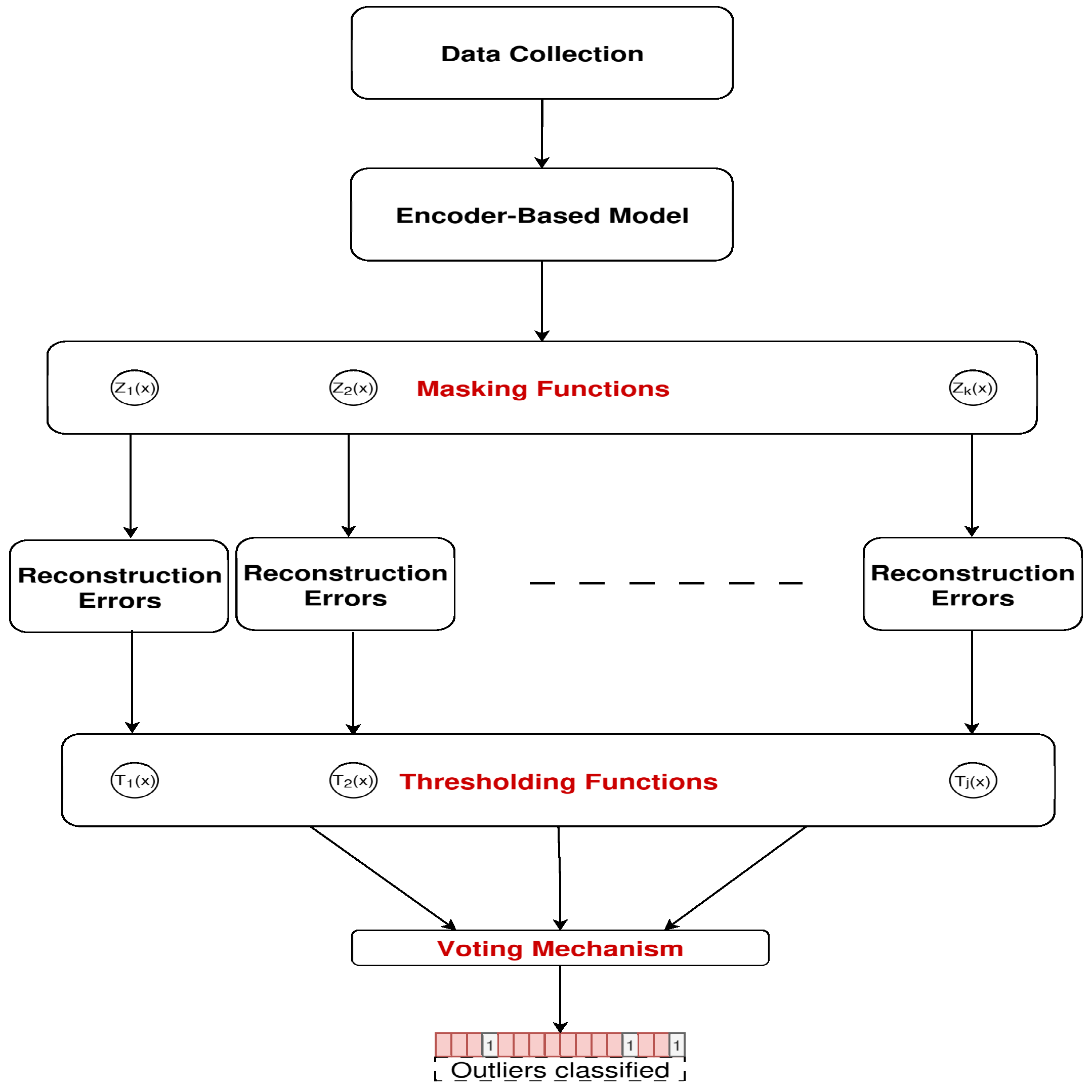
Figure 1. A diagram of the proposed method’s operation.
Telecom 06 00084 g001
Figure 2. Modified Informer NN with Encoder Attention Mask Inflation.
Telecom 06 00084 g002
Figure 3. Model selection, outlier scoring, and voting mechanism.
Telecom 06 00084 g003
Figure 4. Data preprocessing procedures.
Telecom 06 00084 g004
Figure 5. Change in AUROC performance for the different masking techniques by feature.
Telecom 06 00084 g005
Figure 6. Overall masking effect on performance metrics.
Telecom 06 00084 g006
Figure 7. Change in AUROC performance for the different threshold techniques by feature.
Telecom 06 00084 g007
Figure 8. Overall threshold effect on performance metrics.
Telecom 06 00084 g008
Table 2. Theoretical time and memory complexity for all models.
ModelTime ComplexityMemory Requirements
LSTM Autoencoder O ( 2 L · T · H ( H + F ) ) O ( 2 L · T · H + H ( H + F ) )
SARIMA O ( F · T · k 2 ) O ( F · T )
Baseline Informer O ( L · T log T · H ) O ( L · T log T · H + H 2 )
Modified Informer O ( L · T log T · H + B ) O ( L · T log T · H + H 2 + B )
Table 3. Resource usage and performance comparison across models. The best and second-best results are highlighted in green and orange, respectively.
MetricBaseline InformerModified InformerLSTM-AESARIMA
Training Time Per Sample Per Feature (ms)0.110.112.9923.74
Testing Time Per Sample Per Feature (ms)0.0550.0550.0470.074
Peak Memory during Training (MB)718.50718.501293.7912,026.81
Peak Memory during Testing (MB)7197191198.1912,029.56
Training Size57,60057,60028,2244608
Test Size13,82413,82425,3444608
Number of Features5531
Training Execution Time (s)31.6831.68253.17109.39
Testing Execution Time (s)3.83.83.570.34
Table 4. Comparative OD performance between the proposed Modified Informer and baseline models for Internet data. The best and second-best results are highlighted in green and orange, respectively.
ModelMaskingThresholdPrecisionAccuracyRecallF1-ScoreAUROC
LSTM-AENoneStandard15.0%60.5%86.0%24.3%82.9%
SARIMANoneStandard40.5%94.2%42.2%41.3%83.1%
Baseline
Informer
-Standard19.0%93.4%25.6%21.8%60.8%
Chebyshev9.1%94.3%6.4%7.5%52.0%
MAD12.7%75.1%99.8%22.5%87.0%
Modified
Informer
MADStandard14.3%92.9%19.2%16.4%57.4%
Chebyshev16.7%95.5%6.4%9.6%52.6%
MAD12.7%75.5%98.2%22.5%86.4%
Modified
Informer
ChebyshevStandard22.5%93.7%30.2%25.8%63.1%
Chebyshev21.4%93.5%30.2%25.0%63.0%
MAD9.1%63.8%100.0%16.7%81.2%
Table 5. Comparative OD performance between the proposed Modified Informer and baseline models for Calls usage data. The best and second-best results are highlighted in green and orange, respectively.
ModelMaskingThresholdIncoming CallsOutgoing Calls
Precision Accuracy Recall F1-Score AUROC Precision Accuracy Recall F1-Score AUROC
LSTM-AENoneStandard13.0%60.0%85.9%21.7%81.8%15.7%60.6%85.4%25.2%75.7%
SARIMANoneStandard46.6%94.8%48.7%47.6%78.5%35.3%93.7%36.7%36.0%78.9%
Baseline
Informer
NoneStandard15.3%93.0%20.6%17.6%58.2%4.8%92.0%6.4%5.5%50.8%
Chebyshev0.0%93.8%0.0%0.0%48.7%9.1%94.3%6.4%7.5%52.0%
MAD11.0%70.7%100.0%19.8%84.8%12.8%76.8%93.6%22.6%86.8%
Modified
Informer
MADStandard31.4%94.6%42.2%36.0%69.4%6.4%92.1%8.6%7.3%51.9%
Chebyshev9.1%94.3%6.4%7.5%52.0%3.1%94.3%2.2%2.6%49.8%
MAD11.0%70.7%100.0%19.8%84.8%12.2%74.0%100.0%21.8%86.8%
Modified
Informer
ChebyshevStandard28.6%94.3%38.4%32.8%67.4%4.8%92.0%6.4%5.5%50.8%
Chebyshev9.1%94.3%6.4%7.5%52.0%9.1%94.3%6.4%7.5%52.0%
MAD15.3%80.0%100.0%26.6%89.6%11.3%71.7%99.8%20.3%85.2%
Table 6. Comparative OD performance between the proposed Modified Informer and baseline models for SMS usage data. The best and second-best results are highlighted in green and orange, respectively.
ModelMaskingThresholdIncoming SMSOutgoing SMS
Precision Accuracy Recall F1-Score AUROC Precision Accuracy Recall F1-Score AUROC
LSTM-AE-Standard18.0%70.3%86.0%28.9%91.5%15.2%62.0%87.0%24.7%87.1%
SARIMANoneStandard47.4%94.9%49.3%48.3%76.1%45.3%94.7%47.5%46.3%80.6%
Baseline
Informer
-Standard22.5%93.7%30.2%25.8%63.1%5.1%92.0%6.8%5.8%51.0%
Chebyshev21.4%93.5%30.2%25.1%63.0%5.9%92.7%6.8%6.3%51.4%
MAD9.1%63.8%100.0%16.7%81.8%11.9%73.3%100.0%21.3%86.1%
Modified
Informer
MADStandard4.8%92.0%6.4%5.5%50.8%0.0%91.5%0.0%0.0%47.5%
Chebyshev5.3%92.4%6.4%5.8%51.0%0.0%92.7%0.0%0.0%48.1%
MAD11.5%72.1%100.0%20.6%85.5%12.3%74.2%100.0%21.9%86.6%
Modified
Informer
ChebyshevStandard19.0%93.4%25.6%21.8%60.8%19.0%93.4%25.6%21.8%60.8%
Chebyshev16.7%93.6%19.2%17.8%57.8%25.0%95.0%25.6%22.7%58.5%
MAD9.4%65.0%100.0%17.1%81.8%9.8%66.8%9.8%17.9%82.8%
Table 7. Regression analysis of masking and thresholding effects on AUROC. The methods with strong influence are emphasized in bold.
MethodEstimateStandard ErrorLower EstimateUpper Estimatep-ValueSignificance
Intercept Case0.53130.05640.43860.62410.0000Very strong
MAD Masking−0.05960.0301−0.1092−0.01000.0538Strong
Baseline (No Masking)−0.03250.0306−0.09210.01700.2858Weak
Chebyshev Threshold0.03530.0603−0.08380.15450.5666None
MAD Threshold0.31000.06030.19140.42860.0000Very strong
Standard (95%) Threshold0.07440.0603−0.04300.17360.2234Weak
Z-score Threshold0.03510.0522−0.06880.12100.5047None
MAD Masking + Chebyshev Threshold−0.00360.0604−0.12190.11470.9544None
No Masking + Chebyshev Threshold0.00240.0604−0.11710.12191.0000None
MAD Masking + MAD Threshold0.10640.0604−0.01200.22480.0954Strong
No Masking + MAD Threshold0.03940.0426−0.04510.12380.3545Very weak
MAD Masking + Standard (95%) Threshold0.01120.0604−0.10690.12920.8507None
No Masking + Standard (95%) Threshold−0.00540.0426−0.07560.06470.8992None
Disclaimer/Publisher’s Note: The statements, opinions and data contained in all publications are solely those of the individual author(s) and contributor(s) and not of MDPI and/or the editor(s). MDPI and/or the editor(s) disclaim responsibility for any injury to people or property resulting from any ideas, methods, instructions or products referred to in the content.