Abstract
To ensure the on-orbit safety of crewed spacecraft and avoid the threat of constellations such as Starlink to manned spacecraft, the industry has started to research equipping phased array radars for situational awareness of collision threat. In order to enhance the resource allocation capability of the space station’s protection radar system, this paper proposes a task scheduling method based on time shifting constraints and pulse interleaving. The time shifting constraint is designed to minimize the deviation between the actual execution and the desired execution time of the task, and it is negatively correlated with the threat degree of the target. Pulse interleaving is intended to utilize the idle time between the transmitted pulse and the received pulse of a task to perform other tasks, thereby improving the utilization of radar resources. Through computer simulation under typical parameters, our proposed method reduces the average time shifting ratio by about 60% compared to traditional task scheduling methods, and the scheduling success ratio is also higher than that of traditional scheduling methods. This demonstrates the effectiveness of the proposed method in enhancing scheduling efficiency and overall system performance.
1. Introduction
With the rapid deployment of commercial satellite constellations [1], the number of satellites has increased dramatically. These large-scale satellite networks not only occupy valuable space resources but also pose a significant threat to the safe operation of China’s space station. Issues such as the frequent orbital adjustments of satellites, collisions due to satellite malfunctions, and potential space debris [2,3,4,5] have made the task of protecting the space station increasingly challenging. Although we have taken a series of measures to protect the safe operation of the space station, the existing protective measures are no longer adequate in the face of an increasingly complex space environment, especially given unexpected situations such as satellite failures.
Phased array radar (PAR), also known as electric scanning radar, has a beam agility ability [6,7,8,9] and can quickly complete the search and tracking of multiple targets; thus, it has been widely used. However, with the continuous increase in the number of satellites and space debris, the operational burden on phased array radar systems has significantly escalated. How to achieve the efficient and accurate tracking of multiple high-threat targets with limited radar resources has become a key issue that urgently needs to be addressed [10].
The mainstream method for resource scheduling currently is the adaptive scheduling method, which selects the optimal task execution sequence for a given scheduling interval while satisfying radar system resource constraints [11]. Many scholars have conducted in-depth research on the adaptive scheduling method. Reference [12] proposed a scheduling algorithm based on dynamic three-way decision-making, assigning different weights to different threat domains to enable more rational allocation of radar time resources during the tracking phase; reference [13] proposed a scheduling method based on particle swarm annealing algorithm, which has global search capability; However, these algorithms primarily focus on selecting scheduling moments based on the radar tasks themselves, which may lead to insufficient time utilization and the existence of idle time resources. References [14,15,16,17] use a time pointer to point to the current working time of the radar. Based on a certain scheduling criterion, the most suitable task to be executed at the current time is selected for scheduling, and then the pointer slides to the end time of the task, making better use of time resources. Therefore, this algorithm is widely used in task scheduling. However, these algorithms do not utilize the time resources during the radar task’s waiting period, and there is a significant deviation between the actual execution time and the expected execution time of radar tasks, leading to a high time shifting ratio (TSR) [18]. Especially for tracking tasks, the occurrence of time shifting can cause the true position of the target to gradually deviate from the predicted position, resulting in a decrease in tracking accuracy.
Although pulse interleaving and time-pointer-based scheduling have both been studied in radar task scheduling, they are typically applied separately to different types of tasks. The novelty of this paper lies in integrating the two into a unified scheduling framework. The time-pointer scheduling is used to dynamically determine the execution order of tasks, while pulse interleaving is employed to fully utilize the idle periods between the transmission and reception phases of radar tasks, enabling flexible and efficient scheduling under resource-constrained conditions. In addition, a time-shifting constraint is introduced to limit the deviation of actual task execution times from their expected times, thereby ensuring more stable scheduling of high-priority tasks. Compared with existing multi-objective scheduling algorithms, which often focus on a single optimization goal such as maximizing task execution rate or resource utilization, our method achieves a more balanced trade-off among execution timing, priority enforcement, and time-slot utilization. This approach—combining established techniques and enhancing them with a time-shifting mechanism—is specifically designed for highly constrained and complex scheduling scenarios and has not been adequately addressed in the existing literature. Therefore, our main contributions are summarized as follows:
- The integration of time pointer and pulse interleaving algorithms. The time pointer scheduling approach enables the scheduling system to dynamically select and execute the next optimal task based on the current radar’s operating status and task queue conditions, typically prioritizing tasks according to their urgency. The pulse interleaving technique further refines the execution gaps between tasks. By inserting additional tasks during the idle periods between radar transmission and signal reception, it increases the density of task execution, thereby optimizing the overall task execution efficiency without compromising high-priority tasks.
- The introduction of time shifting constraints. By strictly controlling the deviation between the actual execution time and the expected execution time of tasks, the scheduling system can avoid significant deviations in the task execution time and reduce the risk of task failure or performance degradation caused by excessive time shifts. It also enables the scheduling system to allocate radar resources more reasonably, ensuring that tasks aiming at high-threat targets can be prioritized and executed accurately while not ignoring the needs of other tasks.
- Enhancing the on-orbit safety of space stations. The method proposed in this paper augments the radar system’s processing capability in multi-task environments, effectively addressing the complexities of the space environment surrounding space stations. It ensures that, when tracking high-speed, high-threat targets, the deviation between predicted and actual positions remains within a controllable range, thereby improving tracking accuracy and reliability and ultimately bolstering the on-orbit safety of space stations.
2. Composition of Resource Scheduling Module
To implement the proposed hybrid scheduling framework, it is essential to first understand how the radar resource scheduling system is structurally organized. This section outlines the key components of the phased array radar scheduling module, which form the basis for the method and algorithm proposed later.
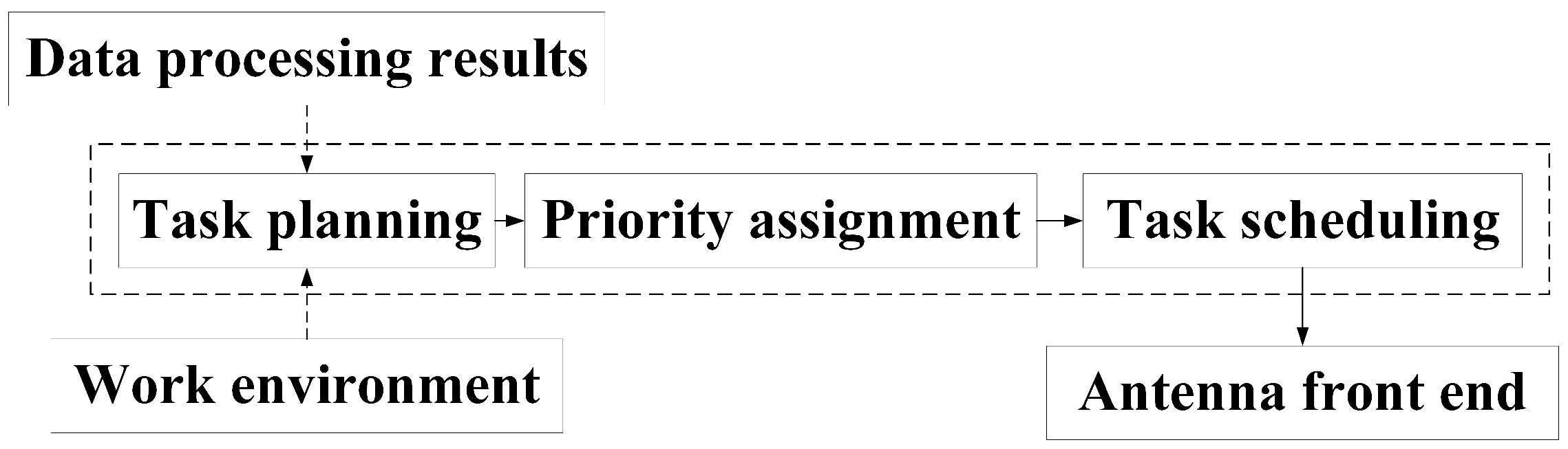
The resource scheduling function of phased array radar usually consists of three parts: “task planning”, “priority assignment”, and “task scheduling”, as shown in Figure 1.
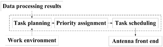
Figure 1.
Module composition of phased array radar resource scheduling system.
2.1. Task Planning Module
Task planning module focuses on the “task requests” generated via the phased array radar. Task requests specify the dwell type—such as search, confirmation, or tracking—and include relevant execution parameters, such as the direction of the transmitted beam, transmission power, expected execution time, and time window, etc. When planning dwell tasks, it is necessary to consider the working requirements of the radar, the working environment, and the filtering results of the data processing outputs.
2.2. Priority Assignment Module and Dwell Task Model
The priority assignment module computes the overall priority of each task through a weighted summation based on factors such as the importance of different task types and the threat level of tracking targets. Specifically, it considers a combination of each task’s execution deadline (reflecting task urgency), the inherent priority of its operation mode (e.g., confirmation tasks have higher mode priority than tracking tasks), and the threat level of the associated target. Currently, a common method for determining threat level is the analytic hierarchy process (AHP), which calculates threat scores by weighting parameters such as relative radial distance, velocity, angle, and altitude of the target, as illustrated in reference [19]. Alternatively, threat levels may also be provided via an external system. However, since threat level evaluation is treated as an external input to the scheduling algorithm and does not affect the timing design or complexity analysis of the scheduling model itself, this paper does not discuss the specific method for determining threat level in detail. After the priority assignment is completed, the task model input into the task scheduling module.
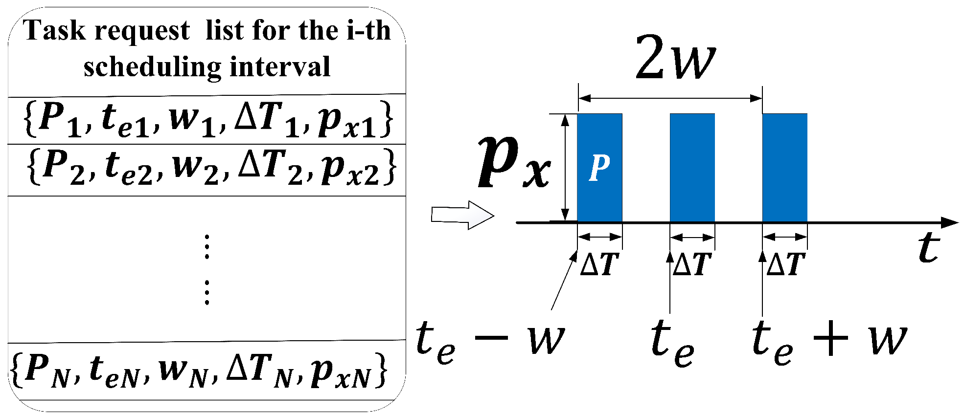
In (1), P denotes the task priority, is the expected execution time, w is the time window length, T is the dwell length, is the transmission power. When a task is executed, its actual execution time should satisfy the condition: − w ≤ ≤ + w. The actual execution time is determined by the scheduling results of the task scheduling module. The mapping relationship from the task request list to the actual dwell tasks is shown in Figure 2.
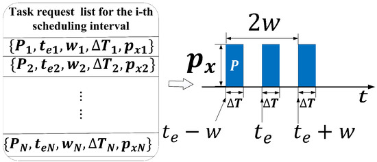
Figure 2.
The mapping relationship from the task request list to the actual dwell tasks. The left side of the figure represents the task request list, where each row corresponds to a task and contains its associated information, including priority, dwell time, and other parameters. The right side illustrates the mapping of this information onto the time axis. The time window w defines the allowable range within which a task can be executed relative to its expected execution time. Specifically, − w is the earliest possible execution time for the task, while + w is the latest permissible execution time (i.e., the deadline).
2.3. Task Scheduling Module
Based on the task information in the above task request list, actual execution times for each task are scheduled under the constraints of radar resources such as time and energy. This scheduling is accomplished by selecting appropriate task scheduling strategies, such as prioritizing high-priority tasks, maximizing task scheduling success rates, and minimizing task execution time shifts. The tasks in the request list are then categorized into an execution task queue, a delayed task queue, and a deletion task queue. The tasks in the execution task queue are sent to the antenna front-end for execution, tasks in the delayed task queue are temporarily retained, and tasks in the deletion task queue are dropped, thereby completing the resource scheduling process.
Considering the overall structure of the resource scheduling module described above, we observe that existing task scheduling strategies often face challenges when handling high-load and multi-type task scenarios under constrained radar resources. In particular, conventional scheduling approaches fail to make full use of the radar idle periods between transmission and reception phases and often lack effective mechanisms to control the deviation between actual and expected task execution times. These limitations motivate the design of a more refined scheduling method. In the following section, we introduce a novel scheduling method that integrates pulse interleaving with time-pointer-based scheduling, further enhanced via time shifting constraints, to improve scheduling efficiency and controllability under resource-constrained conditions.
3. The Scheduling Method Based on Time Shifting Constraints and Pulse Interleaving
3.1. Pulse Interleaving Technology
To further enhance the utilization of time resources, pulse interleaving technology is introduced. Pulse interleaving uses the wait interval of a task (during which the radar is idle) to execute the transmit and/or receive dwell of another task. For tracking tasks, the length of the task waiting period can be calculated based on the distance of the target. However, for search tasks, in the absence of prior information, it is not possible to calculate the waiting period between the transmission and reception of echoes due to the lack of distance information of the target. Therefore, pulse interleaving is not applicable to search tasks, which instead immediately enter the reception phase after transmission. Let the task request list based on pulse interleaving be T = [, ,…,], where represents the i-th task in the list T. The task model is defined as follows:
where , , and are denoted as the length of the transmit dwell time, the wait interval, and the receive dwell time, respectively. In general, the power consumed by receiving a signal is significantly less than the power consumed by transmitting a signal. Therefore, when considering energy constraints in this paper, we ignore the power consumption of receiving signals and only consider the power consumption of transmitting signals . The dwell task model based on pulse interleaving is shown in Figure 3.
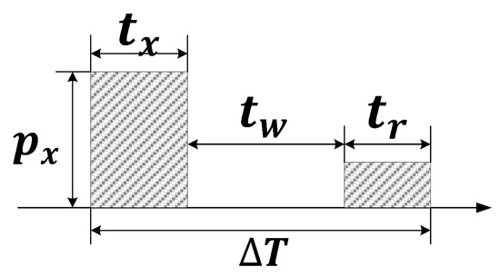
Figure 3.
Dwell task model based on pulse interleaving. The task is divided into transmit, wait, and receive phases, where only the transmit phase consumes power and is considered in the energy-constrained scheduling model.
Based on the model shown in Figure 3, two types of pulse interleaving methods are presented, as illustrated in Figure 4. Let the previously executed task be , and the currently executing task is .
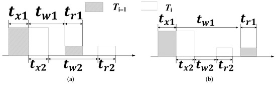
Figure 4.
Two types of pulse interleaving methods. (a) Partial interleaving. The transmission of task is initiated during the waiting period of task . After completes its reception phase, continues with its own waiting and reception phases. This interleaving approach allows tasks to share idle periods effectively. (b) Fully interleaving. The entire execution process of task (including transmission, wait, and reception) is fully embedded within the wait interval of the previous task . This requires that the dwell time of task must be shorter than the wait interval of .
As can be seen, there are two modes of pulse interleaving. One is that only the transmit interval of a task can be interleaved with the wait interval of another task, which is termed partial interleaving. The other is that the entire duration of a task can fit in the wait interval of another task, which is termed fully interleaving. Therefore, if two tasks are eligible for pulse interleaving, their transmission and reception periods must not overlap. The time constraints that must be met to implement the two types of pulse interleaving mentioned above are as follows:
For the mode in Figure 4a:
for the mode in Figure 4b:
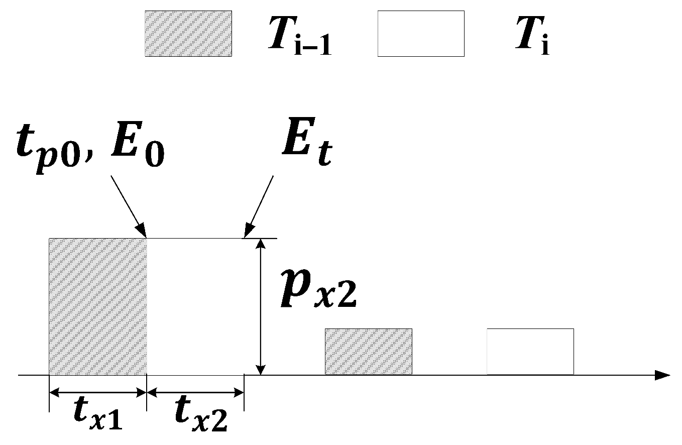
The task scheduling based on pulse interleaving increases the continuous operation time of the radar, leading to higher energy consumption and a rise in the system’s temperature. When the temperature rises beyond the limit range that the radar system can withstand, it can cause damage to the radar system. Therefore, energy constraints must also be considered, as shown in Figure 5. is the end time of the launch period for task , is the total energy consumption of the system at the end of task launch, and is the total energy consumption of the system at the end of task launch. If the energy consumption of the system at time is E and the radar does not perform any tasks in the following time, then at time + T, the system energy becomes the following:

Figure 5.
Energy constraints of pulse interleaving. is the system’s energy consumption at the end of the transmission period of , and is the system’s energy consumption after the transmission period of when executed in an interleaved manner. Therefore, to enable the interleaved execution of and , it is necessary to guarantee that the system’s energy consumption at the end of ’s transmission period remains below a predefined threshold.
In (5), is the look-back period, which characterizes the heat dissipation performance of the radar. If task is executed at time , the total energy consumption of the system at the end of the mission launch period is as follows:
Let be denoted as the endurable maximal instantaneous energy consumption; then, the energy constraint is expressed as follows:
In summary, two tasks can be interleaved only if they satisfy either (3) or (4), and also meet the energy constraint in (7), as illustrated in Figure 6.
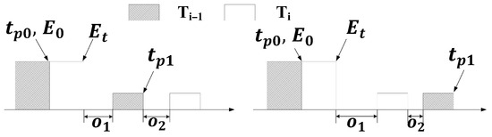
Figure 6.
Parameter updates for the pulse interleaving method. The left part of the figure represents the result after partial interleaving, while the right part shows the result after fully interleaving. denotes the time point at which the transmission of the task ends and serves as the baseline of the system’s energy state before interleaving. represents the time point at which the reception of the task ends. The interleaved execution of tasks cannot violate the system’s energy constraint, so the cumulative energy consumption between and must remain below the energy threshold.
When two tasks are successfully interleaved, two new idle periods, and , are created. To simplify the scheduling process, the two interleaved tasks are merged into a composite task, and is considered the wait interval for the new task. After forming the new task, its parameters are updated as follows:
- (1)
- If the interleaving method shown in Figure 4a is adopted, the parameters of the new task are updated as follows:
- when :
- when :
- (2)
- If the interleaving method shown in Figure 4b is adopted, the parameters of the new task are updated as follows:
- when :
- when :
3.2. The Description of Proposed Methodology
After combining the pulse interleaving method with the time pointer scheduling method, it is also necessary to consider the issue of large time shifting. This paper introduces a time shifting constraint mechanism by assigning a maximum allowable time-shift ratio to each task. A task can only be scheduled if its execution time shifting ratio meets this constraint. The constraints of the time shifting-constrained scheduling method, incorporating both the time-pointer and pulse interleaving methods, are as follows: represents the expected execution time of the i-th task; represents the time window length of this task; represents the start time of a given scheduling interval; represents the ending time of the scheduling interval; represents the actual execution time of the i-th task; , , and are the lengths of the transmit duration, wait interval, and receive duration, respectively; represents the number of tasks in the radar execution task queue; represents the total energy consumption of the radar system at time t; represents the threshold for total energy consumption of the system; represents the expected execution time of the k-th task in the deletion task queue, represents its time window length, and represents the number of tasks in the deletion queue.
Equation (16) states that the actual execution time of each task must be later than the maximum value of the earliest executable time and the start time of the scheduling interval, while the end time of the task must be earlier than the minimum value of the deadline of this task and the end time of the scheduling interval; Equation (17) is designed to prevent time conflicts between scheduled radar tasks. Equation (18) is the time shifting constraint condition, which enforces that a task can only be scheduled if its time shifting rate is below a preset threshold. In this equation, represents the threat degree of task i, and and are adjustable parameters used to modify the range of time shifting based on operational requirements or actual conditions. As the priority and threat degree of the target gradually increase, the upper limit of the time shifting for tracking task gradually decreases; Equation (19) represents the energy constraint condition, and Equation (20) is the condition for the task to be dropped. Based on the previous description, the overall flowchart of the algorithm is shown in Figure 7.
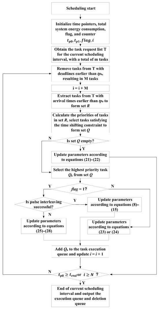
Figure 7.
Flowchart of scheduling algorithm.
We can summarize the whole processing flow of the method as follows:
- (1)
- Scheduling begins. Initializing the time pointers and to point to the start time of the scheduling interval, i.e., = = ; Initialize counter i = 0, system energy , and pulse interleaving identifier . The variable ∈{0,1} is a binary decision variable that takes on the value 1(0) if the current task can be interleaved with the previous task (cannot be interleaved).
- (2)
- Let the task request list within the scheduling interval [,] be denoted as T = [,,…,].
- (3)
- All tasks in T that satisfy the condition + w < are moved to the deletion list. Let the total number of such tasks be M, and update the counter by setting i = i + M.
- (4)
- Find all tasks from T that satisfy + w < , which can be executed at time , to form a task set R = [,,…,], and calculate the priority of tasks in R. The method for calculating priority follows an improved MHPF (Modified Highest Priority First) criterion: Let the work mode priority of each task in set R be denoted as P = [,,…,], the deadlines as = [,,…,], and the threat degrees as = [, ,…, ]. Task i is considered to have a higher priority than task j if > , or if = , > , or if = , = , < .
- (5)
- Select all tasks from the set R that satisfy the shifting constraint given in (18) to form a new set Q = [,,…,]. If Q is empty, meaning that none of the tasks in Q satisfy the shifting constraints of (18), proceed to Step 6; otherwise, proceed to Step 7.
- (6)
- Update time pointers , , and total system energy consumption:when = :otherwise:where l represents the minimum step length for the time pointer to slide; proceed to Step 8.
- (7)
- Find the task with the highest priority from set Q:
- (a)
- If = 0, it indicates that task cannot be interleaved with the previous task. In this case, schedule task at time and move into the execution task queue. If task can be interleaved, then update parameters according to (23); if interleaving is not possible, then update parameters and tp1 according to (24). Based on the type of task , update and , and increment i by 1.
- (b)
- If = 1 and task satisfies the constraints of (3), (4), (7), and (17), then task is moved into the execution task queue, i is incremented by 1, and the parameters are updated according to (8) to (15). If task does not satisfy the constraints, the parameters are updated according to (25) to (28).when , the following applies:In other cases:
- (8)
- Check whether or . If either condition is true, the task scheduling for the current interval is complete. Delete the time pointers, and output the execution queue and deletion queue for this scheduling interval. Otherwise, proceed to Step 3.
The proposed scheduling algorithm primarily involves task interleaving determination and time-shifting arrangement. In each scheduling window, only the currently ready task set (denoted as q) is considered. Among them, a subset of tasks (typically tracking tasks, denoted as n) require interleaving conflict checking. For each such task, the algorithm checks all other overlapping tasks to determine temporal compatibility, resulting in an interleaving complexity of per cycle. Additionally, priority assignment and feasible interval extraction are conducted before interleaving. The priority computation is , while the interval check is bounded and does not scale with q or the total number of tasks, N. As a result, the per-cycle complexity is dominated by the term.
Assuming the number of scheduling cycles is T, the total worst-case complexity becomes . In practice, the number of tracking tasks, n, is typically much smaller than N, and the number of ready tasks, q, is also constrained due to radar resource limits. Furthermore, the use of the time pointer and shifting constraints helps prune infeasible options early, reducing unnecessary comparisons. Therefore, the algorithm achieves good real-time performance and is well suited for deployment in resource-constrained radar-scheduling scenarios.
With the above model and optimization formulation in place, we now proceed to evaluate the proposed algorithm through simulation experiments under representative radar scenarios.
4. Simulation and Results
To validate the effectiveness of the proposed scheduling method, a series of simulation experiments are conducted under various task scenarios. These experiments are designed to evaluate the proposed method’s performance in terms of the scheduling success rate, execution efficiency, priority assurance, and time shifting control. Both the traditional time-pointer-based method and the improved approach are tested for comparison.
4.1. Scheduling Performance Evaluation Metrics
To validate the effectiveness of the proposed method, the following evaluation metrics are employed for performance assessment:
- (1)
- Scheduling Success Ratio (SSR):represents the number of successfully scheduled tasks, and N denotes the total number of radar tasks requested to be scheduled. The SSR is defined as the proportion of successfully scheduled tasks.
- (2)
- Average time shift ratio (ASTR):represents the time window length of task i, is the expected execution time of task i, and is the actual execution time of task i. The ATSR indicates the timeliness of task scheduling.
- (3)
- Hit value ratio (HVR):represents the number of successfully scheduled tasks, denotes the priority of each successfully scheduled task, N is the total number of radar tasks requested for scheduling, and represents the priority of all tasks requested for scheduling. HVR quantifies the proportion of radar resources (such as time and energy) that successfully contribute to the high-value tasks such as detection, tracking, and engagement of targets.
4.2. Scenario and Parameter Settings
The simulation parameters are listed in Table 1. The scheduling interval is 50 ms, and the simulation time is 5 s. The simulation includes four typical types of phased array radar tasks: confirmation, precision tracking, general tracking, and airspace search. Confirmation tasks are triggered immediately upon target detection, and each target requires only a single confirmation instance. The expected execution times are uniformly and randomly distributed within the interval [0, 4 s]. The tracking task for each target is generated at a fixed data rate after the confirmation task is completed. The ratio of the number of targets tracked normally to those tracked precisely is 2:1. The threat degrees of precise tracked targets and general tracked targets are uniformly and randomly distributed within (0.5, 1] and (0, 0.5], respectively. The number of targets ranges from 12 to 108, with the experiment repeated 100 times for each increment of 12 targets, and the results are averaged. = 0.5, = −1; l = 1 ms, = 250 J, and = 150 ms.

Table 1.
Simulation task parameters.
4.3. Simulation Results
For clarity, the time-pointer scheduling method is referred to as the “traditional method,” while the proposed approach is termed the “improved method.”
The simulation results are shown in Table 2 and Table 3 and Figure 8 and Figure 9. Table 2 and Table 3 summarize the results for the traditional method and the proposed method, respectively. Each table reports the mean ± standard deviation of various evaluation metrics across 100 simulation runs under different numbers of targets. Figure 8 illustrates the trends of these metrics as the number of targets increases, while Figure 9 depicts the variation in the time shift ratio corresponding to targets with different threat levels.
Table 2.
Scheduling performance metrics (mean ± std) under different numbers of targets using the traditional method.
Table 3.
Scheduling performance metrics (mean ± std) under different numbers of targets using the proposed method.
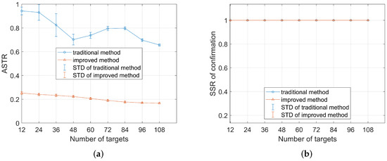
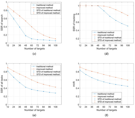
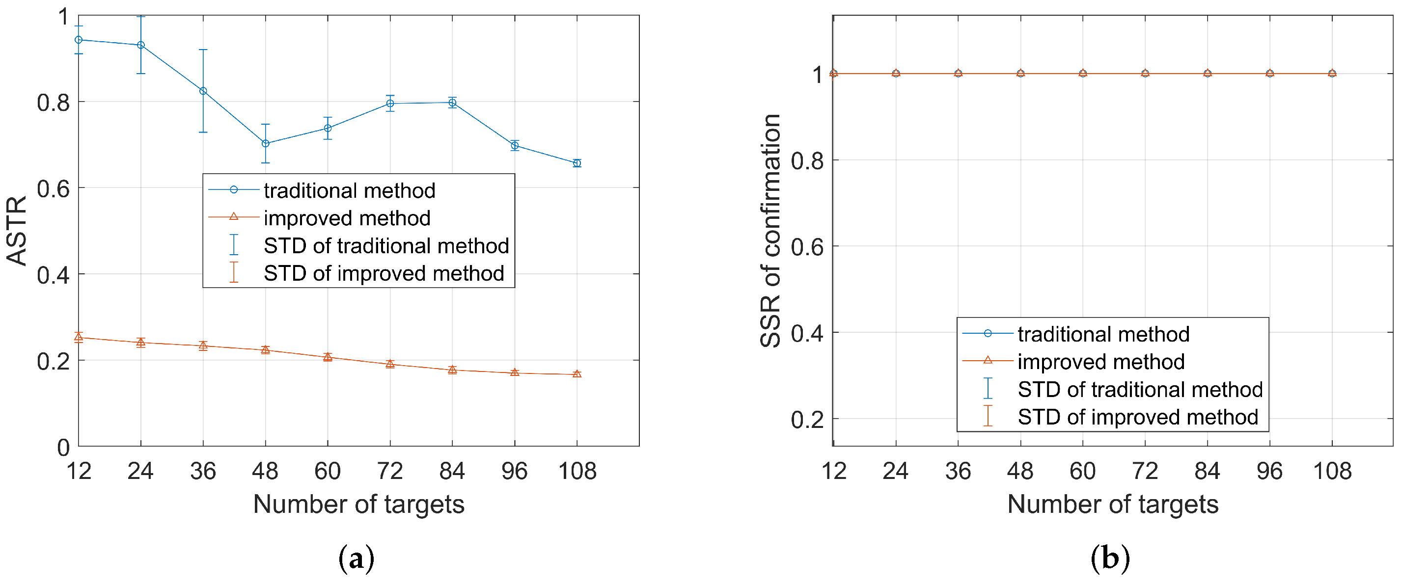
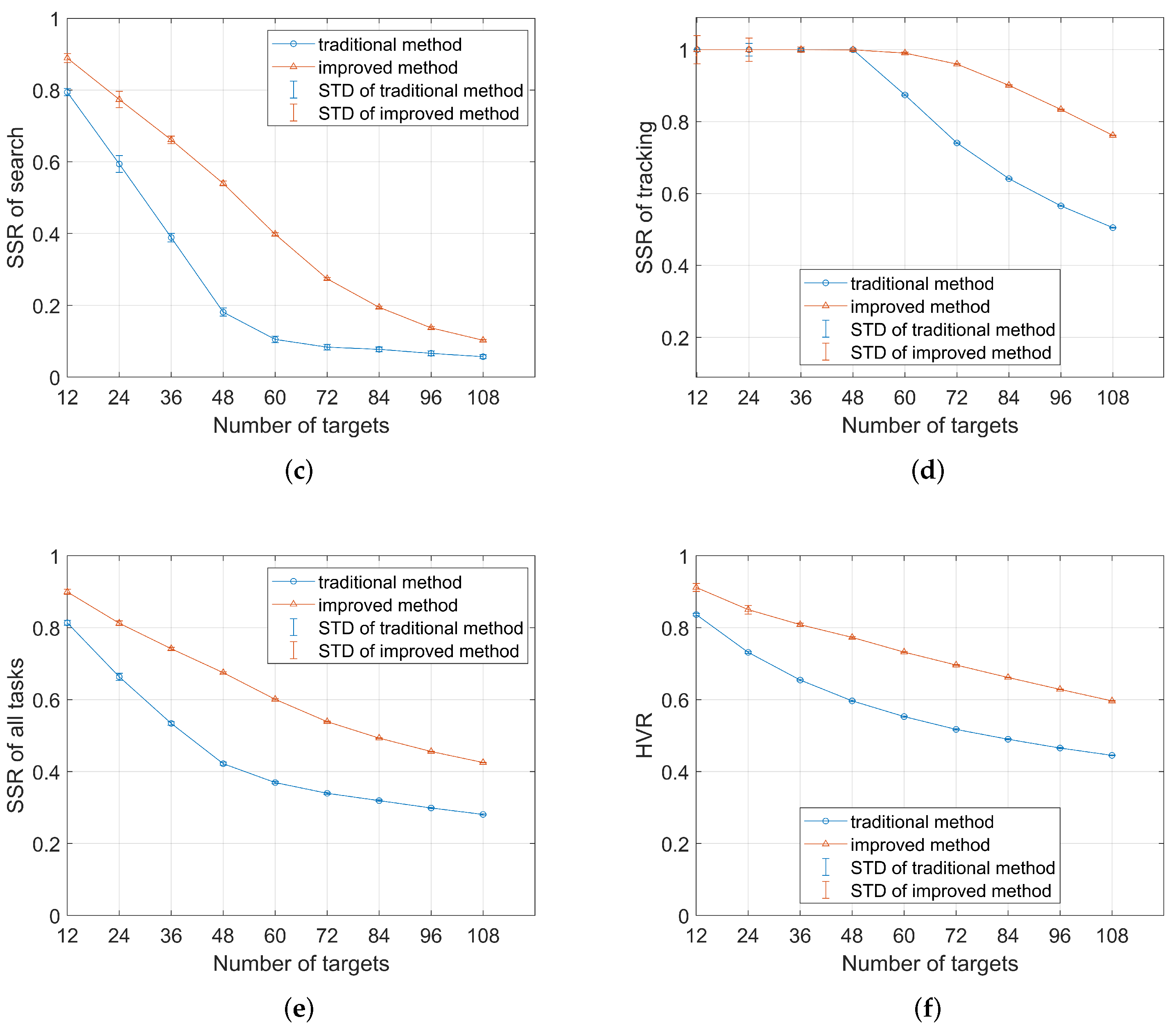
Figure 8.
Experimental results of task scheduling using the traditional time-pointer method and the proposed improved method. The orange curve represents the improved method, while the blue curve represents the traditional method. The error bars on the curves indicate the standard deviation obtained from 100 simulations for each target quantity. The figure contains the following subplots. (a) Average time shifting ratio. (b–d) Scheduling success rates for confirmation, search, and tracking tasks, respectively. (e) The proportion of successfully scheduled tasks among all requested tasks. (f) The proportion of high-priority tasks among the executed tasks.
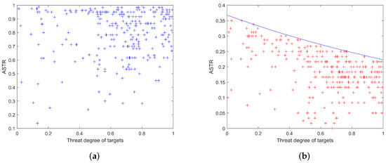
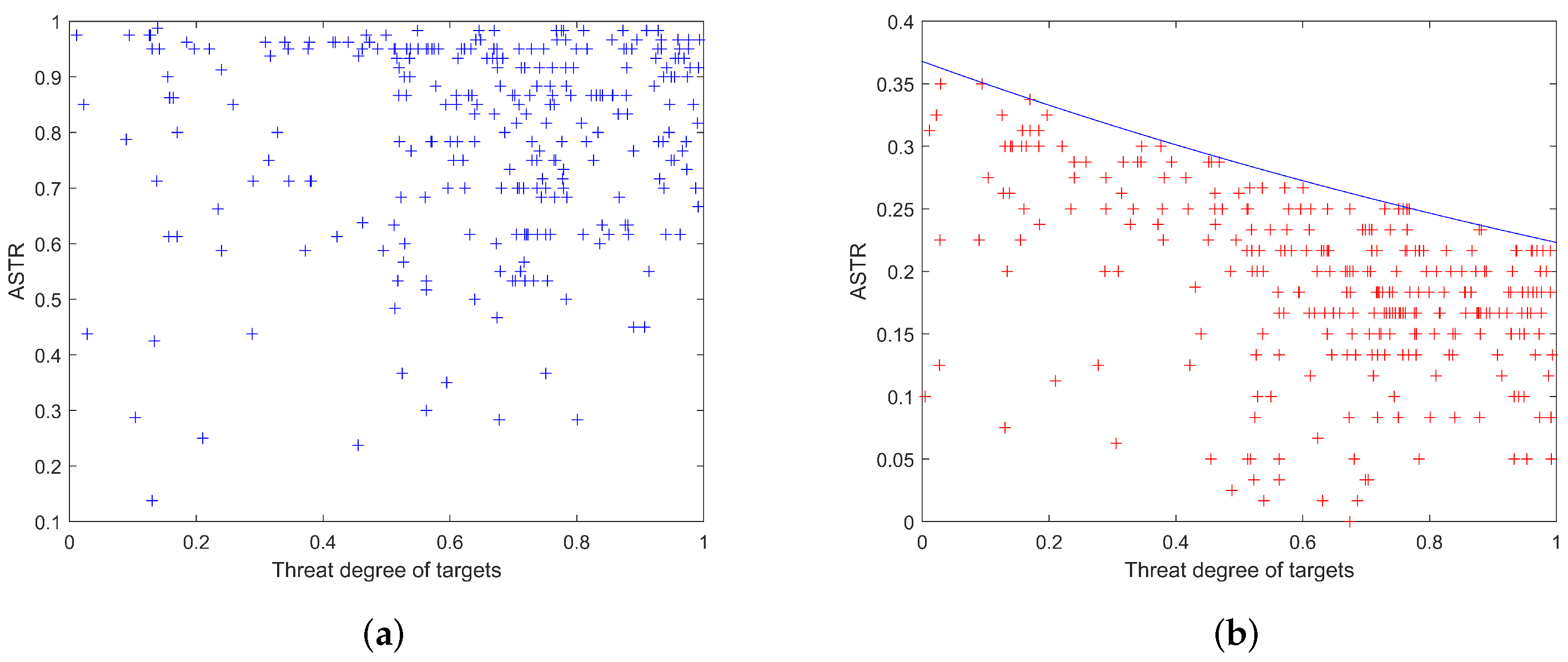
Figure 9.
ASTR of targets with different threat degrees. (a,b) respectively show the average time shifting ratios of targets with different threat levels after scheduling using the traditional method and the improved method. In (b), the blue curve represents the upper bound of the time shifting ratio corresponding to targets of different threat levels.
Figure 8a compares the average time shift ratios between the traditional and improved methods. It is evident that, regardless of the number of targets, the average time shift ratio of the improved method is significantly lower than that of the traditional method. This is because the improved method imposes constraints during the scheduling of each task, strictly controlling the time shifting range for each task. Specifically, the traditional method allows task execution at any point within the permissible window between the earliest start time and the deadline. However, with the time shifting constraint applied in the improved method, the execution time of tasks is confined within a range that achieves timely execution. Compared to low-threat, low-speed, and low-maneuverability targets, the tracking accuracy of high-threat, high-speed, and high-maneuverability targets is more significantly affected by time shifting. Additionally, the tasks associated with high-threat targets are often of greater importance. Therefore, the execution time of high threat targets needs to be closer to the expected execution time.
From the simulation perspective, since each target quantity configuration was independently simulated 100 times, the standard deviation of ASTR is relatively higher when the number of targets is small. In this case, the scheduling system has more flexibility, leading to greater variation in task execution order and resource allocation across different simulations. As the number of targets increases, the scheduling becomes more compact and constrained, reducing the differences between simulation results and thus lowering the standard deviation of ASTR.
Figure 9 presents the time shift ratio for the execution of tasks associated with targets of different threat degrees. The blue and red “+” symbols in the figure represent the time-shifting ratio corresponding to tracking tasks with different threat levels, scheduled by the traditional method and the improved method, respectively. The horizontal axis represents the target threat degree, and the vertical axis represents the time shift ratio. In Figure 9b, the blue curve denotes the upper limit of time shift ratios for targets with varying threat levels, which corresponds to the time shifting threshold for targets of different threat degrees.
As shown in Figure 9a, the traditional methods only consider the utilization of time resources during scheduling, without taking into account the situation of time shifting, resulting in a high time shift ratio for most of the scheduled tasks; In contrast, Figure 9b demonstrates that as the target threat degree increases, the maximum deviation between the actual and expected execution times of tasks gradually decreases. The time shift ratio of targets with different threat degrees is within the control range, making the actual execution time of high threat targets as close as possible to the expected execution time. Additionally, parameters and can be adjusted according to specific work requirements or target tracking situations, thereby adjusting the upper limit of time shifting for tasks with different degrees of threat.
Figure 8b,d show the variation in the schedule success ratios of different task types as the number of targets increases, after being scheduled by the two methods. First, both methods consistently prioritize high-priority tasks, including confirmation and precise tracking. In addition, the improved method demonstrates higher scheduling success ratios for both search tasks and tracking tasks compared to the traditional method. This is attributed to the introduction of pulse interleaving in the improved method, thereby making more efficient use of the system’s idle time resources and enhancing the overall schedule success ratio. Figure 8e,f illustrate that the total task schedule success ratio and hit value ratio for both methods decrease as the number of targets increases, with the improved method consistently outperforming the traditional method.
The simulation results also reveal that, when the number of targets is large, the traditional method allocates most of the resources to higher-priority tasks such as confirmation and tracking, leaving fewer resources for search tasks. However, with the improved method, tracking tasks can be interleaved with other types of tasks. As a result, executing the same number of tracking tasks with the improved method requires less time, and then the saved time and resources can be used to perform other types of tasks such as search tasks. Overall, compared to traditional methods, the improved approach achieves more efficient resource allocation and enhances overall radar performance.
5. Discussion and Concluding Remarks
To enhance the on-orbit safety of manned spacecraft and avoid the threat of constellations, it is necessary to consider equipping them with phased array radar systems for large-scale search and tracking in the future. However, traditional scheduling methods for phased array radar have low scheduling efficiency when facing task requests generated via a large number of satellites and space debris. To enhance the resource allocation capability and efficiency of space station protection radar, this paper investigates adaptive scheduling methods. This paper analyzes the time pointer task scheduling method and proposes a scheduling method based on time shifting constraints and pulse interleaving to address the problems of a large average time shift ratio and idle task waiting period in this method. By interleaving radar tasks using pulse interleaving technology, the proposed method makes more efficient use of time resources and effectively reduces task execution time shifting through shifting constraints. In conclusion, simulation experiments demonstrate that the method proposed in this paper effectively reduces the average time shift ratio while significantly improving task scheduling success ratios and other performance metrics. Consequently, the space station protection radar achieves superior performance when confronted with a large number of targets requiring tracking and monitoring.
Author Contributions
Conceptualization, G.Z. and H.Y.; methodology, G.Z. and H.Z.; software, G.Z. and J.H.; validation, G.Z. and G.X.; formal analysis, G.Z. and H.Z.; investigation, J.H. and G.X.; resources, G.Z.; data curation, G.X.; writing—original draft preparation, G.Z. and D.W.; writing—review and editing, G.Z. and D.W.; visualization, H.Z.; supervision, H.Y. All authors have read and agreed to the published version of the manuscript.
Funding
This research received no external funding.
Data Availability Statement
No new data were created or analyzed in this study.
Conflicts of Interest
The authors declare no conflicts of interest.
References
- McDowell, J.C. The low earth orbit satellite population and impacts of the SpaceX Starlink constellation. Astrophys. J. Lett. 2020, 892, L36. [Google Scholar] [CrossRef]
- Muntoni, G.; Montisci, G.; Pisanu, T.; Andronico, P.; Valente, G. Crowded space: A review on radar measurements for space debris monitoring and tracking. Appl. Sci. 2021, 11, 1364. [Google Scholar] [CrossRef]
- Dobritsa, D.; Pashkov, S.; Khristenko, I.F. Protective properties of pleated wire mesh shields for spacecraft protection against meteoroids and space debris. In AIP Conference Proceedings; AIP Publishing: Melville, NY, USA, 2021; Volume 2318. [Google Scholar] [CrossRef]
- Buchs, R.; Florin, M.V. Collision Risk from Space Debris: Current Status, Challenges and Response Strategies. 2021. Available online: https://infoscience.epfl.ch/handle/20.500.14299/178442 (accessed on 6 January 2025).
- Murtaza, A.; Pirzada, S.J.H.; Xu, T.; Jianwei, L. Orbital debris threat for space sustainability and way forward. IEEE Access 2020, 8, 61000–61019. [Google Scholar] [CrossRef]
- Kollias, P.; Palmer, R.; Bodine, D.; Adachi, T.; Bluestein, H.; Cho, J.Y.; Griffin, C.; Houser, J.; Kirstetter, P.E.; Kumjian, M.R.; et al. Science applications of phased array radars. Bull. Am. Meteorol. Soc. 2022, 103, E2370–E2390. [Google Scholar] [CrossRef]
- Yang, J.; Lu, X.; Dai, Z.; Yu, W.; Tan, K. A cylindrical phased array radar system for uav detection. In Proceedings of the 2021 6th International Conference on Intelligent Computing and Signal Processing (ICSP), Xi’an, China, 9–11 April 2021; pp. 894–898. [Google Scholar] [CrossRef]
- Basha, M.; Ware, N.R. Design for Reliability of Phased Array Radars. In Proceedings of the 2021 6th International Conference for Convergence in Technology (I2CT), Maharashtra, India, 2–4 April 2021; pp. 1–5. [Google Scholar] [CrossRef]
- Gao, T.; Wei, Q.; Wang, P.; Dong, Y.; Jiang, H.; Zhu, B. The development status and trend of airborne multifunctional radar. In Proceedings of the 2021 IEEE International Conference on Artificial Intelligence and Industrial Design (AIID), Guangzhou, China, 28–30 May 2021; pp. 327–330. [Google Scholar] [CrossRef]
- Han, Q.; Zhang, Y.; Yang, Z.; Long, W.; Liang, Z. Antenna array aperture resource management of opportunistic array radar for multiple target tracking. IEEE Access 2020, 8, 228357–228368. [Google Scholar] [CrossRef]
- Cheng, T.; Liu, L.; Li, Z.; Heng, S. Real-Time Dwell Scheduling Based on a Unified Pulse Interleaving Framework for Phased Array Radar. Tsinghua Sci. Technol. 2024, 29, 1540–1553. [Google Scholar] [CrossRef]
- Li, B.; Tian, L.; Chen, D.; Han, Y. A task scheduling algorithm for phased-array radar based on dynamic three-way decision. Sensors 2019, 20, 153. [Google Scholar] [CrossRef]
- Meng, F.; Tian, K. Phased-array radar task scheduling method for hypersonic-glide vehicles. IEEE Access 2020, 8, 221288–221298. [Google Scholar] [CrossRef]
- Zhang, H.; Xie, J.; Ge, J.; Zhang, Z.; Zong, B. A hybrid adaptively genetic algorithm for task scheduling problem in the phased array radar. Eur. J. Oper. Res. 2019, 272, 868–878. [Google Scholar] [CrossRef]
- Li, Z.; Cheng, T.; Heng, S. Real-time dwell scheduling algorithm for phased array radar based on a backtracking strategy. IET Radar Sonar Navig. 2023, 17, 261–276. [Google Scholar] [CrossRef]
- Luo, M.; Jiang, B.; Xing, W.g. Networked Radar Mission Planning Algorithm Based on Pulse Interleaving and Cross-Scheduling Interval. J. Phys. Conf. Ser. 2023, 2670, 012027. [Google Scholar] [CrossRef]
- Duan, Y.; Tan, X.S.; Qu, Z.G.; Wang, H. Index for task scheduling in phased array radar. J. Eng. 2019, 2019, 7550–7554. [Google Scholar] [CrossRef]
- Hao, L.; Yang, X.; Hu, S. Task scheduling of improved time shifting based on genetic algorithm for phased array radar. In Proceedings of the 2016 IEEE 13th International Conference on Signal Processing (ICSP), Chengdu, China, 6–10 November 2016; pp. 1655–1660. [Google Scholar] [CrossRef]
- Luo, R.; Huang, S.; Zhao, Y.; Song, Y. Threat Assessment Method of Low Altitude Slow Small (LSS) Targets Based on Information Entropy and AHP. Entropy 2021, 23, 1292. [Google Scholar] [CrossRef]


Disclaimer/Publisher’s Note: The statements, opinions and data contained in all publications are solely those of the individual author(s) and contributor(s) and not of MDPI and/or the editor(s). MDPI and/or the editor(s) disclaim responsibility for any injury to people or property resulting from any ideas, methods, instructions or products referred to in the content. |
© 2025 by the authors. Licensee MDPI, Basel, Switzerland. This article is an open access article distributed under the terms and conditions of the Creative Commons Attribution (CC BY) license (https://creativecommons.org/licenses/by/4.0/).