Article

Detection of Transmission State of Multiple Wireless Sources: A Statistical Mechanics Approach

by
Spyridon Evangelatos
1,2,* and
Aris L. Moustakas
1
1
Department of Physics, National and Kapodistrian University of Athens, Zografou, 15710 Athens, Greece
2
Netcompany-Intrasoft S.A., 2b, rue Nicolas Bové, L-1253 Luxembourg, Luxembourg
*
Author to whom correspondence should be addressed.
Telecom 2023, 4(3), 649-677; https://doi.org/10.3390/telecom4030029
Submission received: 26 June 2023 / Revised: 14 July 2023 / Accepted: 4 September 2023 / Published: 18 September 2023

Abstract

:
Consider a random network of static primary wireless sources and a co-located network of secondary wireless devices. The channel coefficients between the two networks are assumed to be known to the secondary users (SUs), e.g., using radio environment maps (REM). However, the operational state of the sources is unknown due to intermittency. In this paper, we study the performance of primary source detection by SUs using a message-passing algorithm. Additionally, we employ methods from statistical mechanics, in particular, the Replica approach, to obtain analytic results for the performance of such networks in the large system-size limit. We test the results through a large-scale simulation analysis, obtaining good agreement. The proposed method provides a simple way to evaluate the performance of the system and assess how it depends on the macroscopic parameters that characterize it, such as the average density of SUs and sources and the signal-to-noise ratio. The main contribution of this paper is the application of an algorithm that quantitatively predicts the parameter value region for which accurate and reliable detection of the operational state of the primary sources can be achieved in a fast and decentralized manner.

1. Introduction

Dynamic spectrum sensing has emerged as an important approach to deal with spectrum scarcity, which is caused by the deployment of many IoT-enabled devices [1], where secondary users/devices monitor a given spectrum band to determine the presence (or absence) of active (licensed) sources, whose state is dynamic and intermittent in time. This method guarantees that subsequent usage of the spectrum by secondary opportunistic users does not result in significant interference with the primary source communications and vice versa. The above is a particular paradigm of a Cognitive Radio (CR)-enabled IoT network [2], which injects high-level intelligence into IoT networks and assists sensor nodes in using the available spectrum without interfering with the primary sources. In addition, it improves the whole system throughput compared to traditional homogeneous network topologies [3] (i.e., classical cellular, ad hoc), and as a promising enabler communication technology for the IoT, it attains the levels of performance and efficiency required by future wireless communications.
The identification of emitting sensors in the context of a Cognitive Radio-enabled IoT network is of paramount importance. Apart from the enhanced spectrum efficiency, where the identification of emitting sources can assist in efficiently utilizing the available spectrum by avoiding interference and allocating frequency bands to different IoT devices, it improves the coexistence and compatibility of various devices and systems in the same environment, such as Wi-Fi, Bluetooth, Zigbee, and other wireless technologies [4]. Thus, identifying the emitting sources allows Cognitive Radio systems to determine which devices are using which frequencies or channels, enabling them to select available and interference-free channels for their own communication. From a network security perspective, the identification of emitting sources also allows for the detection of unauthorized or malicious devices in the network, revealing potential security threats or unauthorized access points [5]. Last, by identifying the emitting sources, network operators can gain insights into the utilization of the radio spectrum. This information can be used for network planning, optimization, and resource management and assist network operators in designing efficient IoT deployments, identifying areas of congestion, and improving the overall network performance.
In a Cognitive Radio-enabled IoT network deployment in a smart home environment, such as the one depicted in Figure 1 the primary sources can be the devices or systems designed to send data or information within the network. These devices can be Wi-Fi Access Points, which provide wireless connectivity within the smart home network and act as primary sources of radio signals for data transmission. Zigbee or Z-Wave hubs are also systems that are commonly used for smart home automation and control, communicating with various Zigbee or Z-Wave devices such as smart lights, thermostats, door locks, etc. Bluetooth-enabled devices, such as smartphones, smart speakers, wearables, etc., are also included in the long list of devices within a smart home network. On the other hand, secondary sources can potentially include wireless security cameras or surveillance systems, which may operate in frequency bands that overlap with Wi-Fi or other IoT protocols, leading to interference.
The detection and localization of primary sources can be accomplished by taking advantage of radio environment maps (REM) [6]. REMs are integrated databases that provide multi-domain environmental information regarding all devices that are capable of transmitting and/or receiving radio signals. The location information and power levels of primary sources are typical examples of stored information. However, since the state of these sources is intermittent and typically changes without notice at different times of the day, it is important to come up with algorithms that are able to periodically update the transmission states of the sources. One of the simplest and most robust methods is the use of non-coherent energy detection [7], which, compared to, e.g., time-of-arrival techniques, has low complexity and does not heavily depend on the presence of multiple reflections inside the propagation medium.
A number of previous works have studied the detection problem. More specifically, [8] focused on fixed architectures with feedback from a fusion center over limited bandwidth channels, which undergo multiple scattering and noise, and [9] focused on finite-sized networks with a specific graph structure. In both cases, a global fusion center is assumed, to which each SU transmits a function of its observation over a noisy channel. The existence of a fusion center becomes problematic when the network becomes large, especially when it varies with time. In this case, SUs need to dynamically update their information in a distributed fashion, indicating the necessity of distributed detection algorithms.
There are several algorithms that belong to the class of Bayesian inference algorithms and are known as message-passing algorithms [10], which, along with their variations [11,12,13], have been proven to be near-optimal in many optimization and inference problems. These algorithms constitute an appealing distributed computational scheme, which takes advantage of their local structure, by conveying iterative messages along the edges of a factor graph, with each message being updated by the messages coming in from the adjacent nodes. This message update process allows for parallelization and local updating [14,15] since it decomposes the optimization problem into smaller parts that can then be solved independently. However, the performance of the message-passing algorithms is network-specific since they require knowledge of the graph’s connectivity structure. Convergence speed is essentially sublinear with respect to the number of sources. Only two conditions are necessary for successful convergence, i.e., the sparsity [16] of the connectivity matrix and the presence of a local tree-like structure that prevents loops, where the algorithm typically stalls. It has mostly seen applications using binary states, in this case, corresponding to whether the sources are active emitters. For such systems, the convergence to the optimal threshold is almost always guaranteed for both random fully connected [17,18] and sparse (Erdős–Rényi-like) random graphical models. Such algorithms have also been applied to more general alphabets [19] in the case of non-sparse, fully connected graphs in the context of compressed sensing, where they have been shown to converge in the case of random graphs represented by full matrices [20,21] with only a few further assumptions.
In this paper, we apply the idea of message passing to the detection of the operational state of a network of primary sources in the presence of secondary users. In contrast to other approaches that focus on situations with a few primary and secondary sources, we are particularly interested in cases where these become large. Hence, our approach is not limited by the size of the network. We assume that the locations of the primary sources are known through radio neighborhood maps. Due to the multiple interferences that any given SU receives from multiple primary sources in its vicinity, it is not at all obvious how to robustly detect which primary sources present are operational. As demonstrated in this paper in Section 7, myopic approaches using a single SU to detect the state of a source in the presence of others fail spectacularly. Our main contribution in this paper is to analyze and quantitatively predict, for a given environment, the appropriate system’s parameter space, such as the node density and signal-to-noise ratio ( SNR ), where reliable detection of emitting sources can be achieved.
To achieve the above goal, we apply ideas from the physics of random media, obtaining self-consistent equations, which we then solve using the so-called population dynamics methodology. This allows us to calculate the probability of detection of the operational state of the primary sources in the presence of Rayleigh fading channels using a set of equations that corresponds to the so-called replica symmetric ansatz [22]. While this approach is known to work only in the case of random graphs without loops, we show that our results, obtained in two-dimensional, loopy graphs, are in good agreement with those for random Erdos–Renyi graphs [23]. This application of statistical mechanics in the context of wireless networks represents an innovative approach to analyzing and understanding the system’s behavior. The extensive simulations performed (described in Section 6) allow for a comprehensive assessment of our method’s performance and provide valuable insights into its effectiveness, verifying its accuracy, scalability, and computational complexity.
The above-mentioned replica method from physics allows us to obtain results for large-scale systems and estimate the theoretical limits for successful multi-source detection. As a result, our proposed method does not depend on the specific network structure, and one can easily obtain the error detection rate of an arbitrary network given the distributions of the density connections between primary sources and secondary users. For completeness, in Appendix A, we provide a concrete example of how this algorithm can be used in a distributed fashion.
In Table 1, a brief comparison of the proposed framework with various state-of-the-art methods is presented, accompanied by the relevant advantages and drawbacks of each method. In conclusion, our method seems superior since it combines high levels of accuracy, computational complexity, robustness to noise, and scalability. The utilization of BP allows for efficient message passing and inference, enabling more reliable and precise primary source detection compared to alternative techniques. Our method also offers additional advantages such as adaptability to various network topologies and flexibility in incorporating prior knowledge. These features set our proposed approach apart and position it as a reliable and accurate solution for the detection of emitting sources in wireless sensor networks.
The remainder of this paper is organized as follows. The system model is presented in Section 2, whereas Section 4 describes the connection to the statistical mechanics framework. Section 3 introduces the basic tools used in this paper, namely the belief propagation algorithm, which is then applied to detect the operational state of multiple primary sources. Section 5 introduces the replica symmetric solution for the particular model. In Section 6, the results obtained from numerical simulations are discussed. In Section 7, we introduce the idea of single-source detection through a myopic secondary user. We conclude this paper in Section 8 with a summary and plans for future work.

2. System Model

Let us consider a network comprising primary wireless source nodes and SUs, which are randomly placed in a certain region of area A , with the corresponding node densities denoted by n s and n t , respectively. The channel power gain at the location of the i-th SU due to the ν -th source is denoted by H i ν . Each source ν in the network is assumed to be in one of two states: idle, in which case its transmitting power π ν is zero, or active, with its transmitting power π ν > 0 . For simplicity, we assume that π ν is the same for all sources. Both H i ν and π ν are assumed to be known to the SUs through a REM entity. The received power at SU i is denoted by P i , which is a linear combination of the transmitted powers of all the primary sources in its neighborhood and can be expressed as
P i = ν = 1 N H i ν π ν 1 s ν 2
where s ν { 1 , + 1 } is a random variable that describes the emitting state of the ν -th primary source. It is convenient to define a shifted version of P i as
y i = P i 1 2 ν = 1 N H i ν π ν ν = 1 N G i ν s ν
where G i ν = H i ν π ν 2 . To model the effects of path loss and fading, we express G i ν as [35]
G i ν = p x i ν z i ν d i ν γ
where p = P ref π ν 2 , P ref is the reference power (in dBm) at a reference distance from the source node [36], z i ν is the shadow fading coefficient, x i ν is the fast fading component, d i ν is the Euclidean distance between the source ν and the i-th SU, and γ is the path loss exponent. The above-mentioned simple transformation, from π ν s ν , is widely used in various problems connected with statistical mechanics [37] and can be seen in Table 2.
For simplicity, we assume, as in [38], a simple thresholding approach, where an SU detects a source if
G i ν G 0
where G 0 depends on the sensitivity of an SU’s receiver and its minimum received energy. We then assume that all G i ν that do not satisfy this inequality vanish. We then neglect all other interferences since they are weak.
Thus, we can calculate the distribution of the number of SUs connected to a source and, correspondingly, the distribution of the number of sources connected to a single SU. Starting with the former case, we first note that due to the independence of the positions of the SUs, the probability P k of k SUs connected to a given source follows the Poisson distribution, i.e.,
P k = R k k ! exp R
where R = n s A eff , and A eff is the effective area where the SU is connected to a source in the presence of fading and shadowing, i.e., when G > G 0 , which is given by
A eff = 0 + d r 2 π r + d t 2 π exp t 2 2 × 0 + d x exp [ x ] Θ p x exp [ σ t ] r γ G 0 = π p G 0 2 γ Γ 2 γ + 1 exp 2 γ 1 σ 2 γ
where Γ ( · ) is the Euler Γ -function and Θ ( · ) is the step function. Similarly, the number of sources connected to a given SU follows the Poisson distribution, with the parameter T = n t A eff .
We can also evaluate the distribution of G for the connected sites as the normalized area density, such that G = r γ p x exp [ σ t ] > G 0 , which can be shown to be
P ( G | G > G 0 ) = 2 γ G 0 2 γ G 2 γ + 1
After the introduction of the channel model, we now describe the detection process. Define s = [ s 1 , s 2 , , s N ] T as a vector of length N, with s τ = ± 1 , depending on the operational state of the corresponding source, i.e., whether the source is on or off. We also assume that noise η i is added to the received signal at each secondary user, thus corrupting the signal. The form of the measurement vector at the i-th SU is then expressed by the following equation
y i = ν N ( i ) G i ν s ν + η i
where N ( i ) signifies the sources connected with secondary user i, i.e., those for which G i ν > 0 , and similarly, N ( ν ) is defined as the neighborhood of source ν .
Although the sparsity of the channel matrix G is obvious due to finite connectivity, which is a consequence of (4), we also make the assumption that the corresponding graph does not have short loops. Nevertheless, the embedding of the graph on a two-dimensional surface inevitably invalidates this assumption. As will be seen later on, the results obtained justify this assumption in accordance with [39]. The desired state vector of the system, s , can then be obtained by solving the following least-squares (LS) optimization problem
s ^ = argmin s { 1 , + 1 } N y G s 2
It is interesting to note that if η i is additive white Gaussian noise (AWGN), then the LS detection problem is identical to the maximum a posteriori (MAP) estimate, in which we perform maximization of the log-likelihood
log P ( s | y ) = 1 σ 2 y G s 2
For simplicity, in the rest of this paper, we restrict ourselves to this case of noise. As a result, the probability of error can be expressed as a function of the true value s μ 0 ,
P err = 1 2 1 1 M μ = 1 M E s ^ μ s μ 0
where the expectation is over y , G , and η .

3. The Belief Propagation Algorithm

In this section, we provide a detailed description of the belief propagation method that minimizes the cost function in (9). Belief propagation is a widely used inference algorithm that has been proven to be exact on tree structures, but it is also a powerful heuristic on loopy graphical models. The algorithm is based on iteratively exchanging messages between nodes about the estimated probability of the values of a given variable ( s μ ). For any two connected nodes on the graph, say i and μ , there are two messages exchanged, m μ i ( s μ ) and m ^ i μ ( s μ ) , which depend on information on the two distinct sides of the link and the value of the dynamical variable at μ , s μ .
From the structure of the graph, we can see that the update rules of the incoming messages to the SU y i and source s μ , respectively, can be written as
m μ i ( s μ ) j N ( μ ) i m ^ j μ s μ
and
m ^ i μ ( s μ ) s μ f i ( s N ( i ) ) ν N ( i ) μ m ν i ( s ν )
where we have defined f i ( s N ( i ) ) = exp β ε i .
We note that the messages can be expressed by their log-likelihood ratios (which are also called “local cavity fields”, a term obtained from the analogy to statistical physics) as,
h ^ i μ 1 2 β ln m ^ i μ s μ = + 1 m ^ i μ s μ = 1
so that
m ^ i μ ( s μ ) = 1 2 1 + s μ tanh β h ^ i μ
and, respectively,
m μ i ( s μ ) = 1 2 1 + s μ tanh β h μ i
The above Equation (16) can be reformulated to include the fields h ^ and h as follows
h μ i = j N ( μ ) i h ^ j μ
Additionally, the corresponding equation for m ^ i μ is
m ^ i μ ( s μ ) = 1 Z i μ s ν N ( i ) μ f i ( s N ( i ) ) ν N ( i ) μ m ν i ( s ν )
where
f i ( s N ( i ) ) = exp β η i + ν N ( i ) G i ν s ν 0 s ν 2
After some calculations, it can be easily shown that
m ^ i μ ( s μ ) = 1 2 1 + s μ ϵ β
where
ϵ β = ϑ β φ β
with
φ β = s ν N ( i ) exp β y i ν N ( i ) G i ν s ν s ν 0 2 ν N ( i ) μ exp [ β s ν h ν i ] 2 cosh ( β h ν i )
and
ϑ β = s ν N ( i ) s μ exp β y i ν N ( i ) G i ν s ν s ν 0 2 ν N ( i ) μ exp [ β s ν h ν i ] 2 cosh ( β h ν i )
These equations, being local, can also be evaluated straightforwardly as part of the message-passing algorithm’s updates. Nevertheless, we would like to obtain the β limit, where the corresponding equation for h ^ i μ (calculated in our previous work in [23]) is
h ^ i μ = lim β tanh 1 ( ϵ β ) β = σ μ ξ + ξ 2
where
ξ + = min s ν N ( i ) ε i ( s ν N ( i ) ) ν N ( i ) μ h i ν
σ μ = argmin s ν N ( i ) ε i ( s ν N ( i ) ) ν N ( i ) μ h i ν
ξ = min s ν N ( i ) μ s μ = σ μ ε i ( s ν N ( i ) ) ν N ( i ) μ h i ν
Since we have defined the outgoing messages from sources ( h μ i ) and SUs ( h ^ i μ ), respectively, it is convenient to provide an expression for the error detection rate in terms of these fields as
P err = 1 1 2 M μ tanh β h ^ i μ + h μ i β 1 1 2 M μ sign h ^ i μ + h μ i
Intuitively, the error occurs when the sign of the incoming messages is opposite to the ones outgoing from the source. The derivation of (28) based on Algorithm 1 is shown in Appendix B, where the replica-symmetry method is used. Note that although the Bethe approximation is exact for the case of loopless graphs, it depends heavily on the graph and, consequently, on the network topology. So instead of having to determine the underlying graph every time, it would be preferable to provide a more general framework that is independent of the specific graph realization.
Algorithm 1 Message-Passing (Neighborhood Matrix H , Prior Distribution P 0 )
1:
Initialization
2:
Find the number of sources and sensors from neighborhood matrix H .
3:
Randomly generate the h ^ i μ and h μ i fields.
4:
for   k = 1 max number of loops   do
5:
      Generate s 0 according to P 0
6:
      Generate y i according to (8)
7:
      for  i = 1 M  do
8:
        Calculate h μ i according to
9:
         h μ i = j i β h ^ j μ .
10:
      Calculate h ^ i μ according to
11:
       h ^ i μ = tanh 1 ϵ β β h μ i .
12:
     end for
13:
end for
14:
Calculate the error detection rate according to
15:
1 P err = 1 2 M μ = 1 M sgn h ^ i μ + h μ i .

4. Connection with Statistical Mechanics

It is now worth providing a connection between the above model and the statistical mechanics of random systems. The so-called random-bond Ising model [40] is the simplest such model, in which N variables s i , with discrete possible values s i = ± 1 , represent local spins or magnetic dipoles located on a graph. Each spin is allowed to interact with its neighbors with a random interacting matrix. Such models have been used extensively in statistical mechanics to study the behavior of random systems.
Given the difficulty of tackling the random nature of the interaction, sophisticated techniques have been developed, such as the replica approach. Despite their considerable success in describing the behavior of the system, these methods are not mathematically rigorous. Although widely believed to be exact, in some cases, they have recently been proven to be correct [41]. Nevertheless, they have also recently been used with great success in problems in wireless communications [42,43], error-correcting codes [44], communication networks [45], inference in graphical models [46], compressed sensing [47], and machine learning [48].
Given the above, the resemblance of our model to statistical mechanical models becomes apparent (see Table 3). Indeed, instead of having spins taking values of s i = ± 1 , we have transmission variables, which determine the state of the source. Additionally, the interactions between the neighboring spins represent the channel gain entries, G i ν , which are non-zero for the SUs that lie inside the communication range of a source.
Before describing in detail the message-passing algorithm in the next section, we define the optimization problem in (9) as an energy function
E = i = 1 N ε i s N ( i ) = i = 1 N y i ν N ( i ) G i ν s ν 2
where ε i is the energy (cost) corresponding to the i-th SU.
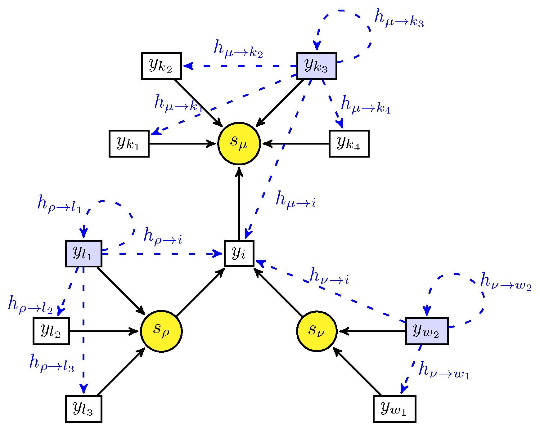
The detection problem that corresponds to (10) is shown in Figure 2. To this end, we proceed with the multi-source detection problem by setting it up as a problem in the context of a statistical mechanics system, where the system energy is E and the inverse temperature is β , serving as the “soft maximum” parameter. The total probability P ( y ) , which is the sum over all state vectors s , is called “partition function” Z , and it is expressed as
Z ( y ) = s μ exp β E
The corresponding Helmholtz free energy per spin is
F N = 1 N β ln Z N
Then, the above-mentioned optimization problem becomes equivalent to finding the state vector s that minimizes the above energy functional. This can be achieved directly by taking the limit β , i.e.,
s ^ = argmin s { 1 , + 1 } N E = lim β 1 N β ln Z
Similar arguments to the above can be also made if we generalize the domain of the state variables s i from binary to continuous.
The free energy is a random quantity depending on the realization of the network and the noise. However, it has been conjectured [50] (and proven in some cases) that it self-averages in the large system limit in the sense that
lim N F N = lim N E F N
If E depends on external “quenched” random variables, i.e., E ( s , G ) , then E min and F also depend on G . To evaluate the quantity E ln Z , where the expectation is taken with respect to G , y , T , R , we perform the replica trick, which can be expressed as
E ln Z = lim n 0 + 1 n ln E Z n
where it is assumed that the resulting expression holds when analytically continuing n 0 + . In summary, we can, therefore, make the following assumptions:
Assumption 1 
(Replica Assumption). E Z n evaluated for n N + can be analytically continued in the vicinity of n 0 + .
This assumption has seen widespread use in the field of statistical mechanics for alleviating the problem of dealing with averages of logarithms of random quantities since the logarithm is obtained after calculating Z n , as demonstrated in Appendix B.
Assumption 2 
(Interchanging Limits). The limits N and n 0 + in evaluating Z n can be interchanged.
The above assumptions enable us to obtain an expression for E Z n , which we need to evaluate using the saddle-point approximation. Here, we need to guess the right symmetries for the correct saddle-point solution. To do this, we invoke an additional assumption.
Assumption 3 
(Replica Symmetry). The correct saddle-point solution is symmetric under the permutation of replica indices.
Although quite appealing, this assumption is often incorrect. In fact, in several instances, it has been shown that the saddle-point solutions break replica symmetry [40]. Nevertheless, given the difficulty of evaluating the replica-symmetry-broken solution, it is customary in similar applications to proceed with the replica-symmetric assumption, which has been shown to yield results very close to the correct ones.

5. Results Using the Replica Approach

In this section, we describe how to obtain the results below using the replica approach, which constitutes the main results of this paper. For reasons of completeness, we analyze the replica method for our problem in Appendix B. For more details concerning the replica method, the interested reader is referred to [51,52,53].
We first average over the replicated partition function, i.e., E [ Z n ] (see (34)), assuming a random graph with a Poisson-distributed source-connectivity probability and SU-connectivity probability P k , with Poisson parameters T and R, respectively (see (5)). We also assume that the source-activity probability is P α (which, in simulations, we set to P α = 0.5 ), which means that each source is on with probability P α . In addition, we assume a Gaussian noise of strength σ 2 . After taking the replica-symmetry approximation, the fixed-point equations take a form similar to (17) and (24).
However, since the H and h ^ fields appearing are random, the fixed-point equations amount to the determination of their distributions in a self-consistent manner.
Equations (17) and (24) provide the (stochastic) relationship between the effective fields H and H ^ . As a result, at a steady state on the random graph where these quantities reside, their probability densities need to be related. In particular, by taking the limit of β , we obtain the following two basic recursive relations for their probability density, following [54]
Q ^ H ^ = lim β E G , z , R i = 1 R d H i Q ( H i ) δ H ^ ϵ β ( H )
with the expectation being over the realizations of the channel instantiation G , the noise z , and the number of SUs per source R and
Q H = E T k = 1 T 1 d H ^ k Q ^ H ^ k δ H k = 1 T 1 H ^ k
with T being the (random) number of sources per SU. It has been shown that both T and R follow the Poisson distribution determined by the average density of the sources and SUs in the network.
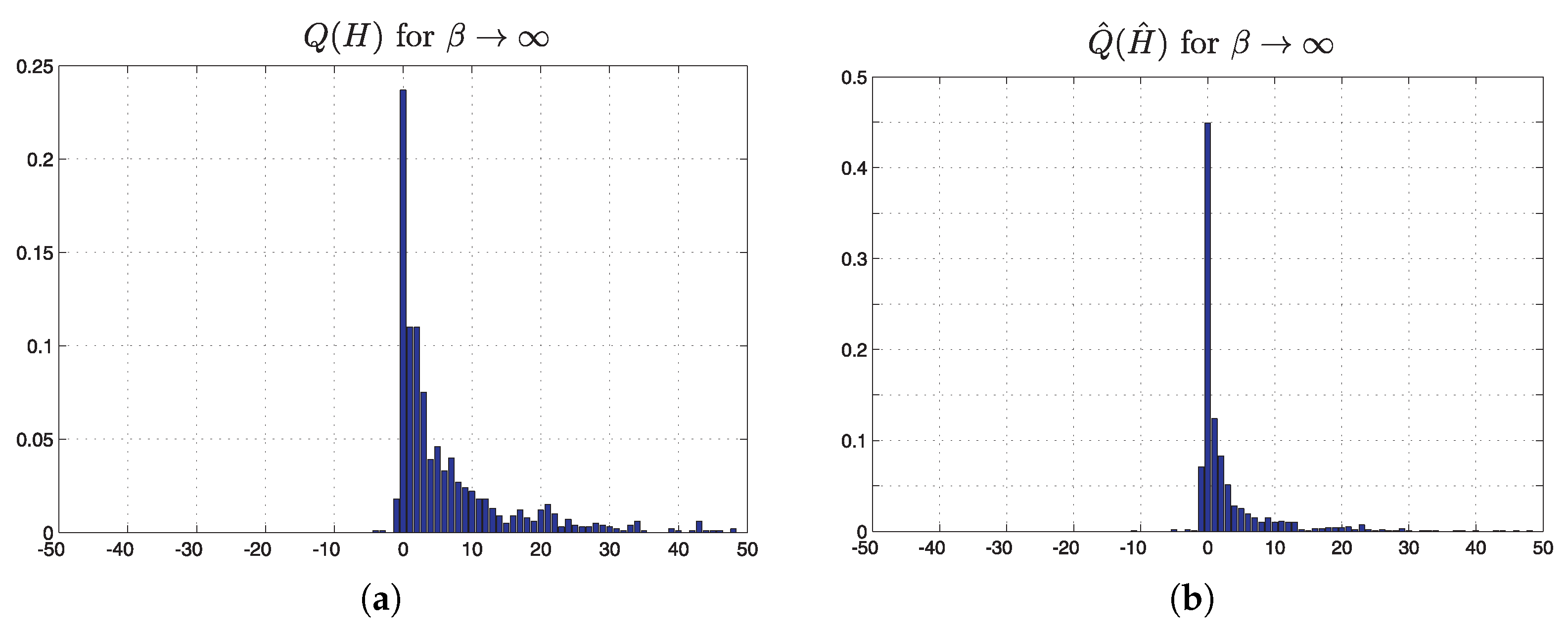
The probability of erroneous detection can be derived directly from the above distributions, (36) and (35), as depicted in Figure 3, and it can be written as
P err = 1 2 1 E H , H ^ sgn H + H ^
Equations (35)–(37) and the algorithm behind them, i.e., Algorithm 2, are the main results of this paper. The above error probability can be obtained by using population dynamics to calculate Q ( H ) and Q ^ ( H ^ ) , which solve the above distributional equations [22].
Algorithm 2 Population Dynamics (Graphical Model Ensemble, Resolution K, Number of Iterations I)
1:
Initialize { H i }
2:
for   i = 1 , , I   do
3:
      for  k = 1 , , K  do
4:
        Draw an integer t Poisson ( R ) .
5:
        Choose t 1 random samples from the H ^ bin and store their sum in the H bin.
6:
        Draw an integer r Poisson ( T ) .
7:
        Pull r random samples of the H bin.
8:
        Calculate the function tanh 1 [ ϵ β ] .
9:
        Pass the result to a randomly chosen element of the H ^ bin.
10:
     end for
11:
end for
Population dynamics can be analyzed by representing the effective field distributions by a large population of K copies (fields) randomly drawn from these two distributions. K is sufficiently large so as to provide good resolution in the desired performance measures [51]. As inputs, it requires the resolution K, the maximum number of iterations I, and a specification of the ensemble of the graphical model. The latter is needed for the description of the degree distributions between the sources and SUs and vice versa. The algorithmic procedure is described below.
First, we create K random values for H and K random samples for H ^ . Using these samples, we take at random t 1 random samples from the H ^ bin and store their sum at a random location in the H bin, where t is a random number obtained from the Poisson distribution, with the parameter R corresponding to the Erdős–Rényi random graph. We then generate a random T-Poisson-distributed number r and pull r random samples from the H bin, which are then used to evaluate the function tanh 1 [ ϵ β ( H ) ] , and we associate this number with a randomly chosen element in the H ^ bin. This procedure is iterated until the distributions of H ^ and H cease to vary over time.
As we can see, Equations (17) and (24) are at the heart of the above algorithm. When this message-passing approach converges to a steady state, the population and resulting empirical distributions, Q ( H ) and Q ^ ( H ^ ) , no longer vary. The distributions of fields H and H ^ for β = are depicted in Figure 3.
It should be noted that the probability of error (37) includes only cases where there is connectivity of each source with at least one SU. Thus, to normalize the source-outage probability by taking this observation into account, we must consider the probability of a primary source being completely unconnected to the secondary network, which is simply P unc = exp R . Taking this into account, the resulting total error detection rate can be written as
P total = P unc + 1 P unc P err
In concluding this section, it is worth summarizing the results [23]. First, we applied the message-passing algorithm to reliably detect the operational state of primary sources in a large random wireless network. At the same time, we developed an analytic methodology based on statistical physics, which obtains the probability of error of such an algorithm subject only to the statistical characteristics of the network. This analytic framework inputs the densities of primary users and secondary users, as well as the statistics of the propagation environment. From these inputs, it calculates the (Poisson) distribution of the connectivity of the bipartite network of primary users and SUs. Including the thermal noises in the detection process results in Equations (36) and (35), which then determine the densities Q ( H ) and Q ^ ( H ^ ) of the effective message fields for such a resulting bipartite random graph. From the above densities, we finally derive the probability of error detection in (37) and then (38).

6. Simulation Results

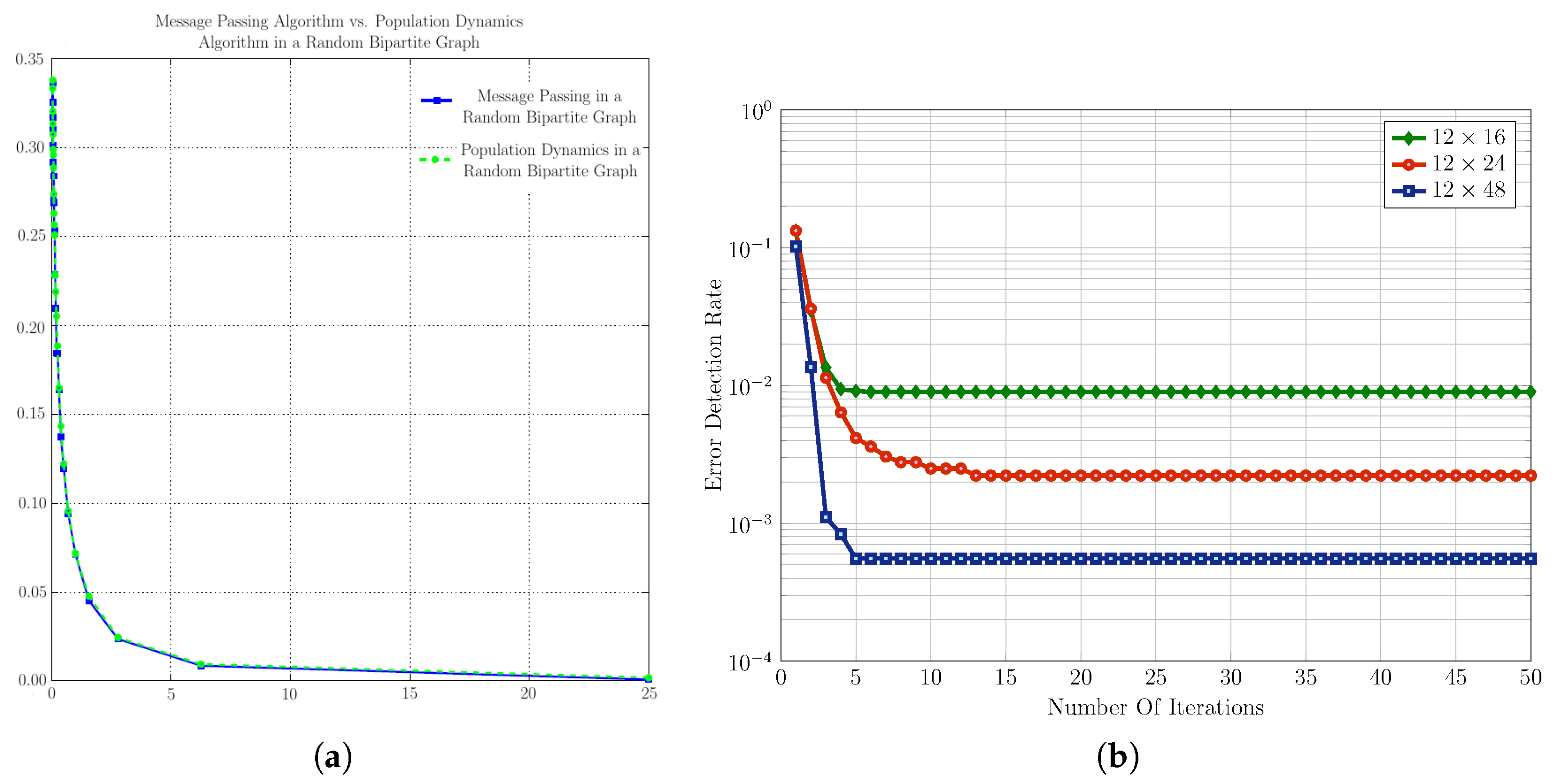
In this section, we numerically generate instances of two-dimensional primary-secondary networks with the aim of validating the above-discussed algorithm. The parameters and their values used in all the simulation scenarios can be seen in Table 4, where only the path-loss coefficient and the probability of a source being active have fixed values γ = 4 and P α = 0.5 , respectively, without loss of generality. The communication range, along with the average densities of the primary sources and SUs in a certain area, varies in each case to capture the fluctuations of the error detection rate. We start by showing that the proposed message-passing algorithm converges rapidly. Indeed, Figure 4b depicts the results from the simulation process regarding the convergence rate of the message-passing algorithm for various neighboring matrices, which differ not only in size, revealing the number of SUs and sources, but also in the connectivity between SUs and sources. As can be seen, the proposed algorithm converges very fast to the optimal solution. The SNR has been kept fixed, equal to SNR = 0 dB without loss of generality. The appealing aspect of our belief propagation algorithm is its linear complexity, which constitutes a competitive advantage compared to other algorithms.
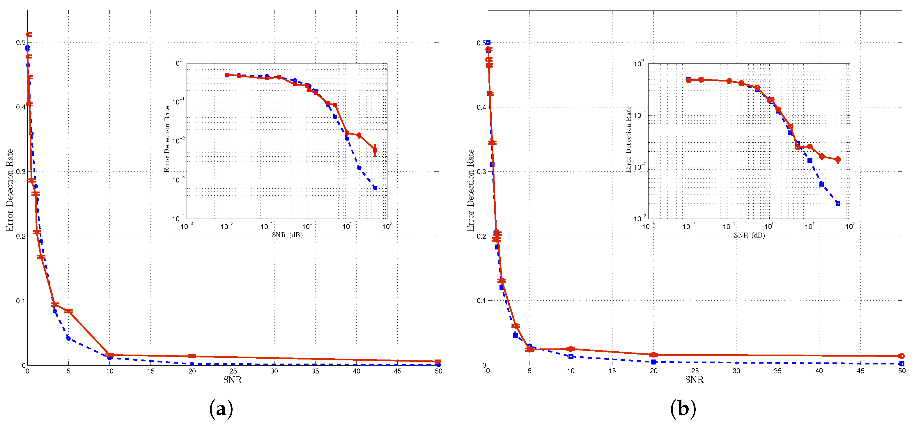
Next, we analyze the level of accuracy of the analytic approach from Equations (35) and (36), which are solved using population dynamics, and compare the results with an Erdős–Rényi random graph with the same parameters. Figure 4a depicts the error detection rate for the two algorithms we used, i.e., the message-passing and population dynamics algorithms. As can be seen, both algorithms demonstrate extremely good performance agreement.
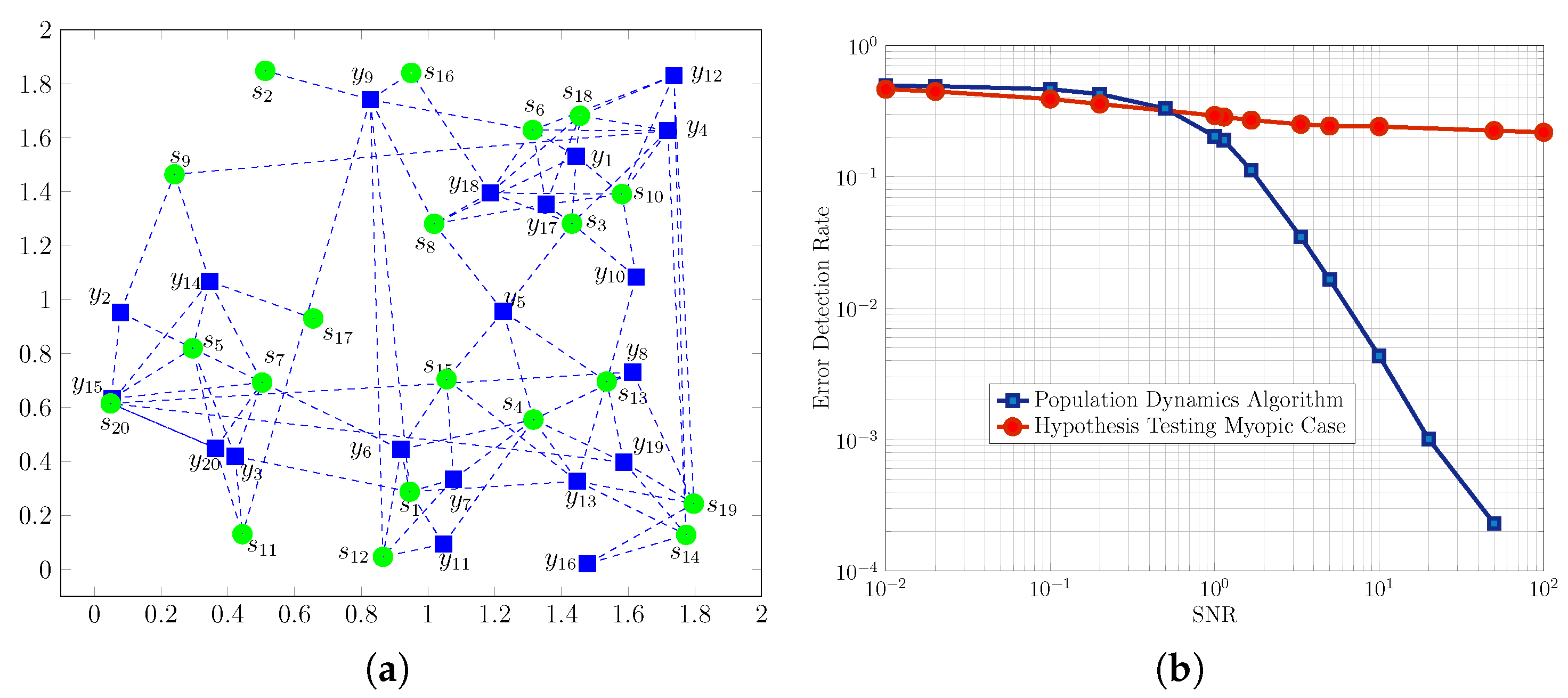
Further, it is important to compare the behavior of realistic two-dimensional networks. To this end, we generated 100 random instantiations of a network formed by 5 × 5 and 10 × 10 SUs and primary sources, respectively, with one such instantiation depicted in Figure 5a. The average error detection probability was evaluated for various values of the SNR using the population dynamics algorithm. Figure 6 shows a comparison of the two results with good agreement.
Interestingly, there is no phase transition, i.e., an error-free area, for the problem of multi-source detection. This can be easily demonstrated if one implements the message-passing algorithm with a strongly positive initial field (ferromagnetic) and compares it to the one with a random initial field (paramagnetic) [55]. In our case, there was no substantial difference in the value of the error detection rate, either for the dense case—where many sources were connected to a few SUs—or for the sparse case.
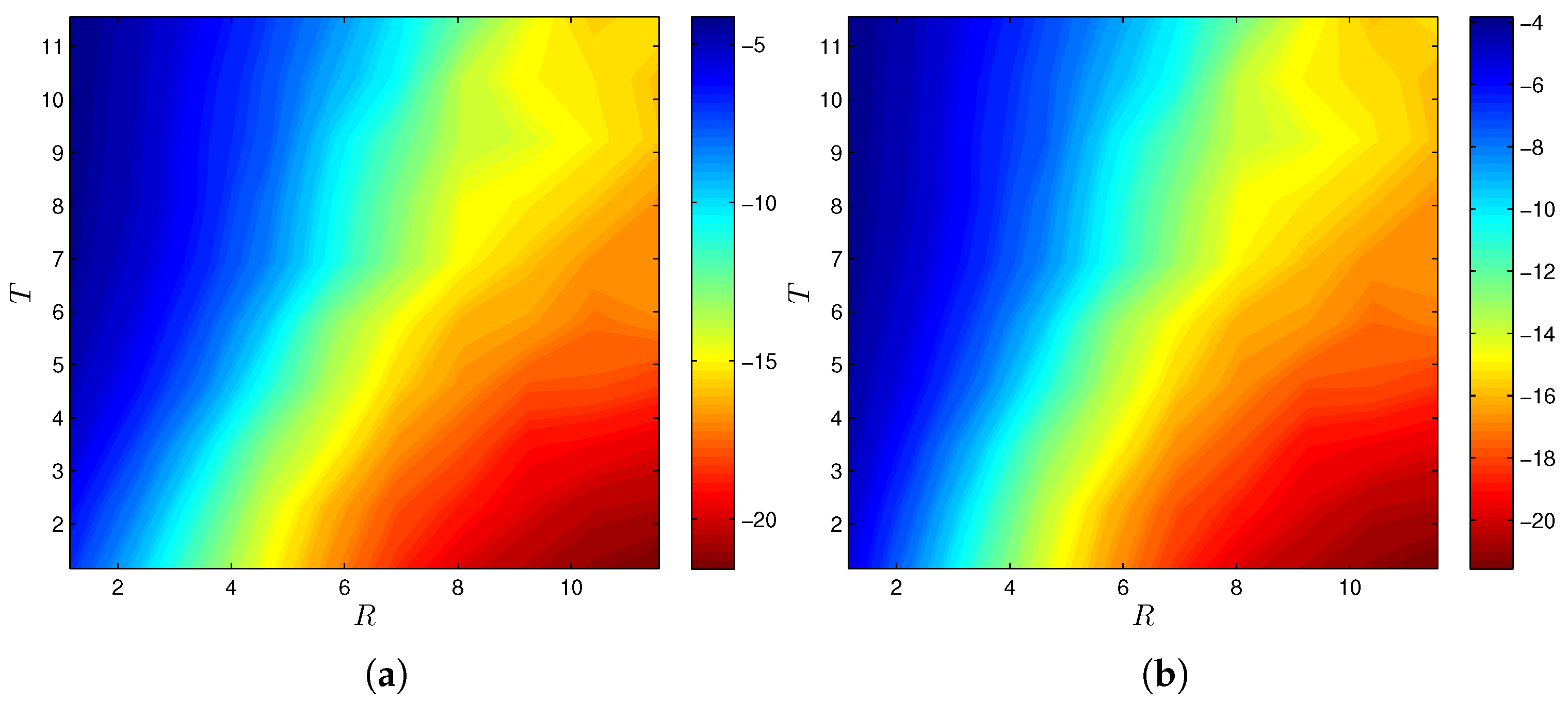
Finally, having justified the accuracy of the replica-symmetric approximation, we obtained the values of the error detection rate using the population dynamics algorithm for various values of T and R, as shown in Figure 7. On the left-hand side, we plot the probability of error, given that the source is connected to some SU, i.e., P err . Here, we find the approximate symmetry around the line T = R ; above that, the error is higher, whereas below that, the error is much lower. The figure on the right-hand side shows the total value of error P tot . We can see that for this set of parameter values, the detection rate is dominated by the probability of non-connection. As an SU’s density n s increases, the probability of non-connectivity is expected to decrease since more SUs in the same area yield better connectivity conditions between SUs and sources. Thus, both of the diagrams will have similar behavior, and we can constrain the error detection rate analysis to the case of P err .
The below Figure 7 depicts the results of our work, as it provides insights into how dense a wireless network should be for adequate source detection. Given some parameters such as the SU and source density, the communication range of the SUs, and the desired SNR , one can simply estimate the error detection probability. For example, if we have a density of R = 6 SUs/area and a fixed SNR = 0 dB, we can increase the detection reliability by almost 2 dB by taking R to be 7 instead of 6. Additionally, from a different perspective, if we have a density of T = 5 sources/area, increasing R by a factor of 1 will result in a substantial decrease in the error detection rate.
Concluding our discussion of the simulation results, we point out the use of diagrams or error detection maps, such as the one in Figure 7, to determine how dense the connections between SUs and sources should be for a given SNR . In practice, they can be used to determine how many SUs should be scattered in a field of interest so that all emitting sources in the field can be adequately detected.
Surprisingly, the fact that we modeled our system to behave well when the network forms a loop-less Cayley tree seemed not to be exceedingly important. Despite the fact that in our randomly instantiated two-dimensional networks, the neighborhood matrices contained many short loops, this did not substantially degrade the overall network performance. Additionally, we did not notice any phase transitions that could pose algorithmic barriers to the multi-source detection problem.

7. Comparison with the Case of Myopic SUs

In this section, we consider the detection problem in a network of myopic SUs, which are users that are capable of covering only one source at a time. As a consequence, the complexity is reduced; however, at the price of a considerable performance loss, as we will demonstrate. For this case, we formulate the problem and show through simulation results that it performs poorly in the case of intensive connectivity.
In a relatively dense environment, each SU receives a signal from several sources. A naive approach to detecting whether one source emits is to find the nearest SU to the specific source and rely only on this user for the detection process.
The SU uses a simple binary Neyman–Pearson hypothesis testing based on its (aggregated) received signal strength. If we denote SU y i to be the nearest user to source s μ , then the observations under the two different hypotheses are given by
y i = G i μ + ν N ( i ) μ G i ν s ν + η i , H 1 G i μ + ν N ( i ) μ G i ν s ν + η i , H 0
where H 1 denotes the emitting hypothesis ( s μ = + 1 ) and H 0 is the null hypothesis ( s μ = 1 ). Therefore, the likelihood under hypothesis H 1 is
P ( y i | H 1 ) = 1 2 π σ i 2 exp 1 2 σ i 2 y i G i μ 2
and, respectively, under hypothesis H 0 is
P ( y i | H 0 ) = 1 2 π σ i 2 exp 1 2 σ i 2 y i + G i μ 2
The logarithmic likelihood ratio test is then given by
L ( y i ) = log P ( y i | H 1 ) P ( y i | H 0 ) H 0 H 1 τ
where the SU decides, according to a threshold τ . Different criteria can be used to find the optimal threshold, but we do not deal with this topic in this paper.
The above-mentioned analysis shows that the multi-source detection task based on the measurements of the energy intensity field is a very hard problem since each measurement is composed of information from all individual sources.
Due to the nonlinearity of the energy intensity with respect to the distance, it is very difficult to decode each individual component [56]. In Figure 5b, a comparison of the aforementioned analysis for the myopic case detection and the population dynamics algorithm is depicted. It can be seen that the population dynamics algorithm and the message-passing algorithm (since their behavior is very similar) are superior to the simple scenario of the myopic SU detection of a single source.

8. Discussion and Conclusions

This paper presented an analytical study of detecting the transmitting state of multiple sources using a secondary user network in the presence of noise. We employed tools from statistical mechanics, namely the replica approach, to calculate the error detection rate for the network and showed that its results were in numerical agreement with those of the message-passing approach. Based on these results, we were able to analyze and quantitatively predict the error detection behavior in large-scale networks using only a few parameters related to the statistical characteristics of the connections, such as SUs’ and primary sources’ density, path loss exponent, and fading, which was the main novelty of this paper. Furthermore, driven by the need for a practical network implementation, we introduced a general framework for mapping our bipartite graph to a network structure. The entire framework we developed is fully distributed and presents an excellent approximation to the inference solution.
In the future, we intend to expand this approach to fault detection and diagnosis in sensor networks, i.e., the identification of faulty sensors or sensors with abnormal behavior, incorporating the dependencies between sensor signals. In parallel, we expect to modify the proposed framework by targeting the prediction of the powers of the primary sources. In this case, the exchanged messages are real-valued variables and thus differentiate most of the aspects of our analysis.
Additionally, we could extend our results to wireless networks where the sources emit dynamically, i.e., in several time frames. This scenario introduces the time variable into our problem of multi-source detection, creating a structured graph with many short loops, Therefore, it requires a new methodology. Interesting applications of the proposed framework include sensor localization, where neighboring sensor nodes exchange information based on the received signal strength; time of arrival; or other localization-related measurements. Apart from the sensor-localization application, which constitutes a direct continuation of our work, we plan to introduce the statistical mechanics-inspired solution to the target-localization problem, where belief propagation can be deployed to estimate the trajectory or current location of a moving target in a wireless sensor network.
Finally, as an interesting approach to detecting the emitting state of sources in a sensor network, we plan to combine the belief propagation algorithm with hidden Markov models to target improved inference in more complex graphical structures. Belief propagation can propagate beliefs through the HMM’s graphical structure, allowing for a more accurate estimation of the hidden states and model parameters. Moreover, the belief propagation algorithm can effectively deal with noisy or missing data in the observation sequence and thus compensate for the uncertainties in the observed data.

Author Contributions

Conceptualization, S.E. and A.L.M.; methodology, A.L.M. and S.E.; validation, S.E. and A.L.M.; formal analysis, S.E. and A.L.M.; resources, S.E. and A.L.M.; data curation, S.E.; writing—original draft preparation, S.E. and A.L.M.; writing—review and editing, A.L.M.; visualization, S.E.; supervision, A.L.M.; project administration, S.E.; funding acquisition, S.E. All authors have read and agreed to the published version of the manuscript.

Funding

This research was funded by the European Union’s Horizon 2020 research and innovation program under grant agreement number 957406 (TERMINET).

Conflicts of Interest

The authors declare no conflict of interest. The funders had no role in the design of the study; in the collection, analyses or interpretation of data; in the writing of the manuscript; or in the decision to publish the results.

Appendix A. Network Implementation of the MP Algorithm
Along with the performance of the message-passing detection algorithm, it is important to describe how this algorithm can be implemented in an SU network. Despite the distributed nature of belief propagation methods, their implementation in a particular network structure is not necessarily obvious [57]. In this section, we provide a simple protocol for distributing information in SU networks in the context of the message-passing algorithm.
We assume that at any given step of the iteration, the ith SU has local measurement and channel information y i , G i ν , as well as the messages h ν i , for all neighboring sources ν available. From this, it can calculate the messages h ^ i ν using (24). It can then transmit each of the h ^ i ν to a designated SU connected with source ν . This designated SU can then sum over all received h ^ j ν for j N ( ν ) and then broadcast the resulting sum j h ^ j ν to all SUs connected to ν . In the next step, each SU i can obtain the revised value of h ν i by subtracting its own h ^ i ν , as seen in (17).
The choice of the above designated SU for each source should be made to minimize the total network communication energy consumption. In general, this is not trivial to determine, so we propose a suboptimal criterion, namely the nearest SU neighboring each source. This choice makes sense because this SU has the larger probability of including in its communication range all the other SUs the source is connected to. Additionally, assuming a semi-static topology, these two nodes of the bipartite graph will probably have a high-quality communication link between them (see Figure 2).
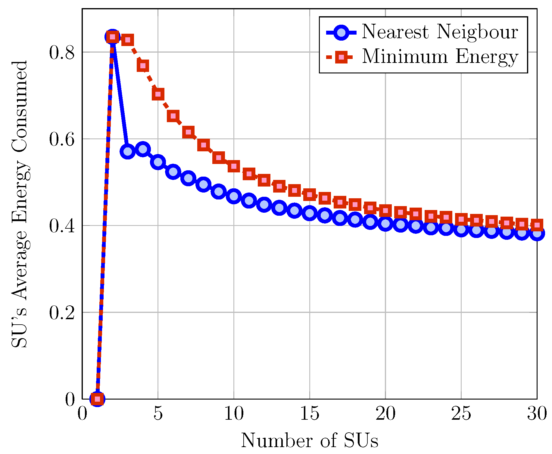
In Figure A1, we compared the average SU energy consumed for the case where the chosen SU is the nearest neighbor of the source, i.e., the SU that has the minimum Euclidean distance from the source, with the case where the SU is the true SU, which minimizes the total energy consumed in the network, which is expressed for simplicity as
E 0 = min j E j = min j i = 1 k d i j γ
where E j is the energy for every SU j for the case where the signal is degraded due to path loss. It can be readily seen that these two different schemes behave very similarly and, especially for a large number of nodes, they tend to consume the same amount of power.
Figure A1. Average energy of an SU consumed as a function of the number of SUs participating in the network formation. We generated 10,000 instantiations of different networks formed by k SUs, with k = 1 , , 30 , randomly dropped inside a circular area with a radius equal to the SU’s communication range ( r c = 0.5 ). It can be observed that for highly dense environments, where the connectivity between SUs is large, these two schemes yield similar results, considering signal power degradation due to path loss.
Telecom 04 00029 g0a1

Appendix B. The Replica Method

In this section, we provide the detailed replica calculation. We start with (30), which can be re-written as
Z ( y | T μ , R i ) = s ( a ) exp β 2 i ε i s ν N ( i )
where
ε i s ν N ( i ) = y i ν N ( i ) G i ν A i ν s ν 2
    y i = ν N ( i ) G i ν A i ν s ν 0 + η i
and T μ and R i are the source and SU connectivities, respectively, and A is the adjacency matrix, with the elements A i ν = 1 if a link between source ν and SU i exists and 0 otherwise.
The graphs considered in this paper are described by a fixed ratio of the number of sources to the number of SUs, or equivalently, the ratio of the mean SU node connectivity to the mean source node connectivity
ϱ = K M = T R .
A prior distribution on the edges for the Erdős–Rényi (sparse) graph model is given by
P A i ν | T , R = 1 T K δ A i ν , 0 + T K δ A i ν , 1
where δ is the Kronecker delta function.
To proceed with the replica method, we introduce the replica index a for the total n replicas of the partition function. This way, we can express the exponential term of (A2) as
Z n = s ( a ) exp β 2 i , a ε i s ν N ( i ) ( a ) = s ( a ) i = 1 K a = 1 n d ϵ a i 2 π exp ϵ a i 2 2 exp i β a = 1 n ϵ a i η i + ν N ( i ) G i ν A i ν s ν 0 s ν ( a )
or equivalently,
Z n = s ( a ) i = 1 K a = 1 n D ϵ a i exp i β ϵ a i η i ν , i exp i β G i ν A i ν a ϵ a i s ν 0 s ν ( a ) .
In the expression above, we have performed the Hubbard–Stratonovich transformation [58] to express the square term in the exponent as a linear term at the expense of introducing the additional variable ϵ ( a )
exp χ 2 2 = + d ϵ 2 π exp ϵ 2 2 + i ϵ χ .
For reasons of notational simplicity, we have also introduced D ϵ ( a ) , which is connected to the ϵ ( a ) variable in the following way
D ϵ ( a ) = d ϵ ( a ) 2 π exp ϵ ( a ) 2 2 .
The average replicated partition function can now be evaluated as
E Z n = { s ν } P s ν 0 i = 1 K a D ϵ a i exp i β ϵ a i η i × i , ν E A i ν E G i ν exp i β A i ν G i ν a = 1 n ϵ a i s ν 0 s ν ( a )
At this point, we denote
g i ν = g i ( s ν ) = E G exp i β G a = 1 n ϵ a , i s ν 0 s ν ( a )
and impose the source and SU connectivity constraints using the Cauchy integral formula
T ν δ i = 1 K A i ν T ν = T ν 1 2 π i d τ ν τ ν T ν + 1 i = 1 K τ ν A i ν
R i δ ν = 1 M A i ν R i = R i 1 2 π i d ω i ω i R i + 1 ν = 1 M ω i A i ν
where the integrals are around unit circles in the complex plane, centered at zero. In (A11), we average over A i ν and obtain
i , ν E A i ν g i A i ν = i = 1 K R i = 0 M d ω i 2 π i ω i R i + 1 ν = 1 M T ν = 0 K d τ ν 2 π i τ ν T ν + 1 i , ν E A i ν g i ν ω i τ ν A i ν = i = 1 K R i = 0 M d ω i 2 π i ω i R i + 1 ν = 1 M T ν = 0 K d τ ν 2 π i τ ν T ν + 1 i , ν 1 R M + R M g i ν ω i τ ν
Approximating to leading order the last parenthesis as exp T K g i ν ω i τ ν 1 and performing the Cauchy integral, results in the selection of the T ν -th term in the expansion of the i-product, so
i , ν E A i ν g i A i ν = ν = 1 M T ν d τ ν 2 π i τ ν T ν + 1 × i = 1 K R i exp R R R i R i ! 1 M ν g i ν τ ν R i .
To extract the ν -th dependence of the above expression, we introduce the auxiliary functionals Φ σ and Φ ^ ( σ ) of σ ( a ) at each site a = 1 , , n and then define δ σ , s ν as
δ σ , s ν = a = 0 n δ σ ( a ) , s ν ( a ) .
In this way, the dynamical variable dependence is expressed as
d Φ ( σ ) δ Φ ( σ ) 1 M ν = 1 M τ ν δ σ , s = 1 ,
and (A16) becomes
i , ν E A i ν g i ν A i ν = d Φ ( σ ) d Φ ^ ( σ ) exp T M σ Φ ( σ ) Φ ^ ( σ ) × ν = 1 M d τ ν 2 π i τ ν T ν + 1 exp T τ ν Φ ^ ( s ν ) i = 1 K exp [ R ] R R i R i ! l = 1 R i σ l Φ ( σ l ) g i σ l .
The next step is to integrate over τ ν and obtain
ν = 1 M d τ ν τ ν T ν + 1 exp T τ ν Φ ^ ( s ν ) = ν = 1 M T T ν T ν ! Φ ^ ( s ν ) T ν
Note that the last term in (A19) has an ϵ a ν -dependence and it can be integrated out, so
i = 1 K R i exp [ R ] R R i R i ! l = 1 R i σ l Φ ( σ l ) g i ν = l = 1 R i σ l Φ σ l exp β 2 a = 1 n η + l = 1 R i G l σ l 0 σ l ( a ) 2 = i , a D ϵ a i exp i β ϵ a i η i i exp R R R i R i ! { σ l } l = 1 R i Φ σ l g i σ l i exp R R R i R i ! { σ l } l = 1 R i Φ σ l E η , g exp β 2 a = 1 n η l = 1 R i g l σ l 0 σ l ( a ) 2
The replicated partition function defined in (A11) after integrating over ϵ a i , can then be decomposed into three terms as
E Z n σ d Φ ( σ ) d Φ ^ ( σ ) exp G 1 G 2 G 3
where
G 1 = T M σ Φ ( σ ) Φ ^ ( σ )
G 2 = K ln E R i , G , η l = 1 R i σ l Φ σ l exp β 2 a = 1 n η + l = 1 R i G l σ l 0 σ l ( a ) 2
G 3 = T M M ln s ν P s ν 0 E T ν Φ ^ ( s ν ) T ν
In (A24), the average over R i is taken using the Poisson distribution
P R R i = R R i R i ! exp R
Similarly, for the average over T ν in (A25),
P T T ν = T T ν T ν ! exp T .
Since G 1 , G 2 , and G 3 are all O ( N ) , (A22) can be evaluated using the saddle-point analysis [59]. At the saddle point, the self-averaged free energy can be written as
β F = lim n 0 n extr Φ , Φ ^ G 1 Φ , Φ ^ G 2 Φ G 3 Φ ^
A tractable form for the saddle-point equations is attained using the RS assumption, which is
Φ ( σ ) = d h Q ( h ) exp σ 0 β h a = 1 n σ ( a ) 2 n cosh n ( β h )
In this way, by plugging (A29) into (A22), for each separate term, we obtain
G 1 ( n ) = T M σ d h d h ^ Q ^ ( h ^ ) Q ( h ) exp β h σ 0 a σ a exp β h ^ σ 0 a σ a 2 cosh ( β h ) n 2 cosh ( β h ^ ) n = T M σ d h Q ( h ) d h ^ Q ^ ( h ^ ) 2 cosh ( β h + h ^ n 2 cosh ( β h ) n 2 cosh ( β h ^ ) n = T M σ d h Q ( h ) d h ^ Q ^ ( h ^ ) 1 + n ln 2 cosh ( β h + h ^ 2 cosh ( β h ) 2 cosh ( β h ^ )
G 2 ( n ) = K ln E R i , G , η l = 1 R i σ l 0 d h l Q ( h l ) X n
where
X = σ 1 , , σ R i l = 1 R i exp β σ l 0 h l σ l 2 cosh β h l exp β 2 η + l = 1 R i G l σ l 0 σ l 2
Finally, by following the same procedure as before, we express G 3 ( n ) as
G 3 ( n ) = T M M ln [ W ]
where
W = E T ν k = 1 T ν d h ^ k Q ^ ( h ^ k ) 2 cosh β k = 1 T ν h ^ k k 2 cosh β h ^ k n = E T ν 2 T ν exp T 2 + E T ν k = 1 T ν d h ^ k 2 Q ^ ( h ^ k ) n ln 2 cosh β k = 1 T ν h ^ k k 2 cosh β h ^ k
so,
G 3 ( n ) = M T 2 n M E T ν k = 1 T ν d h ^ k 2 Q ^ ( h ^ k ln 2 cosh β k = 1 T ν h ^ k k 2 cosh β h ^ k
By taking the functional derivative with respect to Q ^ h ^ at n = 0 , we obtain
n δ G 1 ( n ) δ Q ^ h ^ | n = 0 = T M d h Q ( h ) ln 2 cosh β h + h ^ 2 cosh β h 2 cosh β h ^ = T M 2 d h Q ( h ) ln 1 + tanh ( β h ) tanh β h ^ 2
and
n δ G 3 ( n ) δ Q ^ h ^ | n = 0 = M k = 1 T ν 1 d h ^ k Q ^ ( h ^ k ) s ln 2 cosh β l = 1 T ν 1 h ^ l + h l = 1 T ν 2 cosh β h ^ l
Similarly, the functional derivative with respect to Q ( h ) is
n δ G 1 ( n ) δ Q h | n = 0 = T M d h ^ Q ^ h ^ ln 2 cosh β h ^ + h 2 cosh β h 2 cosh β h ^
and
n δ G 2 ( n ) δ Q h | n = 0 = K R l = 1 R i d h l Q ( h l ) σ l 0 P σ l 0 ln X
where we have used the following approximation
X n 1 + n ln X
The sum inside the exponential term of (A32) can be further analyzed as
l = 1 R i G l 1 σ l ( a ) 2 = G R i 1 σ R i + l = 1 R i 1 G l 1 σ l ( a ) 2
From (A36) and (A37), we obtain
d h ^ Q ( h ^ ) ln 2 cosh β h + h ^ = k = 1 T ν 1 d h ^ k Q ( h ^ k ) ln 2 cosh β h + j = 1 T ν 1 h ^ j
and if we set y = j = 1 T ν 1 h ^ j , the above expression results in
Q h = E T ν k = 1 T ν 1 d h ^ k Q ^ h ^ k δ h k = 1 T ν 1 h ^ k
Similarly, from (A38) and (A39), we obtain
d h ^ Q ^ h ^ ln cosh β h ^ + h = l = 1 R i d h l Q ( h l ) σ l 0 P σ l 0 ln X
To have a more compact form, we define
U + = σ l exp h l exp β η + l = 1 l R i R i G l 1 σ l 2
U = σ l exp h l exp β η + G R i 1 σ R i 2 + l = 1 R i 1 G l 1 σ l ( a ) 2
In this way, we can express h ^ as
h ^ = ln U + U
and obtain the Q ^ ( h ^ ) distribution
Q ^ h ^ = E R i j = 1 R i d h j Q ( h j ) δ h ^ ϵ β ( h )
which is (35) in Section 5.
The total error detection probability can be calculated by adding an effective magnetic field term in the cost function, E , of (29), so,
E E + δ μ = 1 M s μ s ^ μ
which modifies the G 3 term of the replicated partition function in (A8), resulting in
G 3 = k = 1 T ν d h ^ k Q ^ ( h ^ k ) × 2 cosh k h ^ k β δ k 2 cosh h ^ k n = T M M ln E T ν E h ^ 2 cosh k h ^ k β δ k 2 cosh h ^ k n
After taking the partial derivative of G 3 with respect to the distribution Q ^ h ^ , we obtain
δ G 3 δ Q ^ h ^ = M E T ν k = 1 T ν 1 Q ^ h ^ k ln 2 cosh k T ν 1 h ^ k + h ^
As a final step, we take the partial derivative of F with respect to δ for δ 0 ,
F δ = 1 β δ G 3 ( δ ) | δ = 0 = M E T ν E h ^ sign k = 1 T ν h ^ k = M d h d h ^ Q ( h ) Q ^ h ^ sign h + h ^
which validates the results in [23] obtained using the Bethe approximation.

References

  1. Gharib, A.; Ejaz, W.; Ibnkahla, M. Distributed Spectrum Sensing for IoT Networks: Architecture, Challenges, and Learning. IEEE Internet Things Mag. 2021, 4, 66–73. [Google Scholar]
  2. Idrees, Z.; Usman, M.; Gelani, H.E.; Zheng, L. Fast and Robust Spectrum Sensing for Cognitive Radio Enabled IoT. IEEE Access 2021, 9, 165996–166007. [Google Scholar]
  3. Xu, Y.; Gui, G.; Gacanin, H.; Adachi, F. A Survey on Resource Allocation for 5G Heterogeneous Networks: Current Research, Future Trends, and Challenges. IEEE Commun. Surv. Tutor. 2021, 23, 1668–1695. [Google Scholar]
  4. Li, F.; Lam, K.-Y.; Li, X.; Sheng, Z.; Hua, J.; Wang, L. Advances and Emerging Challenges in Cognitive Internet-of-Things. IEEE Trans. Ind. Inform. 2020, 16, 5489–5496. [Google Scholar]
  5. Awin, F.A.; Alginahi, Y.M.; Abdel-Raheem, E.; Tepe, K. Technical Issues on Cognitive Radio-Based Internet of Things Systems: A Survey. IEEE Access 2019, 7, 97887–97908. [Google Scholar]
  6. Rodriguez, A.C.S.; Haider, N.; He, Y.; Dutkiewicz, E. Network Optimisation in 5G Networks: A Radio Environment Map Approach. IEEE Trans. Veh. Technol. 2020, 69, 12043–12057. [Google Scholar]
  7. Adams, D.C.A.L.; Uher, J. Secondary Spectrum Usage and Signal Detection. In Wireless Coexistence: Standards, Challenges, and Intelligent Solutions; IEEE: Piscataway, NJ, USA, 2021; pp. 115–154. [Google Scholar]
  8. Maleki, N.; Vosoughi, A.; Rahnavard, N. Distributed Binary Detection Over Fading Channels: Cooperative and Parallel Architectures. IEEE Trans. Veh. Technol. 2016, 65, 1759–1765. [Google Scholar] [CrossRef]
  9. Huang, Q.; Chung, P.J.; Thompson, J. A nonparametric approach for spectrum sensing using bootstrap techniques. In Proceedings of the IEEE Global Communications Conference, Austin, TX, USA, 8–12 December 2014; pp. 851–856. [Google Scholar]
  10. Pearl, J. Probabilistic Reasoning in Intelligent Systems: Networks of Plausible Inference; Morgan Kaufmann Publishers Inc.: San Francisco, CA, USA, 1988. [Google Scholar]
  11. Zekavat, R.; Buehrer, R.M. Belief Propagation Techniques for Cooperative Localization in Wireless Sensor Networks. In Handbook of Position Location: Theory, Practice, and Advances; IEEE: Piscataway, NJ, USA, 2019; pp. 967–998. [Google Scholar]
  12. Murphy, K.P.; Weiss, Y.; Jordan, M.I. Loopy belief propagation for approximate inference: An empirical study. In Proceedings of the Fifteenth Conference on Uncertainty in Artificial Intelligence (UAI’99); Morgan Kaufmann Publishers Inc.: San Francisco, CA, USA, 1999; pp. 467–475. [Google Scholar]
  13. Sudderth, E.B.; Ihler, A.T.; Isard, M.; Freeman, W.T.; Willsky, A.S. Nonparametric belief propagation. In Commun. ACM 53, 10; Association for Computing Machinery: New York, NY, USA, 2010; pp. 95–103. [Google Scholar]
  14. Riegler, E.; Kirkelund, G.; Manchon, C.; Badiu, M.; Fleury, B. Merging Belief Propagation and the Mean Field Approximation: A Free Energy Approach. IEEE Trans. Inf. Theory 2013, 59, 588–602. [Google Scholar]
  15. Cakmak, B.; Winther, O.; Fleury, B. S-AMP: Ap2014 IEEE Information Theory Workshop (ITW 2014) proximate Message Passing for General Matrix Ensembles. In Proceedings of the 2014 IEEE Information Theory Workshop (ITW), Hobart, TAS, Australia, 2–5 November 2014; pp. 192–196. [Google Scholar]
  16. Rangan, S.; Fletcher, A.; Goyal, V. Asymptotic Analysis of MAP Estimation Via the Replica Method and Applications to Compressed Sensing. IEEE Trans. Inf. Theory 2012, 58, 1902–1923. [Google Scholar]
  17. Kabashima, Y. A CDMA Multiuser Detection Algorithm on the Basis of Belief Propagation. J. Phys. Math. Gen. 2003, 36, 11111. [Google Scholar] [CrossRef]
  18. Korada, S.; Montanari, A. Applications of the Lindeberg Principle in Communications and Statistical Learning. IEEE Trans. Inf. Theory 2011, 57, 2440–2450. [Google Scholar]
  19. Kabashima, Y.; Wadayama, T.; Tanaka, T. Statistical Mechanical Analysis of a Typical Reconstruction Limit of Compressed Sensing. In Proceedings of the 2010 IEEE International Symposium on Information Theory, Austin, TX, USA, 13–18 June 2010; pp. 1533–1537. [Google Scholar]
  20. Donoho, D.L.; Maleki, A.; Montanari, A. Message-passing Algorithms for Compressed Sensing. Proc. Natl. Acad. Sci. USA 2009, 106, 18914–18919. [Google Scholar] [CrossRef]
  21. Tesfamicael, S.A.; Godana, B.E. Compressed Sensing Performance Analysis via Replica Method Using Bayesian Framework. In Proceedings of the 17th UKSim-AMSS IEEE International Conference on Modelling and Simulation (UKSim), Cambridge, UK, 25–27 March 2015; pp. 281–289. [Google Scholar]
  22. Mézard, M.; Montanari, A. Information, Physics, and Computation; Oxford University Press: New York, NY, USA, 2009. [Google Scholar]
  23. Evangelatos, S.; Moustakas, A. Statistical Mechanics Approach for the Detection of Multiple Wireless Sources via a Sensor Network. In Proceedings of the IEEE 12th International Symposium on Modeling and Optimization in Mobile, Ad Hoc and Wireless Networks (WiOpt), Hammamet, Tunisia, 12–16 May 2014; pp. 591–598. [Google Scholar]
  24. Leon-Garcia, F.; Palomares, J.; Olivares, J. D2R-TED: Data—Domain Reduction Model for Threshold-Based Event Detection in Sensor Networks. Sensors 2018, 18, 3806. [Google Scholar] [CrossRef]
  25. Abdul-Salaam, G.; Abdullah, A.H.; Anisi, M.H. Energy-Efficient Data Reporting for Navigation in Position-Free Hybrid Wireless Sensor Networks. IEEE Sens. J. 2017, 17, 2289–2297. [Google Scholar] [CrossRef]
  26. Lewandowski, M.; Płaczek, B. Data Transmission Reduction in Wireless Sensor Network for Spatial Event Detection. Sensors 2021, 21, 7256. [Google Scholar] [CrossRef]
  27. Cobos, M.; Perez-Solano, J.J.; Felici-Castell, S.; Segura, J.; Navarro, J.M. Cumulative-Sum-Based Localization of Sound Events in Low-Cost Wireless Acoustic Sensor Networks. IEEE/Acm Trans. Audio Speech, Lang. Process. 2014, 22, 1792–1802. [Google Scholar] [CrossRef]
  28. Miao, J.; Song, X.O. An Enhanced Soft Combination Algorithm Based on CUSUM for Cooperative Spectrum Sensing. In Proceedings of the 2017 IEEE International Conference on Networking and Network Applications (NaNA), Kathmandu, Nepal, 16–19 October 2017; pp. 176–179. [Google Scholar]
  29. Jain, A.; Sarvepalli, P.; Bhashyam, S.; Kannu, A.P. Algorithms for Change Detection With Sparse Signals. IEEE Trans. Signal Process. 2020, 68, 1331–1345. [Google Scholar] [CrossRef]
  30. Bai, Y.; Wang, X.; Jin, X.; Zhao, Z.; Zhang, B. A Neuron-Based Kalman Filter with Nonlinear Autoregressive Model. Sensors 2020, 20, 299. [Google Scholar] [CrossRef]
  31. Zhang, M.; Li, X.; Wang, L. An Adaptive Outlier Detection and Processing Approach Towards Time Series Sensor Data. IEEE Access 2019, 7, 175192–175212. [Google Scholar] [CrossRef]
  32. Mor, B.; Garhwal, S.; Kumar, A. A Systematic Review of Hidden Markov Models and Their Applications. Arch. Comput. Methods Eng. 2021, 28, 1429–1448. [Google Scholar] [CrossRef]
  33. Joshi, S.S.; Phoha, V.V. Investigating hidden Markov models capabilities in anomaly detection. In Proceedings of the 43rd Annual Southeast Regional Conference—Volume 1 (ACM-SE 43), Association for Computing Machinery, New York, NY, USA, 18–20 March 2005; pp. 98–103. [Google Scholar]
  34. Tuğaç, S.; Efe, M. Hidden Markov Model based target detection. In Proceedings of the 13th IEEE International Conference on Information Fusion, Edinburgh, UK, 26–29 July 2010; pp. 1–7. [Google Scholar]
  35. Adhikary, A.; Nam, J.; Ahn, J.-Y.; Caire, G. Joint Spatial Division and Multiplexing—the Large-scale Array Regime. IEEE Trans. Inf. Theory 2013, 59, 6441–6463. [Google Scholar] [CrossRef]
  36. Hata, M. Empirical Formula for Propagation Loss in Land Mobile Radio Services. IEEE Trans. Veh. Technol. 1980, 29, 317–325. [Google Scholar] [CrossRef]
  37. Bickson, D.; Baron, D.; Ihler, A.; Avissar, H.; Dolev, D. Fault Identification Via Nonparametric Belief Propagation. IEEE Trans. Signal Process. 2011, 59, 2602–2613. [Google Scholar] [CrossRef]
  38. Franceschetti, M.; Meester, R. Random Networks for Communication; Cambridge University Press: Cambridge, UK, 2007. [Google Scholar]
  39. Kirkley, A.; Cantwell, G.T.; Newman, M.E.J. Belief propagation for networks with loops. Sci. Adv. 2021, 7, eabf1211. [Google Scholar] [CrossRef] [PubMed]
  40. Mézard, M.; Parisi, G.; Virasoro, M.A. Spin Glass Theory and Beyond; World Scientific Publishing Company: Singapore, 1987. [Google Scholar]
  41. Talagrand, M. Spin Glasses: A Challenge for Mathematicians: Cavity and Mean Field Models; Springer Science & Business Media: Berlin/Heidelberg, Germany, 2003. [Google Scholar]
  42. Saad, D.; Yeung, C.; Rodolakis, G.; Syrivelis, D.; Koutsopoulos, I.; Tassiulas, L.; Urbanke, R.; Giaccone, P.; Leonardi, E. Physics-inspired Methods for Networking and Communications. IEEE Commun. Mag. 2014, 52, 144–151. [Google Scholar] [CrossRef]
  43. Guo, D.; Verdu, S. Replica Analysis of Large-system CDMA. In Proceedings of the 2003 IEEE Information Theory Workshop, Paris, France, 31 March–4 April 2003; pp. 22–25. [Google Scholar]
  44. Sourlas, N. Spin-glass Models as Error-correcting Codes. Nature 1989, 339, 693–695. [Google Scholar] [CrossRef]
  45. Mukherjee, K.; Gupta, S.; Ray, A.; Wettergren, T.A. Statistical-Mechanics-Inspired Optimization of Sensor Field Configuration for Detection of Mobile Targets. IEEE Trans. Syst. Man Cybern. Part Cybern. 2011, 41, 783–791. [Google Scholar] [CrossRef]
  46. MacKay, D.J.C. Information Theory, Inference & Learning Algorithms; Cambridge University Press: New York, NY, USA, 2002. [Google Scholar]
  47. Reeves, G.; Pfister, H.D. The replica-symmetric prediction for compressed sensing with Gaussian matrices is exact. In Proceedings of the 2016 IEEE International Symposium on Information Theory (ISIT), Barcelona, Spain, 10–15 July 2016; pp. 665–669. [Google Scholar]
  48. Decelle, A. An Introduction to Machine Learning: A perspective from Statistical Physics. Phys. Stat. Mech. Its Appl. 2022, 128154. [Google Scholar] [CrossRef]
  49. Bethe, H.A. Statistical theory of superlattices. Proc. R. Soc. London. Ser. -Math. Phys. Sci. 1935, 150, 552–575. [Google Scholar]
  50. Guerra, F.; Toninelli, F.L. The Thermodynamic Limit in Mean Field Spin Glass Models. Commun. Math. Phys. 2002, 230, 71–79. [Google Scholar] [CrossRef]
  51. Raymond, J.; Saad, D. Sparsely Spread CDMA—A Statistical Mechanics-based Analysis. J. Phys. Math. Theor. 2007, 40, 12315. [Google Scholar] [CrossRef]
  52. Monasson, R. Optimization Problems and Replica Symmetry Breaking in Finite Connectivity Spin Glasses. J. Phys. Math. Gen. 1998, 31, 513. [Google Scholar] [CrossRef]
  53. Vicente, R.; Saad, D.; Kabashima, Y. Low-density Parity-check Codes—A Statistical Physics Perspective. In ser. Advances in Imaging and Electron Physics; Peter, B.K., Hawkes, W., Mulvey, T., Eds.; Elsevier: Amsterdam, The Netherlands, 2003; Volume 125, pp. 231–353. [Google Scholar]
  54. Wong, K.Y.M.; Saad, D. Inference and Optimization of Real Edges on Sparse Graphs: A statistical Physics Perspective. Phys. Rev. E 2007, 76, 011115. [Google Scholar] [CrossRef] [PubMed]
  55. Tanaka, T.; Saad, D. Typical Performance of Regular Low-density Parity-check Codes Over General Symmetric Channels. J. Phys. Math. Gen. 2003, 36, 11143. [Google Scholar] [CrossRef]
  56. Hu, J.; Xie, L.; Zhang, C. Energy-based Multiple Target Localization and Pursuit in Mobile Sensor Networks. IEEE Trans. Instrum. Meas. 2012, 61, 212–220. [Google Scholar] [CrossRef]
  57. Cetin, M.; Chen, L.; Fisher, J.; Ihler, A.; Moses, R.; Wainwright, M.; Willsky, A. Distributed Fusion in Sensor Networks. IEEE Signal Process. Mag. 2006, 23, 42–55. [Google Scholar] [CrossRef]
  58. Hubbard, J. Calculation of Partition Functions. Phys. Rev. Lett. 1959, 3, 77–78. [Google Scholar] [CrossRef]
  59. Bender, C.; Orszag, S. Advanced Mathematical Methods for Scientists and Engineers I: Asymptotic Methods and Perturbation Theory; Springer: Berlin/Heidelberg, Germany, 1999. [Google Scholar]
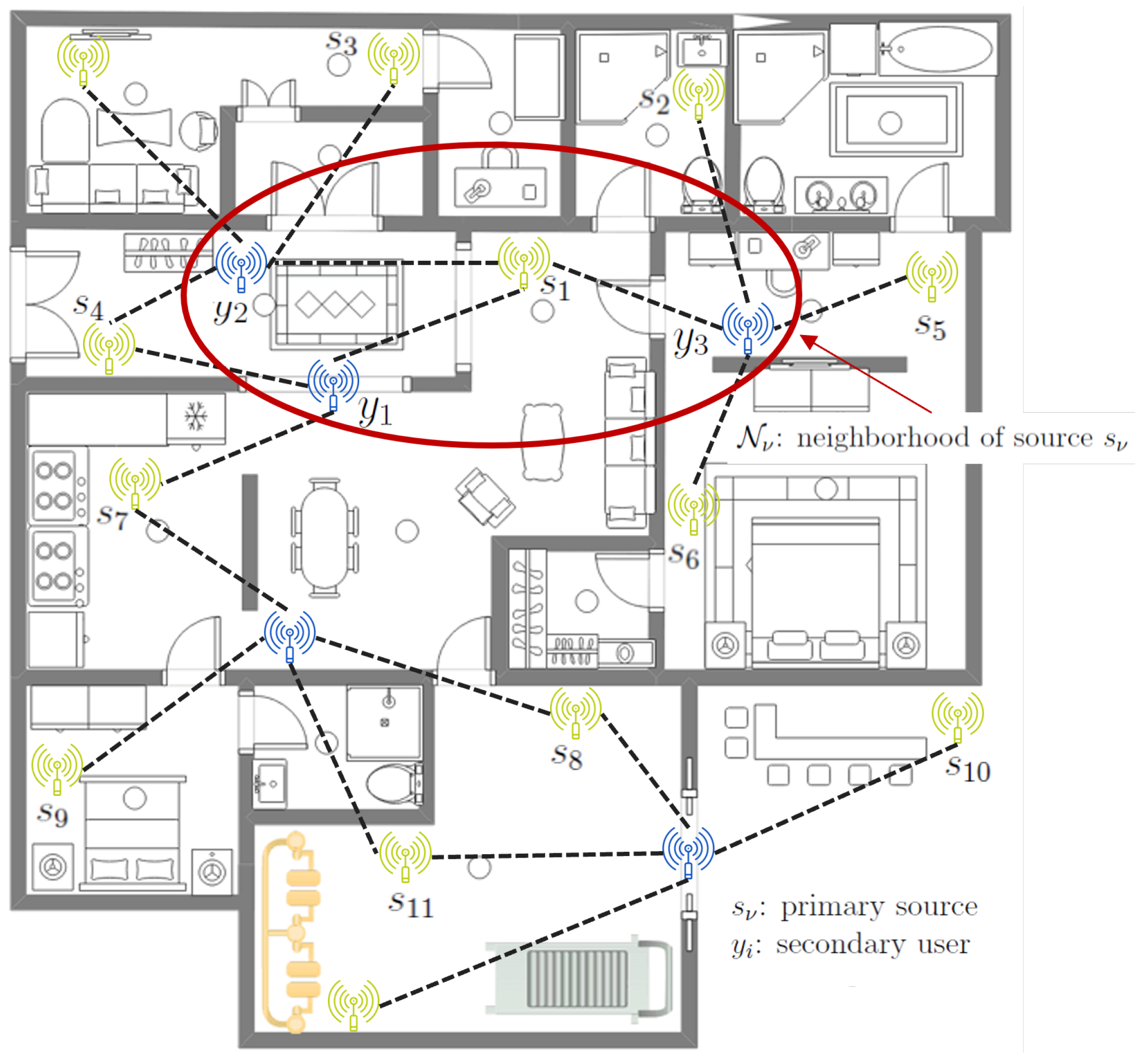
Figure 1. A CR-enabled IoT network deployment in a smart home environment.
Telecom 04 00029 g001
Figure 2. The graphical model we used for establishing the network structure of an SU network. Shaded nodes distribute the messages of the respective source to all the neighbors connected with it. s μ ( h ^ μ ) and y i ( h i ) are the incoming messages to the primary source and secondary user, respectively. The network structure has been modeled as a Bethe lattice [49], where every secondary user/primary source is connected to an arbitrary number of primary sources/secondary users. We have assumed, without loss of generality, that the secondary user y i is the origin of the lattice and all the other sources are arranged in shells around this root node.
Telecom 04 00029 g002
Figure 3. Q ( H ) and Q ^ ( H ^ ) distributions of populations (fields) H and H ^ , respectively, for β and resolution K = 1000 . The criterion we used for the population dynamics algorithm to stop was to examine whether there were no fluctuations in these two fields after a specific number of iterations. In practice, the algorithm converges fast enough, always as a function of the resolution K. Obviously, there is a trade-off between accuracy and convergence speed.
Telecom 04 00029 g003
Figure 4. (a) Error detection rate as a function of the SNR for the message-passing algorithm and the population dynamics method in a random network. The network structure for testing these two algorithms consisted of 10 primary sources and 10 SUs with a random degree of connectivity between them. As can be seen, both algorithms exhibit similar performance. It is worth highlighting the fact that the small difference between these two curves at high SNR values lies in the presence of loops in the tree structure that we have assumed. (b) Convergence of the message-passing algorithm in random networks with various connectivity matrices for fixed SNR = 0 dB. The algorithm scales linearly with the number of sources (in this tentative simulation, equal to n t = 12 ) which, as expected, converges in the same number of iterations. The convergence depends only on the number of sources per sensor and not on the size of the neighborhood matrix, as can be seen. The error detection rate is fixed after a specific number of iterations, simplifying the complexity of the proposed algorithm.
Telecom 04 00029 g004
Figure 5. (a) A single instantiation of a 20 × 20 random network. (b) Error detection rate for the network of (a). The red line represents the performance of myopic SU and the blue line represents the population dynamics algorithm. Note that above 0 dB, the proposed algorithm based on belief propagation outperforms the simple case of single-source detection.
Telecom 04 00029 g005
Figure 6. Performance comparison of the population dynamics algorithm and belief propagation algorithm, applied in 200 different random networks, all in an area A of 5 m 2 . The network consists of (a) 5 sources and 5 sensors, and (b) 10 sources and 10 sensors, all randomly connected to each other, and both path loss and Rayleigh fading have been considered.
Telecom 04 00029 g006
Figure 7. Error detection rate as a function of sources’ T and SUs’ R factors for fixed SNR = 0 dB. The network consists of 10 sources and 10 SUs, and the SUs’ and sources’ densities range from 0.1 to 1. (a) The error detection rate P err derived from the population dynamics algorithm according to (37), and (b) the total error detection rate P tot , which includes the probability of a node to be isolated. We have assumed that r c = 0.5 and the environmental factor γ = 4 . The regions (between contours) with the same colors have the same error detection rate (in dB). As expected, since R and T are proportional to densities n s and n t , the total error detection rate becomes higher when the number of SUs placed within the area of an emitting source is small.
Telecom 04 00029 g007
Table 1. Comparison of belief propagation with state-of-the-art methods in the detection of a source operational state.
Thresholding-based methods compare the received signal strength or other relevant parameters with a predefined threshold to infer the emitting state of the primary sources [24,25,26]. In summary, thresholding-based methods offer simplicity and speed but they may lack adaptability and robustness to complex data distributions. Belief propagation, on the other hand, provides adaptability, accuracy, and flexibility but has higher computational complexity and potential convergence challenges.
Advantages Compared to the Belief Propagation Algorithm
  • Lower complexity, since they are straightforward and easy to implement, thus they are more computationally efficient.
  • Rapid decision making, since they do not require extensive computations or iterations.
  • Robustness to noise and fluctuations that affect the emitting state detection by setting appropriate thresholds.
Drawbacks Compared to the Belief Propagation Algorithm
  • Lack of adaptability, since they rely on fixed thresholds, which may not capture the full complexity of the data distribution and thus can lead to suboptimal results.
  • Sensitivity to threshold selection, since they heavily rely on choosing appropriate thresholds. Selecting thresholds that are too low or too high can lead to false positives or false negatives, respectively, impacting the accuracy of the emitting state detection.
  • Lack of incorporation of prior knowledge, which in many cases, is crucial for the improvement of the accuracy of the emitting state detection.
  • Lack of iterative refinement, which hinders gradual improvement in the accuracy of the emitting state detection.
Statistical techniques, such as cumulative sum (CUSUM) or exponentially weighted moving average (EWMA), monitor sensor measurements over time and detect significant changes or deviations from the baseline [27,28,29,30,31]. In summary, statistical techniques are straightforward to implement, provide quick responses to state changes, and are computationally efficient. However, they may struggle to differentiate subtle changes, are prone to false alarms, and lack adaptability to changing environments. On the other hand, belief propagation offers more sophisticated modeling capabilities and can capture contextual information, temporal dependencies, and inter-sensor relationships. It provides higher discriminative power but has higher computational complexity. It may require more computational resources, but it can provide more precise and reliable emitting state detection, especially in complex scenarios.
Advantages Compared to the Belief Propagation Algorithm
  • Simplicity, since they typically involve analyzing the deviations or changes in the sensor measurements, making them easier to grasp and implement compared to more complex algorithms.
  • Real-time detection, since they respond fast to changes in sensor readings, making them particularly effective in situations where immediate action is required.
  • Minimal computational requirements, since they rely on simple statistical calculations or thresholding, making them computationally efficient for real-time applications or resource-constrained environments.
Drawbacks Compared to the Belief Propagation Algorithm
  • Lack of contextual information, since they typically focus on identifying abrupt changes in sensor readings without considering the underlying contextual information or relationships between sensors. This limitation can lead to false positives or false negatives, especially in complex scenarios where sensor data are interrelated.
  • Limited discriminative power, since they may struggle to differentiate between subtle changes in sensor readings or accurately distinguish between different states. This limitation can result in less precise or less reliable sensor state detection.
  • Sensitivity to noise and variability, since they are more susceptible to noise, outliers, or variations in sensor readings. Slight fluctuations or noise in measurements may trigger false alarms or affect the accuracy of state detection, especially when dealing with noisy or unreliable sensor data.
  • Lack of adaptability, since they often rely on predefined thresholds or statistical models that assume stationary or known distributions. They may struggle to adapt to changing environments or evolving sensor characteristics, limiting their robustness and adaptability.
Hidden Markov Models (HMMs), which are widely employed for modeling and detecting the state of sensors, are able to capture the temporal dependencies and transitions between different sensor states. They can infer the most likely sequence of sensor states by analyzing the sequence of observations [32,33,34]. In summary, HMMs excel in capturing temporal dependencies and modeling sequential data, making them suitable for time-series analysis. On the other hand, BP offers flexibility and can be applied to various graphical models, enabling distributed computations and scalable inference. While HMMs assume Markovian processes and have computationally intensive training, BP is more adaptable, but it is sensitive to model structure and may require approximations in loopy graphs.
Advantages Compared to the Belief Propagation Algorithm
  • Temporal modeling, since HMMs are well-suited for capturing temporal dependencies and modeling sequential data, as they can effectively model the transitions between different states over time, making them advantageous for applications where temporal dynamics are crucial.
  • Probabilistic inference, which provides a probabilistic framework for state estimation. HMMs explicitly model the probability distributions of observations and state transitions, enabling principled probabilistic inference and decision making.
  • Handling partial observations, since HMMs can handle scenarios where only partial observations are available. By using well-known algorithms, such as the forward-backward algorithm, they can estimate the most likely sequence of hidden states, even when some observations are missing or incomplete.
Drawbacks Compared to the Belief Propagation Algorithm
  • Strong assumptions, since they assume that the system being modeled follows a Markov process with discrete states and that observations are conditionally independent given the hidden states. These assumptions may limit their applicability in scenarios where the underlying system does not conform to these assumptions.
  • Lack of scalability, since the computational complexity of HMMs increases exponentially with the number of hidden states and observations. This can make training and inference computationally intensive, particularly for large-scale problems with a large number of states or observations.
  • Lack of flexibility and generalization, since they are limited to specific assumptions about the system or the data.
  • Lack of distributed computations, since HMMs are typically formulated as centralized models, where the inference and learning processes are performed on a single machine or system. Variations and extensions of HMMs have been proposed to enable distributed computations in certain scenarios, but they raise the overall complexity of the detection process.
Table 2. Transformation between bipolar and binary representations.
BinaryBipolarTransformation
s { 0 , 1 } s ¯ { 1 , 1 } s ¯ = 2 s 1
y = G s + η y ¯ = ( 2 G ) s ¯ + η y ¯ = y + G 1
min x y Gs min s ¯ y ¯ ( 2 G ) s ¯
s.t    s { 0 , 1 } N s.t    s ¯ { 1 , 1 } N
Table 3. Analogies of probability theory with statistical mechanics and the respective terms used in this paper.
ProbabilityStatistical MechanicsStatistical Mechanics Terminology
ln P ( y | s ) P ( s ) β E ( s | y ) Energy Functional
P ( y ) = s P ( y | s ) P ( s ) Z = s exp β E ( s | y ) Partition Function
P ( s | y ) Z 1 exp β E ( s | y ) Gibbs Probability of State s
argmax s P ( s | y ) argmax s E ( s | y ) = lim β 1 β ln Z Ground State
ln P ( y ) F = 1 β ln Z Gibbs Free Energy
Table 4. Parameter settings for the obtained simulations.
ParameterValue
Path Loss Exponent γ = 4
Communication Range r c
Average Density of Sources n t
Average Density of SUs n s
Source Activity Probability P α = 0.5
Disclaimer/Publisher’s Note: The statements, opinions and data contained in all publications are solely those of the individual author(s) and contributor(s) and not of MDPI and/or the editor(s). MDPI and/or the editor(s) disclaim responsibility for any injury to people or property resulting from any ideas, methods, instructions or products referred to in the content.