Optimal Adaptive Modeling of Hydrogen Polymer Electrolyte Membrane Fuel Cells Based on Meta-Heuristic Algorithms Considering the Membrane Aging Factor

Abstract

An efficient adaptive modeling criterion for the polymer electrolyte membrane fuel cell (PEMFC) is proposed in this paper, which can facilitate its precise simulation, design, analysis and control. In this work, a number of state-of-the-art algorithms have been adapted to optimize the complex electrochemical PEMFC model. Investigations are carried out not only from the conventional perspective of modeling accuracy but also from a new perspective represented by the impact of process computational time. Here, a novel technique of PEMFC modeling is proposed based on a meta-heuristic optimization algorithm called the wild horse optimizer (WHO). The proposed technique is concerned with the impact of the computational time on dynamic PEMFC modeling. A comprehensive statistical analysis was performed on the results of competing meta-heuristic optimizers that were adapted to a common PEMFC modeling problem. Among them, the proposed WHO approach’s results showed a promising performance in terms of its accuracy and minimum computational time over the other state-of-the-art approaches. For further evaluation of the WHO approach, it was used to optimize additional commercial PEMFC stack models. The results of the WHO approach highlighted its superior performance from the point of view of a high accuracy with a low computational burden, which supports its suitability for online applications.

1. Introduction

In the last few years, researchers and engineers have paid more attention to the development of hydrogen fuel cells. As promising clean energy conversion devices, they can provide creative solutions for the development of sustainable energy systems. Among all types of fuel cells, the polymer electrolyte membrane fuel cell (PEMFC) is considered the race horse on the track due to the following advantages: eco-friendliness (the only by-product is water vapor), low operating temperature (70–85 °C), so a shorter start-up time, high efficiency (50–70%), high current intensity, robustness, ability to operate at different humidity levels and modular design [1,2,3,4,5,6]. Because of these advantages, PEMFCs have become a reputable and integral part of many power system solutions in applications such as space crafts, electromotive applications and stationary renewable energy systems [7]. Like any technology, PEMFCs have some drawbacks; the main one is membrane deterioration, which affects its lifetime. Many studies have been proposed to elongate PEMFCs’ lifetimes by slowing down the membrane deterioration process [8]. A PEMFC’s performance/characteristics depend on its age as the catalyst is subjected to dissolution and the electrodes are subjected to wearing. The membrane deterioration process can be slowed by avoiding cold starts, multiple runs and the effects of sudden load changes [9,10]. The aforementioned conditions make PEMFC modeling a challenging process and necessitate the development of adaptive models that are able to mimic a PEMFC’s performance throughout its lifetime. An adaptive model helps to ensure the accurate operation of PEMFCs by selecting the proper operating conditions and supports its ability to satisfy the load demand in safe conditions [11,12]. Great efforts have been made to develop efficient PEMFC models to simulate the cells’ characteristics. The models can be classified into the following categories: (A) PEMFC physical models: they are developed based on the properties of the internal construction materials, which is useful for the testing and development phases. (B) PEMFC empirical models: they are developed based on large amounts of experimental data and intelligent algorithms, but they give no consideration to the physical characteristics of the cell, and require significant efforts to collect data and maintain the system’s computational capabilities. (C) PEMFC quasi-empirical models: they are developed based on experimental data and physical knowledge; they excel due to the combination of the good features of the two previous techniques [13]. The polarization curve, or the voltage –current (V-I) one, which is characteristic of quasi-empirical models, utilizes operating factors like the pressures and flow rates of hydrogen, oxygen and water inside the membrane and the operating temperature of the cell. The advantages of this model have qualified it to be the focus of many studies on topics including PEMFC system design, optimization and analysis [14,15,16].

The PEMFC quasi-empirical models are known as multi-variable nonlinear systems, which present complex problems when identifying the accurate values of the model’s parameters [17]. The conventional deterministic methods are not suitable for dealing with such problems; however, meta-heuristic methods have shown a proven performance in this regard. A lot of studies have shown the effective performance of meta-heuristic algorithms in solving complicated engineering problems such as design, simulation and modeling. Plus, thanks to their flexibility in adapting to problems, meta-heuristic algorithms have no restrictions in terms of problem formulation and are free of derivatives. That is why many recently developed meta-heuristic algorithms have been implemented in fuel cell modeling studies. As a result of the continuous development of algorithms, the door is still open for new algorithms inspired by biological, physical and natural phenomena to be implemented to improve and optimize PEMFC modelling [17,18,19]. The first attempts to extract the parameters of the PEMFC quasi-empirical model utilized the genetic algorithm (GA) and its modifications, as described in [20,21,22,23]. Despite the reasonable results obtained in these previous studies, it is remarkable that the GA’s results showed the undesirable feature of premature convergence. Subsequent studies proposed particle swarm optimization (PSO) as a more effective method for developing an accurate PEMFC model, as in [24]. The enhanced performance of PSO in dealing with the PEMFC modeling problem encouraged researchers to adapt other methods like differential evolution (DE) and its hybridization [25,26,27]. The most recent methods succeeded in obtaining more accurate parameters in the search for efficient PEMFC models. This problem was approached using the harmony search algorithm (HAS) with flexible implementation and showed good results in terms of accuracy [28]. Consequently, a novel P-system-based method (BIPOA) [29] and teaching–learning-based optimization (TLBO) [30,31] were adapted to improve the PEMFC model’s accuracy for different fuel cell devices. After that, the PEMFC parameter was efficiently identified by utilizing a hybrid stochastic strategy based on the selectivity feature as described in [32]. The gray wolf algorithm also showed a reputable performance in the PEMFC modeling of commercial devices based on actual measured data [19]. In [33], the salp swarm optimizer was implemented to deal with parameter extraction for the PEMFC model to enhance the fit between the estimated model curve and the experimental data. A bio-inspired algorithm shark smell optimizer showed an effective performance in identifying the PEMFC model parameters as illustrated in [34]. Later, the authors of [35] utilized an improved fluid search algorithm and formulated the problem based on the summation of squared errors (SSEs) to extract more accurate PEMFC model parameters. In the same vein, the problem was approached using the marine predator optimization algorithm and the parameters extracted showed the ability of the technique, as shown in [36]. Recently, a new algorithm called coot bird optimizer was utilized to adaptively develop PEMFC models along its lifetime with regard to computational burden [37].

From the above survey, it can be concluded that the majority of PEMFC modeling studies have given priority to estimating the most accurate model parameters. Fewer studies have paid attention to adaptive models and the impact of computational burden. The computational burden factor is important to certify the suitability of the technique for developing adaptive models, which can be implemented in real-time applications to mimic the PEMFC model’s characteristics throughout its life. Adaptive models help in the proper control of the cell by using updated polarization curves and support the cell efficiency. The concept of the no-free-lunch theory revolves around the fact that no method fits all optimization problems in various conditions [38]. These details were the impetus to conduct this study and propose a novel solution method that combines solution accuracy, computational time reduction and simplicity of implementation. These features are essential to suit the requirements of the online application of the PEMFC model. In this context, the proposed method was investigated through the utilization of actual data from commercial PEMFC devices. In addition, comprehensive comparisons and statistical analyses were performed to evaluate the proposed method in comparison with other competitors.

The main contributions of this work can be summarized as follows:

• A novel adaptive meta-heuristic WHO-based method for PEMFC modeling is proposed.
• A fair comparison of state-of-the-art algorithms dealing with typical PEMFC modeling problems is performed.
• The modeling accuracy and the impact of computational time are used as critical factors for evaluation.
• The robustness of the proposed approach is validated through the implementation of commercial PEMFC devices named 250 W PEMFC, Nedstack-PS6 6 kW, Temasek 1 kW, Ballard-Mark-V 5 kW.
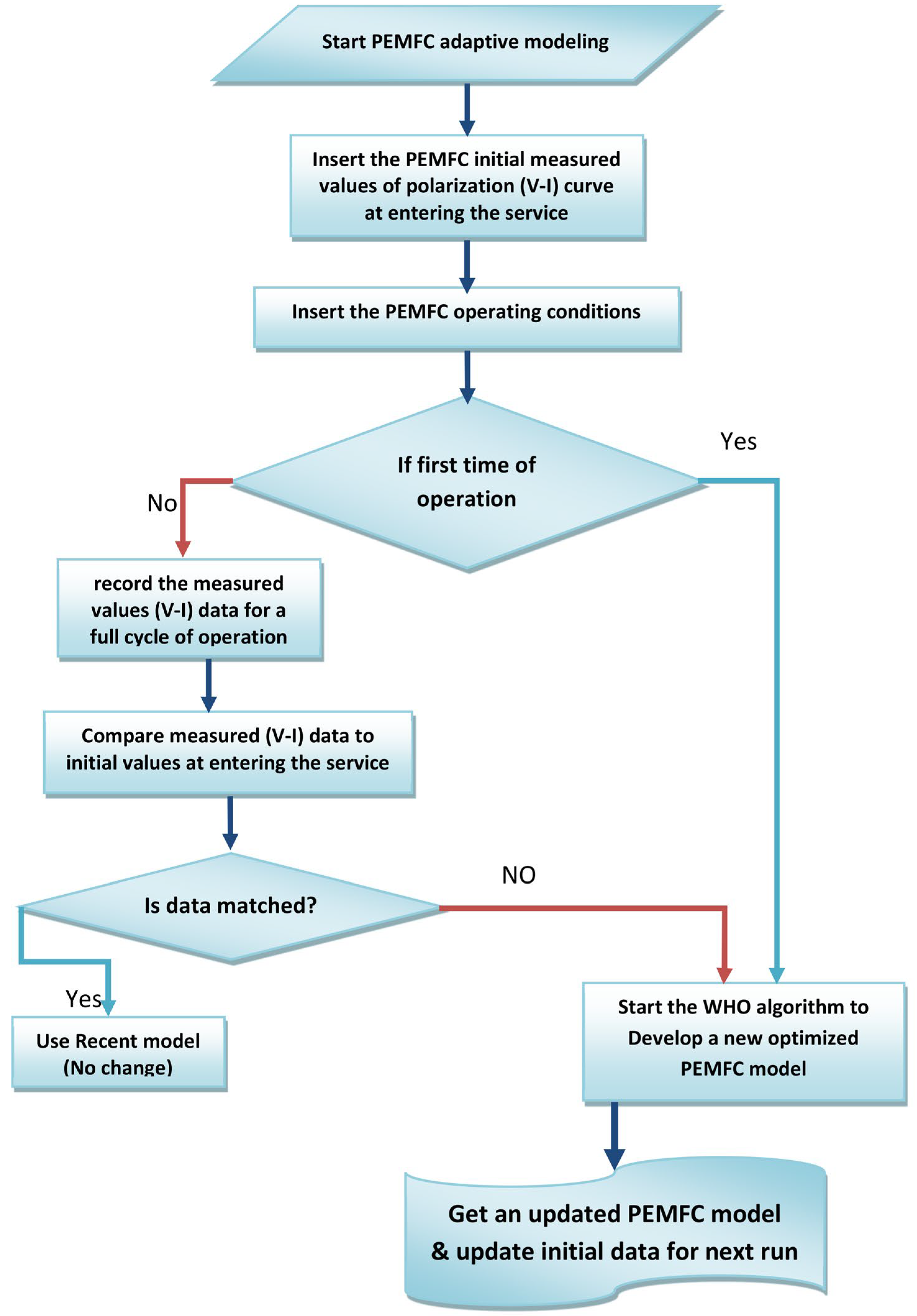
• The accurate adaptive characterization of PEMFC is capable of reflecting dynamic changes in the cell’s performance in accordance with aging behavior.

2. Theoretical Approach

2.1. Description of the PEMFC Model

2.1.1. PEMFC Notion

PEMFC is an electrochemical device that efficiently converts chemical energy to electrical energy according to its internal reactions. The cell consists of two catalyst-coated electrodes (anode and cathode) and a solid polymer electrolyte is placed between the electrodes as shown in Figure 1. From the figure, it is clear that the hydrogen is fed through the anode inlets to reach the surface of the catalytic material of the electrode, which activates the membrane reaction. The reaction starts by splitting the hydrogen into protons which migrate across the membrane to reach the cathode and electrons which flow in the electrical external circuit. The oxygen atoms are fed through cathode inlet units with the migrated hydrogen protons to form water molecules [1,2,19,37].

The membrane chemical reaction can be represented by the following:

$$H_2+{\displaystyle \frac{1}{2}}{O}_2\to H_{2}O+Energy$$

(1)

In Equation (1), the term energy refers to the output electricity produced by the cell.

2.1.2. PEMFC Quasi-Empirical Model

The well-known Amphlett et al. [5] formulation of the PEMFC model is utilized in this study, taking into consideration the improvements in [1,17,27]. As such, the PEMFC output voltage ($V_{FC}$) is expressed by the following equation:

$$V_{FC}=N_{Cells}\ast (E_{Nernst}-V_{Act}-V_{Ohmic}-V_{Conc})$$

(2)

where $N_{Cells}$ is the number of a PEMFC stack cells, $E_{Nernst}$ represents the PEMFC theoretical voltage known as the Nernst voltage given by Equation (3), while the terms $V_{Act}$ (the cell activation loss due to reaction initiation at membrane electrodes), $V_{Ohmic}$ (the cell Ohmic loss due to membrane and terminal resistance) and ${ V}_{Conc}$ (the concentration loss that represents transfer loss due to an increase in proton migration through the membrane), respectively, represent the internal voltage losses that happen throughout the cell, as illustrated in Figure 2a,b.

The PEMFC theoretical voltage $E_{Nernst}$ is given by the following:

$$\begin{gathered} E_{Nernst}=1.229-0.85\times {10}^{-3}\left(T-298.15\right) \\ +4.3085\times {10}^{-5}\times T\times ln\left({\displaystyle \frac{p_{H_2}^1{p}_{O_2}^{0.5}}{p_{H_{2}O}}}\right) \end{gathered}$$

(3)

where $T$ is the cell operating temperature in Kelvin, while $p_{H_2}$ and $p_{O_2}$ are the hydrogen and oxygen partial pressures through the membrane, respectively, in kPa ($atm$) given by Equations (4) and (5); $p_{H_{2}O}$expresses the membrane saturation pressure in kPa ($atm$) given by Equation (6) [5,15].

$$p_{H_2}=0.5({RH}_a\times p_{H_{2}O})\left[{\left({\displaystyle \frac{{RH}_a\ast p_{H_{2}O}}{p_a}} e^{{\displaystyle \frac{1.635\left(\raisebox{1ex}{$I_{FC}$}\!\left/ \!\raisebox{-1ex}{$A$}\right.\right)}{T^{1.334}}}}\right)}^{-1}-1\right]$$

(4)

$$p_{O_2}=({RH}_c\times p_{H_{2}O})\left[{\left({\displaystyle \frac{{RH}_c\ast p_{H_{2}O}}{p_c}} e^{{\displaystyle \frac{4.192\left(\raisebox{1ex}{$I_{FC}$}\!\left/ \!\raisebox{-1ex}{$A$}\right.\right)}{T^{1.334}}}}\right)}^{-1}-1\right]$$

(5)

$$\begin{gathered} p_{H_{2}O}=2.95\times {10}^{-2}\left(T-273.15\right)-9.18\times {10}^{-5}{\left(T-273.15\right)}^2 \\ +1.44\times {10}^{-7}{(T-273.15)}^3-2.18 \end{gathered}$$

(6)

where $I_{FC}$ is the PEMFC output current in $\mathrm{A}\mathrm{m}\mathrm{p}\mathrm{e}\mathrm{r}\mathrm{e}\mathrm{s}$ (A); ${RH}_a$ and ${RH}_c$ are the relative humidity at the electrodes, respectively; $p_a$ and $p_c$ are the anode and cathode inlet pressures, respectively, in kPa ($atm$); and $A$ is the effective area of the membrane in ${\mathrm{c}\mathrm{m}}^2$.

The aforementioned activation loss $V_{Act}$ due to the initiation of the cell chemical reaction is computed by

$$V_{Act}=-({\xi }_1+{\xi }_2\times T+{\xi }_3\times T\times \mathrm{l}\mathrm{n}(C_{O_2})+{\xi }_4\times T\times \mathrm{l}\mathrm{n}(I_{FC}\left)\right)$$

(7)

where ${\xi }_1$, ${\xi }_2$, ${\xi }_3$, ${\xi }_4$ are unknown parameters of the model that need to be identified next for certain types of PEMFCs. The term $C_{O_2}$ represents the electrode’s oxygen concentration in $\mathrm{m}\mathrm{o}\mathrm{l}/{\mathrm{c}\mathrm{m}}^3$, given by (8) [20,27].

$$C_{O_2}={\displaystyle \frac{p_{O_2}}{5.08\times {10}^6\times e^{-498/T}}}$$

(8)

The Ohmic voltage loss $V_{Ohmic}$ depends on the internal membrane resistance $R_m$ and the interface connection resistance $R_c$ which can be calculated by

$$V_{Ohmic}=I_{FC}(R_m+R_c)$$

(9)

where the first part $R_m$ is a variable that depends on the hydration level of the membrane medium, and the second part $R_c$ is fixed and occurs due to contact issues at the electrode terminals, all in $\mathrm{O}\mathrm{h}\mathrm{m}$, and $R_m$ is given by

$$R_m={\displaystyle \frac{{\rho }_{m}l}{A}}$$

(10)

While $l is$ the cell membrane thickness in $\mathrm{c}\mathrm{m}$, and ${\rho }_m$is the specific resistance of the cell membrane in Ohm centimeters ($\mathsf{\Omega }\mathrm{c}\mathrm{m}$), which can be computed by

$${\rho }_m={\displaystyle \frac{181.6\times \left[1+0.03\left(\frac{I_{FC}}{A}\right)+0.062{\left(\frac{T}{303}\right)}^2{\left(\frac{I_{FC}}{A}\right)}^{2.5}\right]}{\left[\Psi -0.634-3\left(\frac{I_{FC}}{A}\right)\right]e^{\frac{4.18(T-303)}{T}}}}$$

(11)

The specific resistance relies on the membrane hydration level parameter $\Psi$ (which is a variable that takes the values from 10 to 24), the cell temperature and the current density $\left({\displaystyle \frac{I_{FC}}{A}}\right)$ [19,27].

The concentration loss $V_{Conc}$ is calculated by

$$V_{Conc}=-B.ln\left(1-{\displaystyle \frac{i_d}{i_L}}\right)$$

(12)

where $i_d$ is the density of protons transfer across the membrane in ${\mathrm{m}\mathrm{A}\mathrm{c}\mathrm{m}}^{-2}$ and $B$ is an unknown coefficient in $Volt$. As a result of the increase in the load demand current, the migrating protons’ density increases across the membrane to meet the limit of saturation. At this limit the concentration loss spikes to critical values that make the output voltage collapse as shown in Figure 2. According to experimental measurements, the maximum limit of the current density $i_L$ in ${\mathrm{m}\mathrm{A}\mathrm{c}\mathrm{m}}^{-2}$ can be estimated to avoid the inefficient operation of the cell [1,19].

Subsequently, Equations (2)–(12) represent the quasi-empirical model which mimics the characteristics of the PEMFC. The unknown parameters (${\xi }_1, {\xi }_2, {\xi }_3, {\xi }_4, \Psi ,R_c,B$) of the mathematical equation system must be accurately identified to finish the model and produce a polarization curve for the PEMFC device.

2.2. WHO Algorithm

The WHO algorithm is a recently developed meta-heuristic algorithm. It is designed to mimic the amazing biological behavior of wild horses. Wild horses live in groups in nature; each group consists of a stallion, mares, foals and offspring. The group behavior comprises grazing, leading, governing, pursuing and mating [39,40]. A brief illustration of the coding and mechanisms of WHO is described in the following subsections.

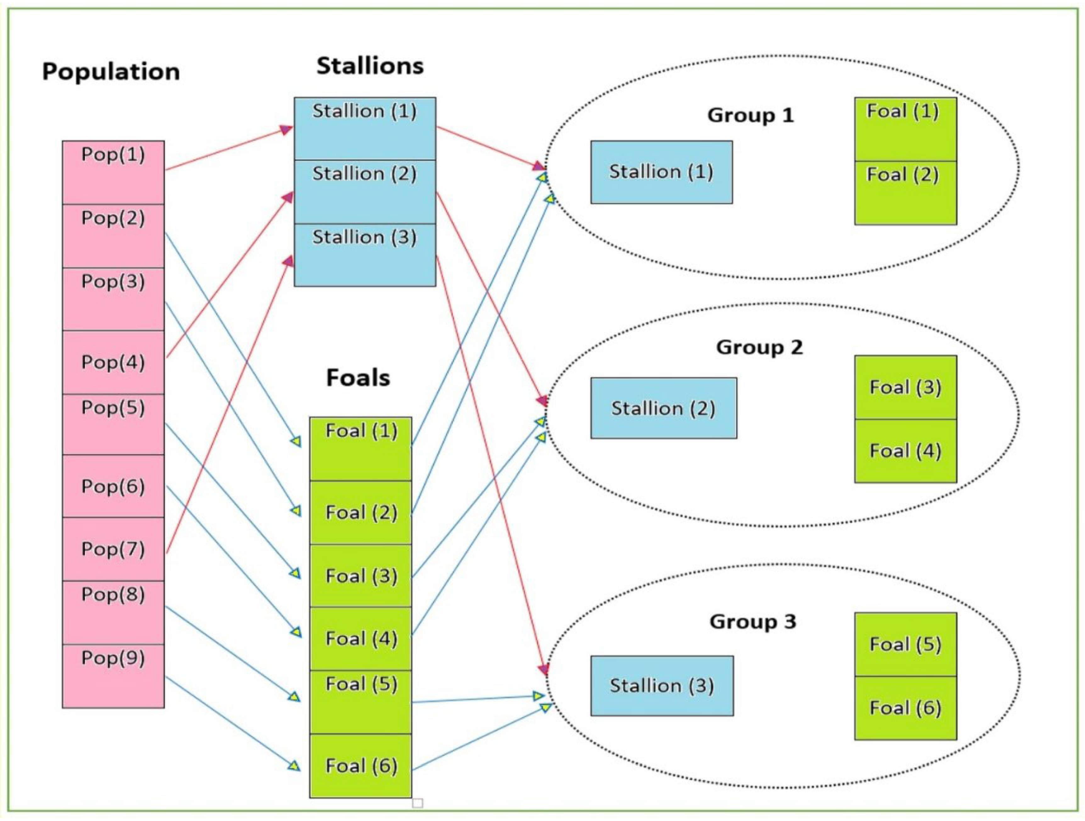
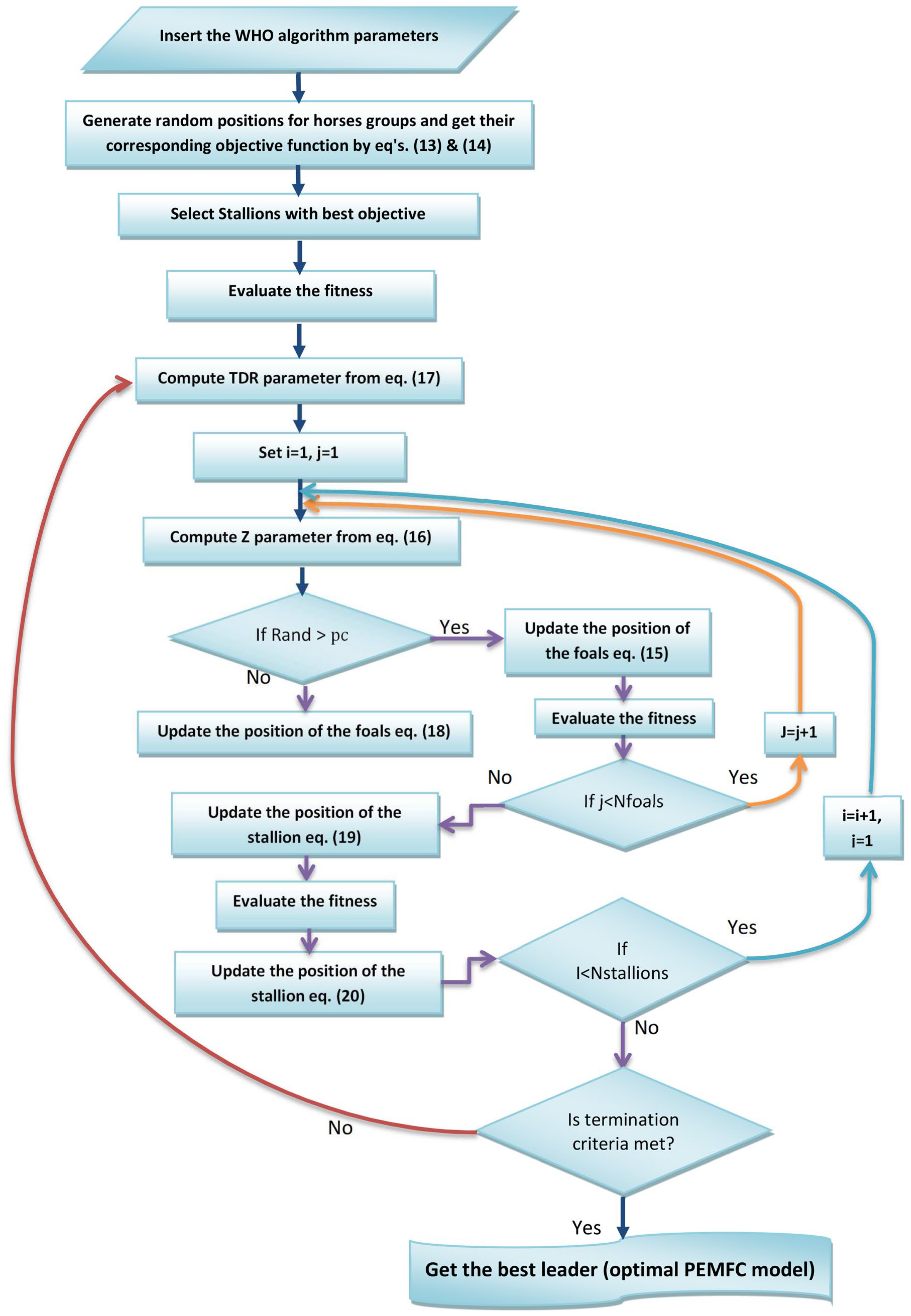
2.2.1. The WHO Mechanism

Using the aforementioned behaviors, the algorithm mechanism is configured to simulate the manners of grazing, mating, leadership and governing [41]. These behaviors are translated to five mechanisms, as listed below:

• Start with an initial population that simulates horse groups and nominate a leader.
• Simulate grazing and mating behaviors.
• One stallion becomes the leader of the group.
• The group select and replace each new leader with a better leader.
• The best leader is found (the solution).

Starting the Initial Population

Similar to any optimization algorithm, the WHO randomly creates its first population of horses as shown in Equation (13) and its corresponding objective function is calculated as shown in Equation (14). A repetitive iterations process is performed to enhance the objective results of horses.

$$X=\{X_1, X_2, X_3, \dots \dots \dots , X_n\}$$

(13)

$$O=\{O_1, \mathrm{O}, O_3, \dots \dots \dots , O_n\}$$

(14)

The wild horses are sectioned into groups where $n$ represents the number of horses within population and $G$ represents the number of group leaders (stallions) given as $G=n\times ps$, where $ps$ is the percentage of leaders out of the total population. The stallion leads his group, so the number of stallions equals the number of groups. The rest of the population is considered to be mares and foals, as described in Figure 3.

The Grazing Simulation Mechanism

The algorithm in this stage mimics the behavior of wild horses moving and exploring around their leader in nature. The position of a group of horses can be defined according to the following equation:

$${\overline{X}}_{i,G}^j=2\mathrm{Z}\cos \left(2\pi RZ\right)\times \left({Stallion}^j-X_{i,G}^j\right)+{Stallion}^j$$

(15)

where the symbol $\mathrm{Z}$ is an adaptive parameter given by Equation (16), ${Stallion}^j$ is the current position of the leader, $R$ is a random value between [−2, 2] that scatter the horses around their stallion in 360 degrees and $X_{i,G}^j$ represents the current position of the group that should be updated.

$$P={\stackrel{⃑}{R}}_1<\mathrm{T}\mathrm{D}\mathrm{R};IDX=\left(\mathrm{P}==0\right);\mathrm{Z}=R_2\mathsf{\Theta }IDX+{\stackrel{⃑}{R}}_3\mathsf{\Theta }\left(~IDX\right)$$

(16)

where $P$ represents a vector with the same dimension of the problem formed from zeros and ones, TDR is a descending parameter which starts at a value of 1 and reaches 0 after the max number of iterations, which is given by Equation (17), the symbol $R_2$ is a random parameter uniformly distributed in the range of 0 to 1, ${\stackrel{⃑}{R}}_1$ and ${\stackrel{⃑}{R}}_3$ are vectors and $IDX$ is an index for vector ${\stackrel{⃑}{R}}_1$.

$$\mathrm{T}\mathrm{D}\mathrm{R}=1-Iter\times \left({\displaystyle \frac{1}{MaxIter}}\right)$$

(17)

where the symbol $Iter$ represents the most recent iteration number and $MaxIter$ represents the end of the iterative process.

The Mating Mechanism

One of the unique features of wild horses is their manner of mating, as the foals depart the group to prevent fathers from mating with their daughters. This manner of mating is simulated by assuming that foals transfer between three groups called I, j and k. The position of a horse transferred from group k can be calculated by

$$X_{G,k}^p=\mathrm{C}\mathrm{r}\mathrm{o}\mathrm{s}\mathrm{s}\mathrm{o}\mathrm{v}\mathrm{e}\mathrm{r}\left(X_{G,i}^q,X_{G,j}^z\right) i\ne j\ne k, p=q=end, \mathrm{C}\mathrm{r}\mathrm{o}\mathrm{s}\mathrm{s}\mathrm{o}\mathrm{v}\mathrm{e}\mathrm{r}=\mathrm{M}\mathrm{e}\mathrm{a}\mathrm{n}$$

(18)

where $X_{G,i}^q$ and $X_{G,j}^z$ are the positions at which q and z horses departed from the i and j groups, respectively.

Selecting the Leader Mechanism

The leader’s main role is to direct the group to a desired place which contains water holes. Different group leaders compete to find the water hole and the governing group possesses it and prevents other groups from using it. This possession remains until another group gains the power to govern this water hole and possess it. The following equation simulates this by finding the new position of governing stallion ${\overline{Stallion}}_{G_i}$ from group i as

$${\overline{Stallion}}_{G_i}=\left\{\begin{array}{c}2Z\cos \left(2\pi RZ\right)\times \left(WH-{Stallion}_{G_i}\right)+WH if R_{3 }>0.5 \\ 2Z\cos \left(2\pi RZ\right)\times \left(WH-{Stallion}_{G_i}\right)-WH if R_{3 }\le 0.5\end{array}\right.$$

(19)

where $WH$ represents the water hole position and ${Stallion}_{G_i}$ refers to the stallion’s most recent position.

The positions of stallions are updated to replace weak stallions with more fit stallions with better leadership properties. The position update mechanism is simulated by

$${Stallion}_{G_i}=\left\{\begin{array}{c}{X}_{G,i} if\cos t\left(X_{G,i}\right)<\cos t\left({Stallion}_{G_i}\right) \\ {Stallion}_{G_i} if\cos t\left(X_{G,i}\right)>\cos t\left({Stallion}_{G_i}\right)\end{array}\right\}$$

(20)

The flow chart which is depicted in Figure 4 describes the entire mechanism of the WHO algorithm.

2.3. Creating the Objective Function

The main target of this study is to propose an adaptive modeling criterion for PEMFC devices, which comprises their efficiency, flexibility and minimum computational burden. These features can qualify the method to be feasible for online applications through the efficient simulation of the practical PEMFC model’s performance. This study’s main goal is to develop an adaptive model of a PEMFC with a more enhanced accuracy in order to mimic the real performance of fuel cells in practical applications. For this purpose, the WHO is configured to optimize the problem of PEMFC modeling according to an objective function (SSE) represented by Equation (21). The objective function is built to minimize the summation of the squared errors (SSEs) between the actual characteristic (V-I) curve and the estimated model curve. The output of the optimization process is accurate parameters for the quasi-empirical PEMFC model (${\xi }_1, {\xi }_2, {\xi }_3, {\xi }_4, \Psi ,R_c,B$), as mentioned in Section 2.2.

$$Minimize \left(SSE=\sum _{j=1}^J{\left(V_{actual,j}-V_{mdl,j}\right)}^2\right)$$

(21)

where $V_{actual}$ represents the actual data for the PEMFC device’s output voltage, $V_{mdl}$ represents the developed model voltage data and $j$ expresses several data points. The objective function assesses the validity of the developed model (V-I) data in comparison of the actual device data. The developed model’s effectiveness depends on the accuracy of the extracted parameters, where they are limited by constraints to guide the algorithm in the search space as expressed by Equation (22). The most reputable ranges of the unknown parameters were borrowed from [19,27,37] in order to be implemented in this study as depicted in

Table 1. Unknown parameters’ boundaries.

Model Parameter	${\mathsf{\xi }}_1$	${\mathsf{\xi }}_2$	${\mathsf{\xi }}_3$	${\mathsf{\xi }}_4$	$\mathsf{\Psi }$	${\mathit{R}}_{\mathit{c}}$	$\mathit{B}$
Lower boundary	−1.1997	0.001	3.6 × 10−5	−2.6 × 10−4	10	0.0001	0.0136
Upper boundary	−0.8532	0.005	9.8 × 10−5	−9.54 × 10−5	24	0.0008	0.5

.

$$\left.\begin{array}{c}{\xi }_{1min}\le {\xi }_1\le {\xi }_{1max}\\ {\xi }_{2min}\le {\xi }_2\le {\xi }_{2max}\\ {\xi }_{3min}\le {\xi }_3\le {\xi }_{3max}\\ {\xi }_{4min}\le {\xi }_4\le {\xi }_{4max}\\ \begin{array}{c}{\Psi }_{min}\le \Psi \le {\Psi }_{max}\\ R_{cmin}\le R_c\le R_{cmax}\\ B_{min}\le B\le B_{max}\end{array}\end{array}\right\}$$

(22)

Modeling an efficient adaptive PEMFC throughout its lifetime is the main target. In this context, updating the PEMFC model online can reflect the real characteristics of the aged cell membrane. This can achieve the proper control and operation of the cell and elongates its lifetime by avoiding undesired control orders [12]. Hence, this work proposes an adaptive modeling method that efficiently updates the PEMFC model. The update mechanism in the method depends on measuring the PEMFC terminal voltage–current during a full cycle of operation; thereafter, the aggregated data set is compared to the original data on the characteristics of the cell to explore any variation in the cell performance. The result of this comparison activates/deactivates the method to develop an updated model. The merits of the proposed WHO algorithm-based method are flexibility, simplicity and a low computational burden, so it can reduce the need for costive high-capability control systems. The proposed method mechanism is depicted in the flowchart in Figure 5.

3. Cases Under Study

The dynamic changes that occur to the PEMFC devices necessitate the development of an efficient adaptive model. This type of modeling ensures proper mimicry of the cell’s characteristics and is valid for online applications. That is why many recent meta-heuristic optimizers have applied the proposed adaptive method to develop an efficient PEMFC model. For evaluation purposes, a benchmarking process was designed in two stages. The first one is to apply different reputable meta-heuristic algorithms to develop a model for a common benchmark 250 W PEMFC. The device’s specifications and operational data are listed in

Table 2. Specification of the 250W PEMFC (First stage) [20,21].

Stack Parameters		Operation Ranges
Number of cells in series  ${\mathit{N}}_{\mathit{C}\mathit{e}\mathit{l}\mathit{l}\mathit{s}}$	24	$\mathrm{Inlet} \mathrm{anode} \mathrm{pressure} p_a$	100–300 kPa (1–3 bar)
Cell’s active area A	$27 \times 10{-}^4 {\mathrm{m}}^2$ $(27 {\mathrm{c}\mathrm{m}}^2$)	$\mathrm{Inlet} \mathrm{cathode} \mathrm{pressure} p_c$	100–500 kPa (1–5 bar)
Nafion 115:5 mil l	127 × 10−6 m (127 μm)	Stack temperature T	353.15–343.15 K
$\mathbf{Maximum} \mathbf{current} \mathbf{density} {\mathit{i}}_{\mathit{L}}$	$86 {\mathrm{A}/\mathrm{m}}^2$ (860 $\mathrm{m}{\mathrm{A}/\mathrm{c}\mathrm{m}}^2$)	$\mathrm{Relative} \mathrm{humidity} \mathrm{in} \mathrm{anode} {RH}_a$	1
Rated power	$250 \mathrm{W}$	$\mathrm{Relative} \mathrm{humidity} \mathrm{in} \mathrm{cathode} {RH}_c$	1

. The meta-heuristic optimizers utilized at this stage are listed as follows: modified vector differential evolution (MTDE) [42], the coot bird optimization algorithm (CBO) [37], the particle swarm optimizer (PSO) [24], atom search optimization (ASO) [43], the dragonfly algorithm (DA) [44], the grasshopper optimization algorithm (GOA) [45], equilibrium optimizer (EO) [46], ant–lion optimizer (ALO) [47] and the wild Horse Optimizer (WHO) [39].

The mathematical equations for the aforementioned quasi-empirical model are in Section 2.1.2. and are configured in the benchmarking process. Considering the boundaries and limits of the unknown parameters listed in Table 1. The 250 W PEMFC is modeled under four different operating conditions with the measured data (inlets pressures and cell temperature) as listed below:

• Operating condition (Data set 1): 300/500 kPa (3/5 bar), 353.15 K;
• Operating condition (Data set 2): 100/100 kPa (1/1 bar), 343.15 K;
• Operating condition (Data set 3): 250/300 kPa (2.5/3 bar), 343.15 K;
• Operating condition (Data set 4): 150/150 kPa (1.5/1.5 bar, 343.15 K.

The output in this stage defines the best algorithms to be qualified for further assessment in the second stage. Herein, three commercial fuel cell devices with different ratings, namely Nedstack-PS6 6 kW, Temasek 1 kW, Ballard-Mark-V 5 kW, are utilized to be modeled according to the proposed method. The specifications and operational data of the devices are borrowed from [19,27,31], as shown in

Table 3. The specifications and operational data of the devices under study.

PEMFC Type	Nedstack-PS6 6 kW [15,33]	Temasek 1 kW [19,36]	Ballard-Mark-V 5 kW [19,36]
$\mathbf{Number} \mathbf{of} \mathbf{cells} {\mathit{N}}_{\mathit{C}\mathit{e}\mathit{l}\mathit{l}\mathit{s}}$	65	20	35
Cell’s active area  $A ({\mathbf{m}}^2$)	240 × 10−4 $(240 {\mathrm{c}\mathrm{m}}^2$)	150 × 10−4 $(150 {\mathrm{c}\mathrm{m}}^2$)	232 × 10−4 m2 ($232 {\mathrm{c}\mathrm{m}}^2$)
Nafion 115:5 mil l (m)	178 × 10−6 178 μm	51 × 10−6 51 μm	178 × 10−6 178 μm
Max current density ${\mathit{i}}_{\mathit{L}}$ (${\mathbf{A}/\mathbf{m}}^2$)	120 $1200 {\mathrm{m}\mathrm{A}/\mathrm{c}\mathrm{m}}^2$	150 $1500 {\mathrm{m}\mathrm{A}/\mathrm{c}\mathrm{m}}^2$	150 $1500 {\mathrm{m}\mathrm{A}/\mathrm{c}\mathrm{m}}^2$
Stack temperature T (K)	343	323	343
$\mathbf{Hydrogen} \mathbf{pressure} {\mathit{P}}_{{\mathit{H}}_2}$ (kPa)	49.03325–490.3325	49.03325	98.0665
Oxygen pressure ${\mathit{P}}_{{\mathit{O}}_2}$ (kPa)	49.03325–490.3325	49.03325	98.0665

in order.

4. Methodology and Results

The assessment procedure for the recently developed optimizers was carried out in the MATLAB environment, version R2020a (9.8.0.1323502) 64-bit [48], driven by an Intel^®® core™ i5-5200U CPU, 2.7 GHz, 6 GB RAM Laptop. During the first assessment stage, the nine optimizers were adapted to the test modeling problem of the 250 W PEMFC. The process was planned to include 100 individual runs for each optimizer with the same values of tuned parameters (population = 20 and iterations = 500 for individual run) to guarantee fairness. The results from the first stage were encouraging, as depicted in

Table 4. The comparative results of modeling 250 W PEMFC.

Method	Fitness (SSE)	Elapsed Time *	${\mathsf{\xi }}_1$	${\mathsf{\xi }}_2$	${\mathsf{\xi }}_3$	${\mathsf{\xi }}_4$	$\mathsf{\Psi }$	${\mathit{R}}_{\mathit{c}}$	$\mathit{B}$
WHO	0.7579489	0.3759676	−0.9508	0.003543705	9.80 × 10−5	−9.54 × 10−5	24	0.0001	0.0136
CBO	0.84042	0.38703	−0.8593	0.0032844	9.80 × 10−5	−9.54 × 10−5	24	0.0001	0.0136
EO	0.840419	0.42235	−0.8532	0.003267329	9.80 × 10−5	−9.54 × 10−5	24	0.0001	0.0136
GOA	1.0897	5.323141	−1.14622	0.00379843	8.06 × 10−5	−9.54 × 10−5	24	0.0001	0.0136
MTDE	1.1531	3.804542	−1.061	0.0038525	9.80 × 10−5	−9.54 × 10−5	24	0.0001	0.0136
DA	1.1655	33.249382	−0.8532	0.00326576	9.80 × 10−5	−9.54 × 10−5	24	0.0001	0.0136
ALO	1.1659	2.75704	−0.87109	0.00303416	8.16 × 10−5	−9.54 × 10−5	24	0.0001	0.0136
ASO	1.3483	0.727816	−1.00738	0.00318212	6.75 × 10−5	−9.54 × 10−5	23.72	0.0005574	0.014613
PSO	1.7193	8.954077	−1.1997	0.0042618	9.80 × 10−5	−9.54 × 10−5	24	0.0001	0.0136
VSDE [27]	1.0526	Not reported	−1.1921	3.199 × 10−3	3.79 × 10−5	1.870 × 10−4	22.81	1.202 × 10−4	0.02903
TLBO-DE [16]	7.2776	Not reported	−0.8532	2.6505 × 10−3	8.0016 × 10−5	−1.360 × 10−4	15.65	1.0000 × 10−4	0.0364
QPSO [19]	7.2776	Not reported	−0.8569	2.5665 × 10−3	7.2708 × 10−5	−1.303 × 10−4	13.54	3.9173 × 10−4	0.0299
ITHS [31]	7.5798	Not reported	−0.9228	2.7348 × 10−3	7.0967 × 10−5	−1.426 × 10−4	16.52	1.0091 × 10−4	0.0362
Sa-DE [31]	7.6276	Not reported	−0.8534	2.5846 × 10−3	7.5880 × 10−5	−1.154 × 10−4	12.6	1.0000 × 10−4	0.0329
STLBO [31]	7.6426	Not reported	−0.8532	2.5843	7.6892 × 10−5	−1.154 × 10−4	12.6	1.0000 × 10−4	0.0329
BIPOA [29]	7.9416	Not reported	−0.8016	2.6673 × 10−3	8.1288 × 10−5	−1.271 × 10−4	13.51	0.80	0.0324
ARNA-GA [23]	8.1039	Not reported	−0.8806	2.9450 × 10−3	8.4438 × 10−5	−1.288 × 10−4	13.48	1.0068 × 10−4	0.0316
RGA [21]	8.4854	Not reported	−1.1568	3.4243 × 10−3	6.4161 × 10−5	−1.154 × 10−4	12.89	1.4504 × 10−4	0.0343
MPSO [19]	9.7539	Not reported	−0.9479	3.0835 × 10−3	7.7990 × 10−5	−1.880 × 10−4	20.76	2.8666 × 10−4	0.0296

* Elapsed time: represents the average elapsed time in seconds.

along with other comparative findings from the literature.

The results of the algorithms’ bench marking processes are listed in Table 4, in comparison to the same problem reported in the literature under the same conditions. From this table, it can be seen that three optimizers (WHO, CBO and EO) achieved the top results in terms of accuracy (minimum SSE). This is an encouraging indication about the validity of these optimizers for this modeling process.

Further statistical and computational analyses were performed using the IBM-SPSS software (Version 22) [49], and the outcomes are depicted in

Table 5. Statistical and computational analysis of the comparative optimizers results.

Algorithm	PSO	MTDE	ALO	DA	ASO	GOA	EO	CBO	WHO
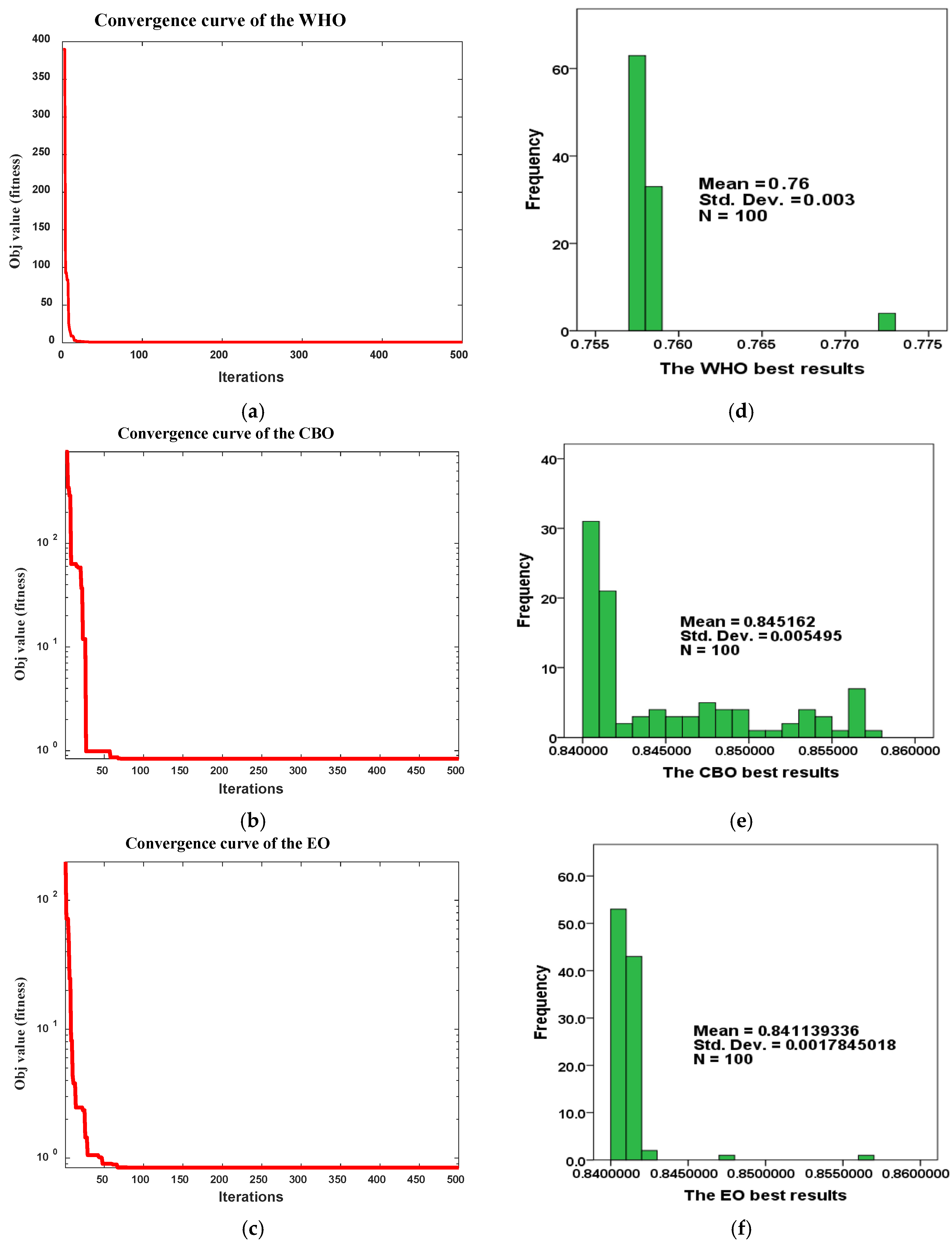
Best fitness (min. Obj)	1.7193	1.1531	1.1659	1.1655	1.3483	1.0897	0.8404196	0.84042	0.7579489
Stand. Deviation	0.00509	1.99 × 10−15	0.008722	1.206342	2.9229	133.37	0.0017755	0.005467	0.002747
Average	1.72133	1.1531	1.176198	1.390042	4.8585	87.573	0.8411393	0.845162	0.758657
Median	1.7199	1.1531	1.17455	1.1773	4.1624	33.951	0.8409335	0.841525	0.757951
Worst fitness (max. Obj)	1.7391	1.1531	1.1937	11.7925	18.323	871.03	0.8569407	0.85763	0.772081
Variance	2.6 × 10−5	4.03 × 10−30	7.684 × 10−5	2.253582	8.6297	17,968.8	3.184 × 10−5	3.019 × 10−5	7.62356 × 10−6
Av_time	8.9540	4.14063	2.75704	33.24938	0.7278	5.3231	0.42235	0.387034	0.3759676

. Despite the convergent outcomes of the best candidates (WHO, CBO and EO), there are some points that need to be clarified. The analysis of 100 individual runs for each optimizer was performed using the criteria of standard deviation, median, variance, worst fitness and average elapsed time. These criteria assured the excellence of the three algorithms according to the convergent results. Considering the slight advantage of the WHO algorithm’s results, further evaluation was carried out to make a strong decision about the candidate algorithm.

Another analysis was performed using the Wilcoxon signed ranks test (a non-parametric analysis) for the top results of (WHO, EO, and CBO). The median total runs of the three candidates were compared considering a significant value of 0.05.

Table 6. Statistical Wilcoxon analysis for WHO versus CBO and EO.

Comparison	WHO-CBO	WHO-EO	CBO-EO
p-value	0	0	0
Positive rank	0	0	27
Negative rank	100	100	73
Decision	Reject null hypotheses	Reject null hypotheses	Reject null hypotheses

describes the outcomes of dual comparisons (p-values, positive rank, and negative rank). Taking a closer look at the table, it is clear that there are significant differences between the total run results for each of the comparative techniques.

Another round of investigations was performed, in which the convergence curves of the closest competitors (WHO, CBO, and EO) were to plotted check their performance, as depicted in Figure 6a–c, respectively. According to Figure 6a, it is clear that the WHO algorithm performed better than CBO and EO in terms of quickly providing a solution. This makes the WHO valid for the objective of online adaptive modeling in this work. On the right side of Figure 6, Figure 6d–f depict histograms of the best solutions of the closest competitors (WHO, CBO and EO), respectively. It can be noticed that for the EO, most of the best solutions are distributed between the values of 0.841 and 0.845, but some solutions are far from this range. This point moderately decreased our expectations of the solutions provided by the EO algorithm. In Figure 6e the CBO histogram shows a wider distributed range of results between (0.84 and 0.86). Moving on to Figure 6f, it is remarkable that most of the solutions are concentrated in a very narrow band with the best result of 0.75. Which supports the reliability of the WHO in finding the best solutions.

The novelty of this work lies in the fact that the elapsed computational time represents a crucial factor for the objective of this work. This factor is of great importance for choosing a suitable technique that satisfies the online PEMFC modeling requirements. In this regard, the WHO-based method achieved the best results at the standard minimum computational time of 0.375 s, surpassing the closest competitor by 0.01106 s. In this regard, the proposed method was applied at different values of maximum iterations and population sizes. A further convergence analysis is performed under different initial population sizes (20, 15, 10, 5) and maximum iteration times (500, 400, 300, 200, 100). The resulting convergence curves are depicted on Figure 7a,b. Taking a closer look at Figure 7a, it is clear that the proposed method reached the best solution before the 50th iteration. This supports the method’s high-speed computing capabilities. In Figure 7b the proposed method achieved the best performance with a population of 20. By decreasing the population size, the method convergence speed is slightly decreased, but reached the best solution before the 80th iteration. These observations confirm the reliability of the proposed method to effectively operate with a minimal computational burden.

As shown in the above remarks, the fast and accurate performance of the WHO creates a clear impression of its reliability in adaptive PEMFC modeling and real-time applications. The reliability of the developed model of the 250 W PEMFC under different operating conditions is expressed by the characteristic curves shown in Figure 8. The developed polarization (V-I) curves show an outstanding match with the actual experimental data for the cell.

In the second stage, further verification of the WHO-based method was carried out by modeling three commercial PEMFC devices. The device named Nedstack-PS6—6 kW was utilized to develop an adaptive model that mimics its performance along its lifetime. The fitness value expressed by the SSE and the elapsed computational time are reported in

Table 7. Nedstack-PS6-6kW PEMFC modeling by WHO-based method (second stage).

Method	Fitness (SSE)	Elapsed Time	${\mathsf{\xi }}_1$	${\mathsf{\xi }}_2$	${\mathsf{\xi }}_3$	${\mathsf{\xi }}_4$	$\mathsf{\Psi }$	${\mathit{R}}_{\mathit{c}}$	$\mathit{B}$
WHO	1.4957	0.3321	−0.9348	2.187 × 10−3	4.07 × 10−5	−1.145 × 10−4	10.000	1.0 × 10−4	0.0727
CBO [37]	1.5734	0.35938	−1.0945	2.881 × 10−3	5.66 × 10−5	−1.162 × 10−4	16.287	1.01 × 10−4	0.1148
VSDE [27]	2.08849	Not reported	1.1212	3.348 × 10−3	4.67 × 10−5	9.54 × 10−5	13.000	1 × 10−4	0.0494
SSO [33]	2.18067	Not reported	0.9719	3.348 × 10−3	7.91 × 10−5	9.543 × 10−5	13.000	1 × 10−4	0.0534
GHO [27]	2.18586	Not reported	1.1997	3.55 × 10−3	4.61 × 10−5	9.54 × 10−5	13.009	1.01 × 10−4	0.0579
VSA [27]	2.34260	Not reported	0.8946	3.348 × 10−3	9.75 × 10−5	9.54 × 10−5	13.000	1.03 × 10−4	0.0429

and the corresponding curve is shown in Figure 9. In comparison to the solutions reported in the literature, it was found that the WHO-based method surpassed the other competitors in terms of accuracy with a minimum SSE of 1.4957 and minimum computational time of 0.3321. From Figure 9, it is clear that the developed model characteristic curve is well matched with experimental data for the real device. Furthermore, the proposed method is designed to deal with the modeling of Nedstack-PS6—6 kW under different operating conditions. The device operating temperature was configured to take the values of 323, 333, 343 and 353 in kelvins (k) and the developed model curves are depicted in Figure 10a. Then, the operating pressures of hydrogen and oxygen were set to values of (${\mathit{P}}_{{\mathit{H}}_2}=0.5 , {\mathit{P}}_{O_2}=0.5$), (${\mathit{P}}_{{\mathit{H}}_2}=1 , {\mathit{P}}_{O_2}=0.5$), (${\mathit{P}}_{{\mathit{H}}_2}=0.25 , {\mathit{P}}_{O_2}=0.5$), (${\mathit{P}}_{{\mathit{H}}_2}=0.5 , {\mathit{P}}_{O_2}=0.25$) and (${\mathit{P}}_{{\mathit{H}}_2}=0.5 , {\mathit{P}}_{O_2}=1$) per atmospheric pressure ($atm$). The resulting curves are shown in Figure 10b. These curves express the reliability of the proposed method in dealing with adaptive modeling tasks under a variety of operating conditions.

In the same context, the WHO-based method is implemented to model a Temasek 1 kW PEMFC in

Table 8. Further investigation of Temasek 1 kW PEMFC model by WHO-based method.

Approach	Fitness	Elapsed Time	${\mathsf{\xi }}_1$	${\mathsf{\xi }}_2$	${\mathsf{\xi }}_3$	${\mathsf{\xi }}_4$	$\mathsf{\Psi }$	${\mathit{R}}_{\mathit{c}}$	$\mathit{B}$
WHO	0.1441	0.28925	−1.1603	3.13 × 10−3	6.03 × 10−5	−9.54 × 10−5	24	1 × 10−4	0.1821
CBO [37]	0.15204	0.29688	−0.94212	2.842 × 10−3	8.70 × 10−5	−9.54 × 10−5	10	0.00059487	0.1319
FPO [27]	0.1881	Not reported	−0.4838	1.0 × 10−3	2.77 × 10−5	−7.578 × 10−5	11.322	1.109 × 10−4	0.1287
GWO [19]	1.6481	Not reported	−1.0299	2.410 × 10−3	4.00 × 10−5	−9.54 × 10−5	10.000	1.087 × 10−4	0.1274

. The experimental data were fed to the method where the outcomes were very promising in terms of accuracy and computational burden in comparison to other techniques. The results are depicted in

Table 9. Further investigation of Ballard-Mark-V 5 kW PEMFC model by WHO-based method.

Approach	Fitness	Elapsed Time	${\mathsf{\xi }}_1$	${\mathsf{\xi }}_2$	${\mathsf{\xi }}_3$	${\mathsf{\xi }}_4$	$\mathsf{\Psi }$	${\mathit{R}}_{\mathit{c}}$	$\mathit{B}$
WHO	0.0006098	0.24	−0.93996	3.022 × 10−3	9.67 × 10−5	−1.195 × 10−4	12.085	0.0008	0.0136
CBO [37]	0.0006159	0.25	−1.1788	0.0028743	3.64 × 10−5	−1.195 × 10−4	12.08	0.0008	0.0136
FPO [14]	0.0006204	Not reported	−1.0257	3.4 × 10−3	6.79 × 10−5	−1.285 × 10−4	15.644	5.29 × 10−4	0.0614
GWO [19]	0.002067	Not reported	−1.1827	3.708 × 10−3	9.36 × 10−5	−1.192 × 10−4	11.76	7.87 × 10−4	0.0136
IFSO [35]	0.784	3.80	−1.12	3.57 × 10−3	8.01 × 10−5	−1.59 × 10−4	22.00	1.00 × 10−4	0.015

besides those of other competing algorithms. The WHO-based method scored 0.1441 at the scale of accuracy with a minimal elapsed time of 0.28 s. The developed model (V-I) characteristics are well-matched to the experimental data points displayed in Figure 11. Additionally, the proposed method was adapted to model Temasek 1 kW under different operating conditions. The device’s operating temperature was configured to the values of 323, 333, 343 and 353 in kelvins (k) and the pressures of hydrogen and oxygen were (${\mathit{P}}_{{\mathit{H}}_2}=0.5, {\mathit{P}}_{O_2}=0.5$), (${\mathit{P}}_{{\mathit{H}}_2}=0.25, {\mathit{P}}_{O_2}=0.5$), (${\mathit{P}}_{{\mathit{H}}_2}=1, {\mathit{P}}_{O_2}=0.5$), (${\mathit{P}}_{{\mathit{H}}_2}=0.5, {\mathit{P}}_{O_2}=0.25$) and (${\mathit{P}}_{{\mathit{H}}_2}=0.5, {\mathit{P}}_{O_2}=1$) per atmospheric pressure ($atm$). From Figure 12a,b, the robustness of the proposed method is clear as it can express the dynamic changes in cell performance according to its varying operating conditions.

The procedure was repeated by applying the WHO-based method to model the commercial device named Ballard-Mark-V—5 kW PEMFC. The solution is listed alongside the comparative methods in Table 9 and the developed characteristic curve is displayed in Figure 13, respectively. The results confirm the accuracy of the WHO-based method by scoring the minimum SSE and minimum consumed time of 0.0006098 and 0.24 s, respectively. The developed characteristic curve depicted in Figure 13 reveals another example of the model’s superiority as it has a perfect match with actual data points for the device. The Ballard Mark-V—5 kW device is supposed to operate under different operating conditions. The modeling process is fed the data for device temperature, using values of 323, 333, 343, and 353 in kelvins (k) and pressures of hydrogen and oxygen as (${\mathit{P}}_{{\mathit{H}}_2}=0.5, {\mathit{P}}_{O_2}=0.5$), (${\mathit{P}}_{{\mathit{H}}_2}=0.25, {\mathit{P}}_{O_2}=0.5$), (${\mathit{P}}_{{\mathit{H}}_2}=1, {\mathit{P}}_{O_2}=0.5$), (${\mathit{P}}_{{\mathit{H}}_2}=0.5, {\mathit{P}}_{O_2}=0.25$) and (${\mathit{P}}_{{\mathit{H}}_2}=0.5, {\mathit{P}}_{O_2}=1$) per atmospheric pressure ($atm$). The resulting model curves are displayed in Figure 14a,b. The figures describe the promising capability of the proposed method in reflecting the cell performance under different operating conditions. The second stage results confirmed the reliability and speed of the proposed WHO-based method, so it is nominated for the online modeling of PEMFCs.

5. Conclusions

In this study, an efficient adaptive modeling criteria is proposed based on the WHO algorithm. The study included the testing and validation of nine recent meta-heuristic optimizers for the online modeling of fuel cells. The accuracy and computational burden represented decisive factors in identifying a suitable technique. The study was designed to be carried out in two stages and deal with four commercial PEMFC devices, namely 250 W PEMFC, Nedstack-PS6 6 kW, Temasek 1 kW and Ballard-Mark-V 5 kW. The results were well matched to the actual data for PEMFCs, and performance speed and corresponding statistical analysis for repetitive results represented the main factors used to determine the best competitor of the WHO algorithm in the first stage. The WHO-based modeling method outperformed the other methods, as it scored 0.7579489 and 0.375 s in terms of accuracy and elapsed time, respectively.

The second stage was used to verify the quality of the proposed WHO-based modeling method in dealing with three commercial PEMFC devices. The solutions assured the reliability of the WHO-based method as it surpassed the comparative techniques. The WHO-based method’s results prove its suitability for real-time applications, as it can reflect dynamical changes in the PEMFC V-I (considering membrane aging) along its lifetime with a minimal computational burden.

References

- Barbir, F. PEM Fuel Cells: Theory and Practice, 2nd ed.; Academic Press: Cambridge, MA, USA, 2012; ISBN 9780123877109. [Google Scholar] [CrossRef]
- Kaur, G. PEM Fuel Cells: Fundamentals, Advanced Technologies, and Practical Application, 1st ed.; Elsevier: Amsterdam, The Netherlands, 2021; ISBN 9780128237083. [Google Scholar] [CrossRef]
- Xing, Y.; Na, J.; Costa-Castell’o, R. Real-time Adaptive Parameter Estimation for a Polymer Electrolyte Membrane Fuel Cell. IEEE Trans Ind. Inform. 2018, 1551, 6048–6057. [Google Scholar] [CrossRef]
- Dimitrova, Z.; Nader, W.B. PEM fuel cell as an auxiliary power unit for range extended hybrid electric vehicles. Energy 2022, 239, 121933. [Google Scholar] [CrossRef]
- Amphlett, J.C.; Baumert, R.M.; Mann, R.F.; Peppley, B.A.; Roberge, P.R.; Harries, T.J. Performance modeling of the Ballard mark-IV solid polymer electrolyte fuel cell. J. Electrochem. Soc. 1995, 142, 9–15. [Google Scholar] [CrossRef]
- Shang, Z.; Hossain, M.M.; Wycisk, R.; Pintauro, P.N. Poly(phenylene sulfonic acid)-expanded polytetrafluoroethylene composite membrane for low relative humidity operation in hydrogen fuel cells. J. Power Sources 2022, 535, 231375. [Google Scholar] [CrossRef]
- Li, Y.; Yang, F.; Chen, D.; Hu, S.; Xu, X. Thermal-physical modeling and parameter identification method for dynamic model with unmeasurable state in 10-kW scale proton exchange membrane fuel cell system. Energy Convers. Manag. 2023, 276, 116580. [Google Scholar] [CrossRef]
- Fletcher, T.; Thring, R.; Watkinson, M. An Energy Management Strategy to concurrently optimise fuel consumption & PEM fuel cell lifetime in a hybrid vehicle. Int. J. Hydrogen Energy 2016, 41, 21503–21515. [Google Scholar] [CrossRef]
- Zhou, D.; Wu, Y.; Gao, F.; Breaz, E.; Ravey, A.; Miraoui, A. Degradation prediction of pem fuel cell stack based on multiphysical aging model with particle filter approach. IEEE Trans. Ind. Appl. 2017, 53, 4041–4052. [Google Scholar] [CrossRef]
- Singh, R.; Sui, P.; Wong, K.; Kjeang, E.; Knights, S.; Djilali, N. Modeling the effect of chemical membrane degradation on pemfc performance. J. Electrochem. Soc. 2018, 165, 3328–3336. [Google Scholar] [CrossRef]
- Xie, R.; Li, C.; Ma, R.; Xu, L.; Zhou, X. An Explainable Data-Driven Framework for Fuel Cell Aging Prediction Under Dynamic Condition. IEEE Trans. Ind. Electron. 2023, 70, 5960–5970. [Google Scholar] [CrossRef]
- Tian, Z.; Wang, J.; Al-Durra, A.; Muyeen, S.; Zhou, D.; Hua, S. A novel aging prediction method of fuel cell based on empirical mode decomposition and complexity threshold quantitative criterion. J. Power Sources 2023, 574, 233120. [Google Scholar] [CrossRef]
- Xing, Y.; Costa-Castelló, R.; Na, J.; Renaudineau, H. Control-oriented modelling and analysis of a solid oxide fuel cell system. Int. J. Hydrogen Energy 2020, 45, 20659–20672. [Google Scholar] [CrossRef]
- Priya, K.; Rajasekar, N. Application of flower pollination algorithm for enhanced proton exchange membrane fuel cell modelling. Int. J. Hydrogen Energy 2019, 44, 18438–18449. [Google Scholar] [CrossRef]
- Seleem, S.I.; Hasanien, H.M.; El-Fergany, A.A. Equilibrium optimizer for parameter extraction of a fuel cell dynamic model. Renew. Energy 2021, 169, 117–128. [Google Scholar] [CrossRef]
- Turgut, O.E.; Coban, M.T. Optimal proton exchange membrane fuel cell modelling based on hybrid Teaching Learning Based Optimization-Differential Evolution algorithm. Ain Shams Eng. J. 2016, 7, 347–360. [Google Scholar] [CrossRef]
- Jia, J.; Li, Q.; Wang, Y.; Cham, Y.; Han, M. Modeling and dynamic characteristic simulation of a Proton Exchange Membrane Fuel Cell. IEEE Trans. Energy Convers. 2009, 24, 283–291. [Google Scholar] [CrossRef]
- Askarzadeh, A.; Rezazadeh, A. A new heuristic optimization algorithm for modeling of proton exchange membrane fuel cell: Bird mating optimizer. Int. J. Energy Res. 2013, 37, 1196–1204. [Google Scholar] [CrossRef]
- Ali, M.; El-Hameed, M.A.; Farahat, M.A. Effective parameters’ identification for polymer electrolyte membrane fuel cell models using grey wolf optimizer. Renew. Energy 2017, 111, 455–462. [Google Scholar] [CrossRef]
- Mo, Z.; Zhu, X.; Wei, L.; Cao, G. Parameter optimization for a PEMFC model with a hybrid genetic algorithm. Int. J. Energy Res. 2006, 30, 585–597. [Google Scholar] [CrossRef]
- Ohenoja, M.; Leiviska, K. Validation of genetic algorithm results in a fuel cell model. Int. J. Hydrogen Energy 2010, 35, 12618–12625. [Google Scholar] [CrossRef]
- Zhu, Q.; Wang, N.; Zhang, L. Circular genetic operators based RNA genetic algorithm for modeling proton exchange membrane fuel cells. Int. J. Hydrogen Energy 2014, 39, 17779–17790. [Google Scholar] [CrossRef]
- Zhang, L.; Wang, N. An adaptive RNA genetic algorithm for modeling of proton exchange membrane fuel cells. Int. J. Hydrogen Energy 2013, 38, 219–228. [Google Scholar] [CrossRef]
- Ye, M.; Wang, X.; Xu, Y. Parameter identification for proton exchange membrane fuel cell model using particle swarm optimization. Int. J. Hydrogen Energy 2009, 34, 981–989. [Google Scholar] [CrossRef]
- Chakraborty, U.K.; Abbott, T.E.; Das, S.K. PEM fuel cell modeling using differential evolution. Energy 2012, 40, 387–399. [Google Scholar] [CrossRef]
- Gong, W.; Yan, X.; Liu, X.; Cai, Z. Parameter extraction of different fuel cell models with transferred adaptive differential evolution. Energy 2015, 86, 139–151. [Google Scholar] [CrossRef]
- Fathy, A.; Abd Elaziz, M.; Alharbi, A. A novel approach based on hybrid vortex search algorithm and differential evolution for identifying the optimal parameters of PEM fuel cell. Renew. Energy 2020, 146, 1833–1845. [Google Scholar] [CrossRef]
- Askarzadeh, A.; Rezazadeh, A. A grouping-based global harmony search algorithm for modeling of proton exchange membrane fuel cell. Int. J. Hydrogen Energy 2011, 36, 5047–5053. [Google Scholar] [CrossRef]
- Yang, S.; Wang, N. A novel P system based optimization algorithm for parameter estimation of proton exchange membrane fuel cell model. Int. J. Hydrogen Energy 2012, 37, 8465–8476. [Google Scholar] [CrossRef]
- Rao, R.; Patel, V. Comparative performance of an elitist teaching-learning-based optimization algorithm for solving unconstrained optimization problems. Int. J. Ind. Eng. Comput. 2013, 4, 29–50. [Google Scholar] [CrossRef]
- Niu, Q.; Zhang, H.; Li, K. An improved TLBO with elite strategy for parameters identification of PEM fuel cell and solar cell models. Int. J. Hydrogen Energy 2014, 39, 3837–3854. [Google Scholar] [CrossRef]
- Guarnieri, M.; Negro, E.; Noto, V.; Alotto, P. A selective hybrid stochastic strategy for fuel-cell multi-parameter identification. J. Power Sources 2016, 332, 249–264. [Google Scholar] [CrossRef]
- El-Fergany, A.A. Extracting optimal parameters of PEM fuel cells using Salp Swarm Optimizer. Renew. Energy 2018, 119, 641–648. [Google Scholar] [CrossRef]
- Rao, Y.; Shao, Z.; Ahangarnejad, A.H.; Gholamalizadeh, E.; Sobhanid, B. Shark Smell Optimizer applied to identify the optimal parameters of the proton exchange membrane fuel cell model. Energy Convers. Manag. 2019, 182, 1–8. [Google Scholar] [CrossRef]
- Qin, F.; Liu, P.; Niu, H.; Song, H.; Yousefi, N. Parameter estimation of PEMFC based on Improved Fluid Search Optimization Algorithm. Energy Rep. 2020, 6, 1224–1232. [Google Scholar] [CrossRef]
- Yakout, A.; Hasanien, H.; Kotb, H. Proton Exchange Membrane Fuel Cell Steady State Modeling Using Marine Predator Algorithm Optimizer. Ain Shams Eng. J. 2021, 12, 3765–3774. [Google Scholar] [CrossRef]
- Ali, M.; Mandour, M.; Lotfy, M. Adaptive Estimation of Quasi-Empirical Proton Exchange Membrane Fuel Cell Models Based on Coot Bird Optimizer and Data Accumulation. Sustainability 2023, 15, 9017. [Google Scholar] [CrossRef]
- Wolpert, D.; Macready, W. No free lunch theorems for optimization. IEEE Trans. Evol. Comput. 1997, 1, 67–82. [Google Scholar] [CrossRef]
- Naruei, I.; Keynia, F. Wild horse optimizer: A new meta-heuristic algorithm for solving engineering optimization problems. Eng. Comput. 2022, 38 (Suppl.4), 3025–3056. [Google Scholar] [CrossRef]
- Ali, M.; Kamel, S.; Hassan, M.; Tostado-Véliz, M.; Zawbaa, H. An improved wild horse optimization algorithm for reliability based optimal DG planning of radial distribution networks. Energy Rep. 2022, 8, 582–604. [Google Scholar] [CrossRef]
- Zhao, W.; Liu, Y.; Li, J.; Zhu, T.; Zhao, K. A Wild Horse Optimization algorithm with chaotic inertia weights and its application in linear antenna array synthesis. PLoS ONE 2024, 19, e0304971. [Google Scholar] [CrossRef]
- Nadimi-Shahraki, M.; Taghian, S.; Mirjalili, S.; Faris, H. MTDE: An effective multi-trial vector-based differential evolution algorithm and its applications for engineering design problems. Appl. Soft Comput. 2020, 97, 106761. [Google Scholar] [CrossRef]
- Zhao, W.; Wang, L.; Zhang, Z. Atom search optimization and its application to solve a hydrogeologic parameter estimation problem. Knowl. Based Syst. 2019, 163, 283–304. [Google Scholar] [CrossRef]
- Mirjalili, S. Dragonfly algorithm: A new meta-heuristic optimization technique for solving single-objective, discrete, and multi-objective problems. Neural Comput. Appl. 2015, 27, 1053–1073. [Google Scholar] [CrossRef]
- Saremi, S.; Mirjalili, S.; Lewis, A. Grasshopper Optimisation Algorithm: Theory and application. Adv. Eng. Softw. 2017, 105, 30–47. [Google Scholar] [CrossRef]
- Faramarzi, A.; Heidarinejad, M.; Stephens, B. Equilibrium optimizer: A novel optimization algorithm. Knowl. Based Syst. 2019, 191, 105190. [Google Scholar] [CrossRef]
- Mirjalili, S. The ant lion optimizer. Adv. Eng. Softw. 2015, 83, 80–98. [Google Scholar] [CrossRef]
- Matlab (R2020a) Is a Product of the MathWorks. Available online: http://www.mathworks.com (accessed on 10 August 2024).
- IBM SPSS (Version 22) Is a Product of the IBM Corporation. Available online: http://www.ibm.com/analytics/us/en/technology/spss/ (accessed on 2 September 2024).