Prediction of Carbon Emissions from Coal-Fired Power Plants During Load Cycling with Varying Coal Characteristics

Abstract

With the evolvement of the coal marketplace and massive growth in renewable resource power, conventional coal-fired generation is facing challenges in the operation of fluctuating loads and varying coal characteristics. The intent of this study is to predict carbon emissions from coal-fired power plants during load cycling and the operation of varying coal characteristics. The given correlation was revised by adding a new nitrogen term and using thermodynamic data from the latest JANAF tables. On the basis of the revised correlation, the quantitative impact of each element composition of coal on the carbon emission factor was worked out according to first-order Taylor series approximation. The O/C and H/C ratio of coal at the lowest carbon emission factor was evaluated in the VAN Krevelen diagram, showing that coals have the lowest carbon emission factor value of roughly 23.25 kg/GJ GCV at atomic O/C and H/C ratio values of about 0.08 and 0.98, respectively. Correlations of carbon emission with the proximate analysis of coal were established through stepwise linear regression using 247 coals for power generation. Based on the varying nature of the net heat rate with load condition expressed by the generic model derived from 11 typical units in-service, the impact of coal and load cycling on carbon emission was captured with a developed equation. Linking the above investigation to a study in a thermal power unit with a rated output of 1000 MW shows that the total variation of carbon emission due to the combined effect of coal and load cycling could be 27.44% if the unit cycles at 35% to 100% rated output with coal normally varying in the present context.

1. Introduction

Carbon dioxide is a potential global warming driver, with a concern in science and politics increasingly focused on. Coal-fired power generation accounts for the largest source of anthropogenic carbon dioxide emissions due to the affordability and abundance of coal as a fuel. As a strategy to reduce carbon emissions, renewable energy has been facilitated to be of massive growth in the past decade [1]. For instance, by the end of 2022, the total installed capacity of renewable resource power in China exceeded 1200 GW, with a 12.2% wind and photovoltaic power supply in aggregated electricity consumption [2]. Integrating intermittent renewable energy into the power system requires balancing services such as cyclic operation from the dispatchable coal-fired generation [3,4]. However, balance service impacts the performance of the conventional power unit by inducing plant efficiency penalty [5,6], and hence, carbon emissions increase due to greater coal volumes consumed [7].

In addition to correlating with cyclic operation, carbon emissions, on the other hand, are significantly dependent on coal characteristics. In order to reduce the cost of generation or increase the use of low-grade coal, it is becoming increasingly common that nationally, at least 70% of power plants, probably significantly more, cannot achieve burning coal with consistent characteristics. As the available coal becomes lower in quality or more expensive, the unprecedentedly broad ranks of coals are utilized in thermal power units originally designed to burn coal with defined characteristics. This could result in a variation in carbon emission due to varying coal characteristics.

Variation of carbon emissions with coal rank is extensively recognized in national greenhouse gas inventories and taken into account using a rank-dependent carbon emission factor, which ranges from 25.8 kg/GJ for bituminous coal to 27.6 kg/GJ for lignite according to the Intergovernmental Panel on Climate Change (IPCC) [8]. Those instructive data from IPCC are mainly based on a large database of coal sample analysis to calculate the average emission factor for each rank category of coal [9] and applicable to compile carbon emission inventories on a macroscopic accounting, for instance, on a national or sector basis [10,11,12,13]. However, this method is subject to significant estimation errors in calculating carbon emissions for a specific power plant [14,15,16]. Carbon emissions increasing from liptinite through vitrinite to inertinite were identified by Sakulpitakphon and Hower for several sets of density-gradient centrifugation maceral concentrates from the highly volatile bituminous coals, which evidenced that there exists a potential misleading on carbon emission estimates if a single value of emission factor is used covering a broad range of coals within a given rank [17]. Quantifying the effect of the individual composition of coal on carbon emission is of special interest because it assists in performing a more accurate estimate of additional carbon emissions incurred by a special component of coal. Winschel calculated carbon dioxide emissions for 504 North American coals to explore the effects of sulfur content on carbon dioxide emissions [18]. Quick and Brill further demonstrated the contribution of either decreasing sulfur content or increasing inertinite content to elevate carbon dioxide emissions from bituminous coal [19]. Another approach to get a better accuracy of prediction is to estimate carbon emissions based on readily available coal analysis measurements rather than on just coal rank. Roy et al. estimated carbon dioxide emissions from basic coal parameters such as VM, FC, and GCV using linear predictive equations, showing that these equations may be utilized to get a realistic estimate of carbon dioxide emissions in specific cases where Indian coals are mostly used [20]. From continuous emissions monitoring data, Dios et al. obtained specific emissions factors for a large 1400 MW coal-fired power plant in various combustion conditions when burning a mixture of lignite and subbituminous coal [21].

Load conditions in thermal generating units are the major factor affecting carbon emissions in the power generation process [22]. A few studies on the effect of load cycling on carbon emission are available in the literature so far. Dong et al. evaluated the environmental impacts of flexible operation using a high-resolution operation dataset from coal-fired power plants [23]; conclusions are drawn based on two case units with capacities of 300 MW and 600 MW, respectively. Akpan and Fuls focused on a generic model for predicting carbon dioxide emissions in the cycling of coal-fired power plants; however, they gave only ’good coal’ and ’bad coal’ to demonstrate the impact of fuel characteristics on carbon emissions [24].

Although a continuous emission monitoring system could be used for carbon emission measurement [25], it is costly, unavailable for some thermal generating units, and either difficult or has large measurement errors in flue gas flow determination [14]. This study attempted to investigate the combined impact of firing coal and cyclic operation on carbon emissions from coal-fired power plants. The carbon emission model presented requires only net thermal efficiency at full load and proximate analysis of coal to estimate carbon emissions. It is of significance in establishing strategies for carbon emission reduction, optimizing balancing service from coal-fired thermal units, and evaluating carbon mitigation benefits in employing renewable energy in the power system. For the sake of convenience, we summarize the key models with calculating examples in

Table 1. The key models with calculating examples.

Equation No	Formula	Data Sample	Results
Equation (16)	$\begin{array}{l}\mathrm{E}\mathrm{F}\left(\mathrm{k}\mathrm{g}/\mathrm{G}\mathrm{J}\mathrm{N}\mathrm{C}\mathrm{V}\right)=25.720+0.066\left[\mathrm{C}\right]-1.456\left[\mathrm{H}\right]+0.161\left[\mathrm{O}\right]\\ +0.008\left[\mathrm{N}\right]-0.113\left[\mathrm{S}\right]+0.034\left[\mathrm{M}\right]+0.004\left[\mathrm{A}\right]\end{array}$	$\left[\mathrm{C}\right]=$ $57.69,\left[\mathrm{H}\right]$ $=3.54,\left[\mathrm{O}\right]$ $=8.00,\left[\mathrm{N}\right]=$ $0.64,\left[\mathrm{S}\right]$ $=1.05,\left[\mathrm{M}\right]$ $=8.37,\left[\mathrm{A}\right]=$ 20.71	$\mathrm{E}\mathrm{F}$ = 25.92
Equation (20)	$\begin{array}{l}\mathrm{E}\mathrm{F}\left(\mathrm{k}\mathrm{g}/\mathrm{G}\mathrm{J}\mathrm{N}\mathrm{C}\mathrm{V}\right)=25.572+0.285\left[\mathrm{F}\mathrm{C}\right]+0.184\left[\mathrm{V}\mathrm{M}\right]-0.281\left[\mathrm{S}\mathrm{t}\right]\\ -0.740 \mathrm{G}\mathrm{C}\mathrm{V}+0.021\left[\mathrm{M}\right]\end{array}$	$\left[\mathrm{F}\mathrm{C}\right]$ $=37.74,\left[\mathrm{V}\mathrm{M}\right]$ $=26.21,\left[\mathrm{M}\right]$ $=9.40,\left[\mathrm{A}\right]$ $=26.65,\left[\mathrm{S}\mathrm{t}\right]$ $=0.58,\mathrm{G}\mathrm{C}\mathrm{V}$ = 20.83 MJ/kg	$\mathrm{E}\mathrm{F}$ = 25.77
Equation (18)	$\begin{array}{l}\mathrm{E}\mathrm{F}\left(\mathrm{k}\mathrm{g}/\mathrm{k}\mathrm{g}\right)=-0.0193+0.0060\left[\mathrm{F}\mathrm{C}\right]+0.0034\left[\mathrm{V}\mathrm{M}\right]-0.0058\left[\mathrm{S}\mathrm{t}\right]\\ +0.0104 \mathrm{G}\mathrm{C}\mathrm{V}\end{array}$	$\left[\mathrm{F}\mathrm{C}\right]$ $=31.93,\left[\mathrm{V}\mathrm{M}\right]$ $=30.06,\left[\mathrm{M}\right]$ $=10.00,\left[\mathrm{A}\right]$ $=27.47,\left[\mathrm{S}\mathrm{t}\right]$ $=2.06,\mathrm{G}\mathrm{C}\mathrm{V}$ = 20.85 MJ/kg	$\mathrm{E}\mathrm{F}$ = 0.4812
Equation (28)	$\begin{array}{l}{\mathrm{E}\mathrm{F}}_{\mathrm{U}}\left(\mathrm{g}/\mathrm{k}\mathrm{W}\mathrm{h}\right)=0.0293\times \mathrm{E}\mathrm{F}\left(\mathrm{k}\mathrm{g}/\mathrm{G}\mathrm{J}\mathrm{N}\mathrm{C}\mathrm{V}\right)\times {\mathrm{B}}_0\times (0.746\\ \times \mathrm{e}\mathrm{x}\mathrm{p}\left(-4.090\times \mathrm{P}/{\mathrm{P}}_0\right)+0.988)\times \alpha \end{array}$	$\mathrm{E}\mathrm{F}=25.92$ $,{\mathrm{B}}_0$ $=325\mathrm{g}/\mathrm{kWh},\mathrm{P}$ $=270\mathrm{MW},{\mathrm{P}}_0$ $=300\mathrm{MW},\alpha$ = 0.985	${\mathrm{E}\mathrm{F}}_{\mathrm{U}}$ = 244.77
Equation (29)	${\mathrm{E}\mathrm{F}}_{\mathrm{U}}\left(\mathrm{g}/\mathrm{k}\mathrm{W}\mathrm{h}\right)={\displaystyle \frac{3.6\times \alpha \times \mathrm{E}\mathrm{F}\left(\mathrm{k}\mathrm{g}/\mathrm{G}\mathrm{J}\mathrm{N}\mathrm{C}\mathrm{V}\right)}{(-0.546\times \mathrm{e}\mathrm{x}\mathrm{p}\left(-3.532\times \mathrm{P}/{\mathrm{P}}_0\right)+1.016){\times \eta }_0}}$	$\mathrm{E}\mathrm{F}=25.77$ $,\alpha$ $=0.99,{\mathrm{P}}_0$ $=997.38\mathrm{MW},\mathrm{P}=600\mathrm{MW},{\eta }_0$ = 0.43	${\mathrm{E}\mathrm{F}}_{\mathrm{U}}$ = 224.65
Equations (2) and (5)	${\mathrm{E}\mathrm{F}}_{\mathrm{U}}\left(\mathrm{g}/\mathrm{k}\mathrm{W}\mathrm{h}\right)=m\times \mathrm{E}\mathrm{F}\left(\mathrm{k}\mathrm{g}/\mathrm{k}\mathrm{g}\right)\times \alpha /{\mathrm{P}}_{\mathrm{N}}$	$\mathrm{E}\mathrm{F}$ $=0.4812,\alpha$ $=0.99,{\mathrm{P}}_{\mathrm{N}}$ $=866.6\mathrm{MW},m$ = 394, 795.9 kg/h	${\mathrm{E}\mathrm{F}}_{\mathrm{U}}$ = 217.03

.

The rest of the paper is organized as follows: in Section 2, we briefly describe the methodology, data collection, net heat rate calculation, and auxiliary power measurement in thermal units. In Section 3, the revised Given correlation is derived to estimate the calorific value of coal, and on the basis of this, we give a comprehensive investigation of the carbon emission factor and elemental composition of coal. We explore the impact of load level on the net heat rate of thermal units in Section 4. Based on the above research, an expression to capture the combined effects of coal and load level on carbon emission is developed in Section 5. These are brought in Section 6, which illustrates the case study in a thermal unit. Finally, we draw conclusions in Section 7.

2. Methodology

2.1. Emission Calculation

The most common expression for estimating carbon emission is set up by combining activity data (AD) with emission factors (EF) as [26]:

$$\mathrm{E}=\mathrm{A}\mathrm{D}\times \mathrm{E}\mathrm{F}$$

(1)

Coal consumption in terms of mass or energy would constitute activity data, and the mass of carbon emitted per unit of fuel consumed would be an emission factor expressed correspondingly as:

$$\mathrm{E}\mathrm{F} (\mathrm{k}\mathrm{g} \mathrm{o}\mathrm{f} \mathrm{c}\mathrm{a}\mathrm{r}\mathrm{b}\mathrm{o}\mathrm{n}/\mathrm{k}\mathrm{g} \mathrm{o}\mathrm{f} \mathrm{c}\mathrm{o}\mathrm{a}\mathrm{l})=\left[\mathrm{C}\right]/100$$

(2)

$$\mathrm{E}\mathrm{F} (\mathrm{k}\mathrm{g} \mathrm{o}\mathrm{f} \mathrm{c}\mathrm{a}\mathrm{r}\mathrm{b}\mathrm{o}\mathrm{n}/\mathrm{G}\mathrm{J})=10\times \left[\mathrm{C}\right]/\mathrm{C}\mathrm{V}$$

(3)

Here, [C] is the carbon percent present in coal as received (ar) basis; CV is the net or gross calorific value (NCV or GCV) with units of GJ/t, and EF is the NCV-based or GCV-based emission factor, correspondingly.

Net power generation (${\mathrm{G}}_{\mathrm{N}}$) is sometimes treated as activity data due to accurate measurements or readily available statistical information; in this case, the emission factor of generation (${\mathrm{E}\mathrm{F}}_{\mathrm{U}}$) is defined as:

$${\mathrm{E}\mathrm{F}}_{\mathrm{U}}=\mathrm{E}/{\mathrm{G}}_{\mathrm{N}}$$

(4)

where ${\mathrm{G}}_{\mathrm{N}}$ is the aggregate net generation with units of MWh, obtained by deducting auxiliary power consumption from gross power generated.

Equation (1) is normally used to prepare the GHG inventory according to national or provincial aggregate data on a macroscopic accounting basis. For a specific coal-fired thermal unit, the coal flow rate can be employed as a substitute for aggregate coal consumption to estimate the carbon emission flow rate. Introducing the coal oxidation rate (α) to correct carbon emission in Equation (1), substituting it into Equation (4), and combing Equations (2) and (3), the carbon emission factor of generation can be expressed as:

$${\mathrm{E}\mathrm{F}}_{\mathrm{U}}=m\times \left[\mathrm{C}\right]\times \alpha /\left({100\times \mathrm{P}}_{\mathrm{N}}\right)$$

(5)

$${\mathrm{E}\mathrm{F}}_{\mathrm{U}}=m\times \mathrm{C}\mathrm{V}\times \mathrm{E}\mathrm{F}\times \alpha /{\mathrm{P}}_{\mathrm{N}}$$

(6)

Here, $m$ (kg/h) is the feeding coal flow rate, ${\mathrm{P}}_{\mathrm{N}}$ (MW) is net power output calculated from:

$${\mathrm{P}}_{\mathrm{N}}={\mathrm{P}}_{\mathrm{G}}-{\mathrm{P}}_{\mathrm{A}}$$

(7)

where ${\mathrm{P}}_{\mathrm{G}}$ is the gross power generated and ${\mathrm{P}}_{\mathrm{A}}$ is the auxiliary power consumption.

The result of dividing $m\times \mathrm{C}\mathrm{V}/{\mathrm{P}}_{\mathrm{N}}$ in Equation (6) by 3600 is the reciprocal of the net thermal efficiency of the electricity generation from coal; thus, Equation (6) becomes:

$${\mathrm{E}\mathrm{F}}_{\mathrm{U}}=3600\times \mathrm{E}\mathrm{F}\times \alpha /\eta$$

(8)

where net thermal efficiency ($\eta$) is expressed as a decimal fraction:

$$\eta ={\mathrm{P}}_{\mathrm{N}}/\left(3600\times m\times \mathrm{C}\mathrm{V}\right)$$

(9)

In China, the net heat rate is normally represented by coal consumption rate for net power production, $\mathrm{B}$, expressed as grams of standard coal equivalent per kWh of electricity production (g sce/kWh). By substituting net thermal efficiency with coal consumption rate, Equation (8) becomes:

$${\mathrm{E}\mathrm{F}}_{\mathrm{U}}=\mathrm{B}\times \mathrm{N}{\mathrm{C}\mathrm{V}}_0\times \mathrm{E}\mathrm{F}\times \alpha$$

(10)

where $\mathrm{N}{\mathrm{C}\mathrm{V}}_0$ is the net calorific value of standard coal, $\mathrm{N}{\mathrm{C}\mathrm{V}}_0$ = 29.271 MJ/kg.

Equations (8) and (10) show that ${\mathrm{E}\mathrm{F}}_{\mathrm{U}}$ is correlated with the net thermal efficiency (or unit net heat rate) and carbon emission factor of coal. The effect of elemental composition on the carbon emission factor of coal, of load level on unit net thermal efficiency, and the combined effect of firing coal and cycling load on ${-\mathrm{E}\mathrm{F}}_{\mathrm{U}}$ are separately discussed in the following sections.

2.2. Coals for Power Generation

A dataset of 247 Chinese coals (See Supplementary Materials for details), ranging in rank from lignite to anthracite, was gathered from coal-fired power plants to explore the impact of coal composition on the carbon emission factor. Coal ranks were assigned on the basis of volatile matter on a dry, ash-free (daf) basis according to scientific classification in China. The analytical data include ultimate analysis, proximate analysis, and gross calorific value, all reported on a received (ar) basis and verified with the Mott-Spooner difference of less than 700 kJ/kg [19]. The reported data comprised the design and verification of coals for boilers as well as coals from field sampling during formal acceptance tests of the thermal units, with the analysis performed between 1994 and 2020. In most cases, proximate and ultimate analyses were performed with a U-THERM muffle furnace, CHN-1000 elemental analyzer, and 5E-S3100 coulomb sulfur analyzer. Gross calorific values were determined with an SDACM-2000 automatic calorimeter.

The range of the dataset for volatile matter, fixed carbon, moisture, ash, carbon, hydrogen, oxygen, nitrogen, and sulfur contents are 4.9% to 33.2%, 29.3% to 71.4%, 2.1% to 24.8%, 3.5% to 44.1%, 39.3% to 71.3%, 1.5% to 4.5%, 0.9% to 12.3%, 0.4% to 2.4%, 0.1% to 4.0%, respectively. Gross calorific values range from 15.72 MJ/kg to 28.86 MJ/kg. Those values varied significantly, covering all types of coal for power generation. Figure 1 shows the whole set of the seven ultimate analysis data (i.e., $\left[\mathrm{C}\right]$, $\left[\mathrm{H}\right]$, $\left[\mathrm{O}\right]$, $\left[\mathrm{N}\right]$, $\left[\mathrm{S}\right]$, $\left[\mathrm{A}\right]$, and $\left[\mathrm{M}\right]$) arranged in stacked area by coal rank. It indicates that the oxygen contents progressively decrease from lignite to anthracite, and the moisture content in anthracite and meager coal is more stable than that in lignite and bituminous coal.

2.3. Thermal Units and Efficiency Performance

A number of thermal units were considered in this paper to investigate net heat rates and auxiliary power fractions at various load conditions. These thermal units span wide categories in terms of capacity, parameters, reheat stages, coal rank, boiler, and pulverizing system configuration, representing the typical coal-fired thermal units currently in operation in China. Information on these units is shown in

Table 2. Range of units investigated.

Designation	Unit Size [MW]	Main Steam Parameters [P/T]	Reheat Stages	Coal Rank	Cooling Technology	Boiler Circulation	Mill Type
A	300	16.7 MPa/540 °C	Single reheat	Bituminous	Wet cooled	Drum	TUBE
B	300	16.7 MPa/540 °C	Single reheat	Anthracite	Wet cooled	Drum	TUBE
C	350	24.2 MPa/566 °C	Single reheat	Bituminous	Wet cooled	Once through	ZGM
D	600	17.1 MPa/540 °C	Single reheat	Bituminous	Wet cooled	Drum	TUBE
E	600	17.31 MPa/541 °C	Single reheat	Bituminous	Dry cooled	Drum	MPS
F	600	24.2 MPa/566 °C	Single reheat	Bituminous	Wet cooled	Once through	MPS
G	660	25.1 MPa/571 °C	Single reheat	Meagre	Wet cooled	Once through	TUBE
H	670	24.2 MPa/566 °C	Single reheat	Bituminous	Wet cooled	Once through	HP
I	670	24.2 MPa/566 °C	Single reheat	Bituminous	Wet cooled	Once through	HP
J	1000	26 MPa/605 °C	Single reheat	Bituminous	Wet cooled	Once through	TUBE
K	1000	31 MPa/600 °C	Double reheat	Bituminous	Wet cooled	Once through	MPS

.

The consumption rate of hypothetical coal with NCV of 29,271 kJ/kg, expressed in g sce/kWh of net electricity supplied to the grid, is commonly used as a proxy for the net heat rate of generation. This means if the standard coal consumption rate is 300 g sce/kWh, the net heat rate of the unit is 300/1000 × 29,271 = 8781 kJ/kWh. These two designations of ‘coal consumption rate’ and ‘net heat rate’ are used interchangeably in this paper. The standard coal consumption rate is calculated as [27]:

$$\mathrm{B}={\displaystyle \frac{\mathrm{H}}{29.308\left({\eta }_{\mathrm{b}}/100\right)\left(1-\xi /100\right)\left({\eta }_{\mathrm{p}}/100\right)}}$$

(11)

Here, $\mathrm{H}$ is turbo-generator heat rate (kJ/kWh); ${\eta }_{\mathrm{b}}$ is boiler efficiency on an NCV percent basis (%); $\xi$ is the auxiliary power fraction of the unit (%); and ${\eta }_{\mathrm{p}}$ is pipe efficiency usually set at 99.5%.

Data on boiler efficiency and turbo-generator heat rate at various load levels in normal operation are taken from the performance calculation sheet provided by the manufacturers. Auxiliary power fractions are calculated using an empirical equation.

2.3.1. Boiler Efficiency

Boiler efficiencies at different load conditions were collected from eight steam boilers of various types, referring to units B, C, D, E, F, G, J, and K in Table 2. As indicated in Figure 2a, boiler efficiencies might either increase or decrease as the gross load decreases, reaching as high as 95.08% and as low as 90.4%. However, there is only a slight variation in efficiencies for the same boiler as the load varies. The smallest variation is 0.52% for the boiler of unit G, as the load varies from 30% to 112% rated output, while the largest is 1.72% for unit B. The largest variation in boiler efficiencies for unit B is due to significantly increased combustion losses at lower load conditions because the fired anthracite coal is difficult to burn out when combustion temperature decreases.

2.3.2. Turbo-Generator Heat Rate

The turbo-generator heat rate is plotted as a function of gross load in Figure 2b, indicating that the heat rate is more regular than that of boiler efficiency. Heat rate decreases with a rise in load, which is a similar trend for all thermal units. Variation of the turbo-generator heat rate is more remarkable than that of boiler efficiency when the gross load varies from 30% to 100% rated output. The turbo-generator heat rate decreases by an average of 13% in the mentioned load range (except unit I), while the boiler efficiency only changes by an average of 1%, which means the turbo-generator has a greater impact on the coal consumption rate (Equation (11)) than the boiler as the unit load varies.

2.3.3. Auxiliary Power Measurement

The auxiliary power is used to drive all the auxiliary equipment like mills, fans, pumps, dust removal, desulfurization systems, etc. The auxiliary power fraction is defined as auxiliary power consumption in the percentage of gross power generation:

$$\xi ={\mathrm{P}}_{\mathrm{A}}/{\mathrm{P}}_{\mathrm{G}}\times 100$$

(12)

where ${\mathrm{P}}_{\mathrm{A}}$ is the auxiliary power consumed and ${\mathrm{P}}_{\mathrm{G}}$ is the gross power generated by the unit.

Auxiliary power measurements were achieved in the commissioning and performance assessment tests of those newly installed units (units A, E, K, J, I, and H in Table 2) at that time. The auxiliary power consumed was measured at the High-Voltage Unit Auxiliary Transformer (HUAT) bus using conventional instruments that were equipped for normal monitoring of the units. Sometimes, supplementary measurement for power consumed by a flue gas desulfurization system is desirable when a separate transformer is equipped for this system. In most cases, auxiliary power consumption also includes the power output from the common station service transformer, which is used to run the common auxiliaries for the total station (more than one unit). In this situation, the common auxiliary power divided is proportional to the power generation of the unit.

Auxiliary power consumptions were measured at various load conditions of the units. Based on that measurement, an empirical correlation is established to estimate auxiliary power fraction at various loads (Section 4.1).

3. Effect of Coal on Carbon Emissions

The carbon emission factor of coal, EF, reflects the ratio of carbon to heat content, and thus, the correlations of calorific value expressed in elemental compositions provide practical instruction in investigating the effects of elemental composition on the carbon emission factor. In the published literature, the gross calorific value is calculated from ultimate analysis normally on a dry (d) or a dry and ash-free (daf) basis as:

$$\mathrm{G}\mathrm{C}\mathrm{V}=a_0+a_1\left[\mathrm{C}\right]+a_2\left[\mathrm{H}\right]+a_3\left[\mathrm{O}\right]+a_4\left[\mathrm{N}\right]+a_5\left[\mathrm{S}\right]+a_6\left[\mathrm{A}\right]$$

(13)

In the formula above, $\left[\mathrm{C}\right]$, $\left[\mathrm{H}\right]$, $\left[\mathrm{O}\right]$, $\left[\mathrm{N}\right]$, $\left[\mathrm{S}\right]$, and $\left[\mathrm{A}\right]$ are the contents of carbon, hydrogen, oxygen, nitrogen, sulfur, and ash in weight percentage, respectively. The values of coefficients $a_i$ (i = 0, 1, 2, …, 6) for such eight correlations are given in

Table 3. Literature correlations and estimation errors.

Equation	Investigator	Basis	a0	a1	a2	a3	a4	a5	a6	AAE 1	RMSE 1	MEAN 1	SD 1
Equation (1)	Dulong (1820) [28]	daf		0.3383	1.4430	−0.1804		0.0942		1.49	0.41	0.13	0.39
Equation (2)	Mendeleev (1897) [29]	d		0.3391	1.2560	−0.1090		0.1090		1.29	0.36	−0.01	0.36
Equation (3)	Mott Spooner (1940) [30]	daf		0.3361	1.4190	f 2		0.0942		1.42	0.39	0.11	0.37
Equation (4)	Boie (1952) [31]	daf		0.3517	1.1625	−0.1110	0.0628	0.1047		2.25	0.60	0.46	0.37
Equation (5)	IGT (1978) [32]	d		0.3410	1.3230	−0.1199	−0.1199	0.0684	−0.0153	1.74	0.49	−0.26	0.41
Equation (5)	Given (1985) [33]	daf	0.2730	0.3278	1.4190	−0.1380		0.0926		1.35	0.38	−0.09	0.37
Equation (6)	Neavel et al. (1985) [34]	d		0.3394	1.3249	−0.1254		0.1002	−0.0147	1.59	0.45	−0.22	0.39
Equation (7)	Channiwala (2002) [35]	d		0.3491	1.1783	−0.1034	−0.0151	0.1005	−0.0211	1.65	0.46	−0.17	0.43
Equation (8)	PS 3	daf	0.3469	0.3276	1.4179	−0.1324	−0.0064	0.0926		1.33	0.38	−0.08	0.38

¹ $\mathrm{A}\mathrm{A}\mathrm{E}\left(\%\right)=\sum (\left|e_i\right|/M_i)\times 100/n$; $\mathrm{R}\mathrm{M}\mathrm{S}\mathrm{E}=\sqrt{\sum {e_i}^2/n}$; $\mathrm{M}\mathrm{E}\mathrm{A}\mathrm{N}=\sum e_i/n$; $\mathrm{S}\mathrm{D}=\sqrt{\sum {{(e}_i-\mathrm{M}\mathrm{E}\mathrm{A}\mathrm{N})}^2/\left(n-1\right)}$; $e_i=P_i{-M}_i$; P_i: the predicted value; M_i: the measured value. ² [O] ≤ 15%, f = −0.1454; [O] > 15%, f = −0.1532 − 0.0007211 [O]. ³ Present Study.

, corresponding to the gross calorific value with units of MJ/kg.

Correlations by Mendeleev [29], Boie [31], IGT [32], and Channiwala [35] are purely empirical equations based on large datasets of calorific values and elemental composition of coal. Dulong [28] and Mott Spooner [30] gave similar coefficient values for C, H, and S, respectively. Each value is closely related to the thermodynamically calculated heat of the combustion of the element, and more or less, an empirical correction, especially on the coefficient value for C, is made to offset the effect of the neglected enthalpy of the formation of coal [33]. The enthalpy of formation is defined as the difference between the experimentally determined heating value and the thermodynamically calculated heating value of coal [29]. Given et al. excluded empirical adjustments and used the thermodynamically calculated heating value of the element from JANAF tables as the coefficient of C, H, and S, respectively [33]; for the sake of this, he included an intercept term explicitly related to the enthalpy of formation in his formulae. Although excluding the nitrogen term, the Given model is found to give a more reasonable prediction accuracy in the published literature [33,34,36]. This is because nitrogen content is typically very low in most coals.

3.1. Revised Given Correlation

To investigate the potential impact of nitrogen levels in coal on carbon emissions, we modified the Given correlation by adding a new nitrogen term and using heating values of the combustion of the elements from the latest JANAF tables. The value of the coefficient for the nitrogen term in the new equation is based on combustion products in a coal-fired utility boiler furnace rather than in an adiabatic bomb calorimeter in the laboratory. Combustion products of nitrogen, which dominate the heating value, are diverse and closely related to the air and coal ratio in the primary combustion zone in the furnaces of large utility boilers. Based on nitrogen oxide concentration measurement at the field furnace outlet, it is reasonable to assume that 10% of nitrogen in coal is converted into NO and the rest into N2 in furnace combustion. From this assumption, one can determine the value of the coefficient for the nitrogen term in the present study (PS) in Table 3.

A dataset of 150 coal samples randomly extracted from the total dataset of 247 coals was employed to derive the values of $a_0$ and $a_3$ in Equation (13); a least-squares line is shown in Figure 3. The remaining dataset (97 coals) had been adopted fairly to validate all the selected correlations in Table 3.

The performances of the existing correlations are compared by calculating the residuals of the predicted values. Based on those calculated residuals, Table 3 presents three forms of estimation errors, including the average absolute error (AAE), root mean squared error (RMSE), mean (MEAN), and standard deviation (SD) for the residuals.

Table 3 shows that all the existing models present a good correlation of calorific value; however, correlations by Mendeleev, Given et al., and Mott Spooner give lower estimation errors in terms of either AAE or RMSE and, thereby, a better accuracy of prediction. Of the existing correlations, Dulong, IGT, Neavel, and Channiwala yield intermediate estimation errors, while the Boie correlation, with the largest MEAN value of 0.46, normally suggesting the presence of systematic bias, yields the largest RMSE value of 0.60. This agrees with the results presented earlier [32,34] that the Boie correlation has a large positive MEAN value of the residuals and seriously overestimates the gross calorific value of coal. However, the Boie model might perform well when applied to other fuel types, such as brown coals [37], shale oils [38], and biomass [31]. The estimation error of the revised Given correlation in the present study is comparable to that of the Given correlation.

It is interesting to note that the Mendeleev correlation is superior to all the literature correlations according to AAE and RMSE and remains to be further validated with extensive data of coals.

Using a dataset of coals of various ranks and geological origin from the published literature, the Given model and its revised version were compared with the well-known Mott Spooner correlation, which had received extensive examination and been used to identify gross analytical error in the determination of calorific value or elemental composition of coals [19,39]. The comparative data are presented in

Table 4. GCV estimation errors of the Given model, its revised version, and Mott Spooner correlation.

Ref.	Coal Origin	Number of Coals	Revised/Given Model			Mott Spooner Correlation
			MEAN	SD	RMSE	MEAN	SD	RMSE
[34]	US	66	0.01	0.26	0.26	0.16	0.23	0.28
[33]	US	1004	0	0.55	0.55	0.06	0.54	0.54
[36]	Indian	160	−0.10	0.56	0.57	−0.25	0.62	0.67
PS 1	China	247	0.09	0.37	0.38	0.16	0.36	0.50

¹ PS: Present Study.

. It shows that the Given model and its revised version give a smaller absolute MEAN value and an SD value roughly equivalent to that from the Mott Spooner correlation and combine to provide a smaller RMSE value, showing a slight superiority over the Mott Spooner correlation.

Apart from its accuracy, the revised Given correlation is noteworthy for presenting a heat value for each component of coal individually, which is crucial for analyzing the impact of each elemental composition on the carbon emission factor of coal.

The revised Given correlation was employed to investigate the contribution of each element on calorific value in Section 3.2, to correlate the carbon emission factor with element contents in Section 3.3, and to evaluate the composition of coals having the lowest carbon emission factor in Section 3.4.

3.2. Source of Calorific Value

The revised Given correlation has been reported to predict gross calorific value on a daf basis (Table 3); it might be tuned to predict the net or gross calorific value on an ar basis as:

$$\mathrm{C}\mathrm{V}=b_0+b_1\left[\mathrm{C}\right]+b_2\left[\mathrm{H}\right]+b_3\left[\mathrm{O}\right]+b_4\left[\mathrm{N}\right]+b_5\left[\mathrm{S}\right]+b_6\left[\mathrm{M}\right]+b_7\left[\mathrm{A}\right]$$

(14)

where $\mathrm{C}\mathrm{V}$ is net or gross calorific value. Values for coefficients, b_i (i = 0, 1, …, 7), are included in

Table 5. Coefficients in Equation (14) for predicting calorific value on an as-received basis.

Correlation	b0	b1	b2	b3	b4	b5	b6	b7
GCV	0.3469	0.3276	1.4179	−0.1324	−0.0064	0.0926	−0.0035	−0.0035
NCV	0.3469	0.3276	1.1981	−0.1324	−0.0064	0.0926	−0.0279	−0.0035

.

Heat produced or reduced from each component is definitely represented by the respective term in Equation (14). Negative coefficients for oxygen, nitrogen, moisture, and ash suggest reduced heat by these components; positive coefficients for the remainder terms mean generating heat. The percentage to net calorific value from each component contribution is arranged in a stacked area for 65 data points of representative samples of various coal, as shown in Figure 4. As the major component of coal, carbon is the principal source of heat, with a contribution to a net calorific value ranging from 79% to 92%, with an average of about 87%. Although hydrogen accounts for only 1.5 to 4.5 mass percent of coal, heat generated from hydrogen is second only to carbon, accounting for 8% to 26% and an average of 17% of net calorific value. Oxygen and moisture reduce net calorific value during the combustion of coal, and contribution percentages are accordingly depicted in the negative direction of the ordinate axis. The amount of heat emitted from the combustion of sulfur is relatively small, accounting for an average of only 0.35% of the net calorific value. The absolute net calorific values reduced by nitrogen and ash are, on average, 6 kJ and 81 kJ per unit mass of coal, respectively, accounting for no more than 0.03% and 0.4% of net calorific value; therefore, contributions of the two components are trivial.

3.3. The Derivated Expression of Carbon Emission Factor

The calculation of carbon emissions per unit of calorific value is accomplished with Equation (3), substituting Equation (14) into Equation (3) and solving for $\mathrm{E}\mathrm{F}$:

$$\mathrm{E}\mathrm{F}=10\times {\displaystyle \frac{\left[\mathrm{C}\right]}{b_0+b_1\left[\mathrm{C}\right]+b_2\left[\mathrm{H}\right]+b_3\left[\mathrm{O}\right]+b_4\left[\mathrm{N}\right]+b_5\left[\mathrm{S}\right]+b_6\left[\mathrm{M}\right]+b_7\left[\mathrm{A}\right]}}$$

(15)

Making use of the first order Taylor series approximation of $\mathrm{E}\mathrm{F}$, the carbon emission factor is approximately calculated as follows:

$$\mathrm{E}\mathrm{F}\approx {\mathrm{E}\mathrm{F}}_{\mathrm{B}}+k_{\mathrm{C}}∆\mathrm{C}+k_{\mathrm{H}}∆\mathrm{H}+k_{\mathrm{O}}∆\mathrm{O}+k_{\mathrm{N}}∆\mathrm{N}+k_{\mathrm{S}}∆\mathrm{S}+k_{\mathrm{M}}∆\mathrm{M}+k_{\mathrm{A}}∆\mathrm{A}$$

(16)

Here, ${\mathrm{E}\mathrm{F}}_{\mathrm{B}}$ is the carbon emission factor of the base coal. For the NCV basis, ${\mathrm{E}\mathrm{F}}_{\mathrm{B}}$ = 26.15 kg/GJ; for the GCV basis, ${\mathrm{E}\mathrm{F}}_{\mathrm{B}}$ = 25.09 kg/GJ. The deviations of elemental contents are calculated as: $∆\mathrm{C}=\left[\mathrm{C}\right]-{\left[\mathrm{C}\right]}_{\mathrm{B}}$, $∆\mathrm{H}=\left[\mathrm{H}\right]-{\left[\mathrm{H}\right]}_{\mathrm{B}}$, $∆\mathrm{O}=\left[\mathrm{O}\right]-{\left[\mathrm{O}\right]}_{\mathrm{B}}$, $∆\mathrm{N}=\left[\mathrm{N}\right]-{\left[\mathrm{N}\right]}_{\mathrm{B}}$, $∆\mathrm{S}=\left[\mathrm{S}\right]-{\left[\mathrm{S}\right]}_{\mathrm{B}}$, $∆\mathrm{M}=\left[\mathrm{M}\right]-{\left[\mathrm{M}\right]}_{\mathrm{B}}$, and $∆\mathrm{A}=\left[\mathrm{A}\right]-{\left[\mathrm{A}\right]}_{\mathrm{B}}$. The elemental contents of the base coal are as follows: ${\left[\mathrm{C}\right]}_{\mathrm{B}}=$ 57.19, ${\left[\mathrm{H}\right]}_{\mathrm{B}}=$ 3.12, ${\left[\mathrm{O}\right]}_{\mathrm{B}}=$ 5.63, ${\left[\mathrm{N}\right]}_{\mathrm{B}}=$ 0.93, ${\left[\mathrm{S}\right]}_{\mathrm{B}}=$ 0.96, ${\left[\mathrm{A}\right]}_{\mathrm{B}}=$ 23.22, and ${\left[\mathrm{M}\right]}_{\mathrm{B}}=$ 8.95.

Coefficients of k_C, k_H, k_O, k_N, k_S, k_A, and k_M in Equation (16) are the partial derivatives of $\mathrm{E}\mathrm{F}$ over $\left[\mathrm{C}\right]$, $\left[\mathrm{H}\right]$, $\left[\mathrm{O}\right]$, $\left[\mathrm{N}\right]$, $\left[\mathrm{S}\right]$, $\left[\mathrm{A}\right]$, and $\left[\mathrm{M}\right]$, respectively.

Table 6. Derivative of $\mathrm{E}\mathrm{F}$ over each component and its averaged value on a dataset of coals.

Designation	${\mathit{k}}_{\mathbf{C}}$	${\mathit{k}}_{\mathbf{H}}$	${\mathit{k}}_{\mathbf{O}}$	${\mathit{k}}_{\mathbf{N}}$	${\mathit{k}}_{\mathbf{S}}$	${\mathit{k}}_{\mathbf{M}}$	${\mathit{k}}_{\mathbf{A}}$
Derivative	${\displaystyle \frac{\partial \left(\mathrm{E}\mathrm{F}\right)}{\partial \left(\left[\mathrm{C}\right]\right)}}$	${\displaystyle \frac{\partial \left(\mathrm{E}\mathrm{F}\right)}{\partial \left(\left[\mathrm{H}\right]\right)}}$	${\displaystyle \frac{\partial \left(\mathrm{E}\mathrm{F}\right)}{\partial \left(\left[\mathrm{O}\right]\right)}}$	${\displaystyle \frac{\partial \left(\mathrm{E}\mathrm{F}\right)}{\partial \left(\left[\mathrm{N}\right]\right)}}$	${\displaystyle \frac{\partial \left(\mathrm{E}\mathrm{F}\right)}{\partial \left(\left[\mathrm{S}\right]\right)}}$	${\displaystyle \frac{\partial \left(\mathrm{E}\mathrm{F}\right)}{\partial \left(\left[\mathrm{M}\right]\right)}}$	${\displaystyle \frac{\partial \left(\mathrm{E}\mathrm{F}\right)}{\partial \left(\left[\mathrm{A}\right]\right)}}$
Equation	10${\displaystyle \frac{\mathrm{C}\mathrm{V}-b_1\left[\mathrm{C}\right]}{{\mathrm{C}\mathrm{V}}^2}}$	−10${\displaystyle \frac{b_2\left[\mathrm{C}\right]}{{\mathrm{C}\mathrm{V}}^2}}$	−10${\displaystyle \frac{b_3\left[\mathrm{C}\right]}{{\mathrm{C}\mathrm{V}}^2}}$	−10${\displaystyle \frac{b_4\left[\mathrm{C}\right]}{{\mathrm{C}\mathrm{V}}^2}}$	−10${\displaystyle \frac{b_5\left[\mathrm{C}\right]}{{\mathrm{C}\mathrm{V}}^2}}$	−10${\displaystyle \frac{b_6\left[\mathrm{C}\right]}{{\mathrm{C}\mathrm{V}}^2}}$	−10${\displaystyle \frac{b_7\left[\mathrm{C}\right]}{{\mathrm{C}\mathrm{V}}^2}}$
Averaged derivative of ${\mathrm{E}\mathrm{F}}_{\mathrm{C}}$ (kg/GJ NCV)	0.066	−1.456	0.161	0.008	−0.113	0.034	0.004
Averaged derivative of ${\mathrm{E}\mathrm{F}}_{\mathrm{C}}$ (kg/GJ GCV)	0.079	−1.585	0.148	0.007	−0.104	0.004	0.004

lists formulas to calculate those coefficients. The average values of the coefficients on a total of 247 coals (cf. Table 6) are presented to estimate the carbon emission factor on an NCV or GCV basis.

Equation (16) gives a linear dependence of the carbon emission factor on the elemental compositions of coal. Due to the theoretical considerations on calorific value correlation, coefficients in Equation (16) could be considered as variation rates of carbon emission factor over elemental contents. Thus, one can conclude from Table 6 that carbon emission factors on an NCV basis rise by about 0.066, 0.161, 0.008, 0.034, and 0.004 kg C/GJ for each percentage increment of $[\mathrm{C}$], $[\mathrm{O}$], $[\mathrm{N}$], $[\mathrm{M}$], and $[\mathrm{A}$] in wt.% ar basis, respectively, decline by 1.456 and 0.113 kg C/GJ for each respective percentage increment of $[\mathrm{H}$] and $[\mathrm{S}$] in wt.% ar basis. Carbon emission factors on GCV basis are increased by 0.079, 0.148, 0.007, 0.004, and 0.004 kg C/GJ for each percentage increment of $[\mathrm{C}$], $[\mathrm{O}$], $[\mathrm{N}$], $[\mathrm{M}$], and $[\mathrm{A}$] in wt.% ar basis, respectively, decreases by 1.585 and 0.104 kg C/GJ for each respective percentage increment of $[\mathrm{H}$] and $[\mathrm{S}$] in wt.% ar basis.

Figure 5 shows the deviations of the predicted carbon emission factor values using Equation (16). It can be seen that predicted carbon emission factor data points are close to the straight line, showing a good correlation.

Winschel [17], Quick [18], and Mastalerz [40] explored the effects of elemental contents on the carbon emission factor of coal. The definite conclusions are currently limited to the influence of sulfur elements. Winschel gave a linear regression of CO₂ emissions with sulfur content in the high-volatile bituminous coals, indicating a reduced equivalent carbon emission value of 0.175 kgC/GJ with each percentage increment of $[\mathrm{S}$] in wt.% dry basis. However, the regression coefficient of determination (R²) for his linear model was 0.49, showing that sulfur content accounts for about half the variance in the calculated emissions. By calculating a theoretical, sulfur-free carbon emission factor of 52 Australian and 44 US bituminous coals, Quick showed that the carbon emission factor on NCV basis declined by about 0.08 kgC/GJ for each percentage increment of S in wt.% dry basis, similar to the results presented in this study. Mastalerz believed that an increase in sulfur content results in lower carbon emissions; nevertheless, the impact of $[\mathrm{H}$], $[\mathrm{O}$], $[\mathrm{M}$], and $[\mathrm{A}$] on carbon emissions were considered vague due to the combination of many, often contradicting factors.

3.4. Coals with Lowest Carbon Emission Factor

Searching for coal with minimal carbon emission not only has academic significance but also provides practical assistance for electric utilities in selecting coal for power generation. Equation (3) indicates that for an element other than carbon in coal, the less heat produced by this element during combustion, the smaller its impact on the carbon emission factor. Figure 4 shows that the heat contributions of nitrogen and sulfur to the calorific value are very small, averaging about 0.03% and 0.4%, respectively. The enthalpy of formation (the intercept term) accounts for about 1.74% of the calorific value of coal. Neglecting these three heat sources, the carbon emission factor on a GCV basis is calculated by combining Equation (3) and the revised Given correlation as follows:

$$\mathrm{E}\mathrm{F}={\displaystyle \frac{1}{0.3276+0.1190y-0.1764x}}$$

(17)

where x and y are atomic O/C and H/C ratios of coal, respectively.

The VAN Krevelen plot showing how the atomic H/C ratios vary with the atomic O/C ratios is normally used to display related coal composition. Figure 6 is the VAN Krevelen plot for coals from this study as well as from an extensive literature review by Richards et al. [31]. As can be seen, 94% of the data points are located in the area enclosed by lines of x = 0.015, L_l, x = 0.4, and L_u, which are commonly called coal bands. To locate a position in the above-enclosed area that minimizes EF, the built-in optimizer in Matlab 2018(fmincon) was used to search for the H/C and O/C ratio values meeting the requirement. Column I in

Table 7. The lowest carbon emission factors of a hypothetical organic compound and actual coal.

Parameters	I	II	III
type	ideal	actual	actual
Country		CN	US
Coal Rank		bit	hvBb
$\left[\mathrm{C}\right]$	84.52	79.37	76.05
$\left[\mathrm{H}\right]$	6.91	6.58	5.87
$\left[\mathrm{O}\right]$	8.57	8.34	7.63
$\left[\mathrm{N}\right]$		2.02	1.65
$\left[\mathrm{S}\right]$		3.69	8.70
GCV daf (MJ/kg)	36.35	36.29	33.18
$\mathrm{E}\mathrm{F}$ min (kg/GJ GVC)	23.25	22.73	22.92
x	0.08	0.08	0.08
y	0.98	0.99	0.92

presents optimal results of element content, minimum $\mathrm{E}\mathrm{F},$ and calorific value of the ideal organic compound consisting of only C, H, and O. The pink circle in Figure 6 indicates the location of the minimum EF data point, which is on the ‘shoulder’ of the coal band in the Van Krevelen diagram. The author, thus, concludes that the hypothetical organic compound composed of C, H, and O has the smallest carbon emission factor when the H/C ratio equals 0.08 and the O/C ratio equals 0.98.

Among the 247 coals in this study, the coal with the lowest carbon emission factor is presented in column II of Table 7. Seeking other actual coal with the lowest carbon emission factor in a broader region was conducted by analyzing a dataset of 352 coals around the world. The dataset was generated from the literature review by Richard et al. [31]. The Mott-Spooner test was performed with the dataset to identify whether there are significant analytical errors in calorific value or elemental composition data [19,41]. Any data sample with a Mott-Spooner difference greater than 700 kJ/kg was excluded from further consideration. The coal having the lowest carbon emission factors was listed in column III of Table 7.

Columns II & III in Table 7 show that actual coals have the lowest carbon emission factor value of 22.73 to 22.92 kg C/GJ GCV at atomic O/C and H/C ratios of 0.08 and 0.92–0.99, respectively, which is similar to the calculated results listed in column I in Table 7.

3.5. Stepwise Correlations with Proximate Analysis

Equation (16) is used to estimate the carbon emission of coal from elemental analysis. It is of more practical significance to estimate carbon emissions from what has been referred to as a ‘long proximate analysis’, i.e., gross calorific value (GCV), volatile matter (VM), fixed carbon (FC), moisture content (M), ash yield (A), and total sulfur (St) because this analysis is more readily available than elemental analysis. We introduce stepwise multiple linear regression models to correlate carbon emission factors with the proximate analysis of coal. The candidate variables in the initial stepwise regression model are selected as GCV, VM, FC, M, and St on an ar basis. Ash yield is removed because it can be calculated by difference (i.e., [A] = 100 − [VM] − [FC] − [M]). Stepwise linear regression is recursively constructed by backward elimination that involves dropping candidate variables to remove multicollinearity when they are found to be nonsignificant according to an F-test. Therefore, the stepwise regression is designed to leave a minimum set of independent variables while minimizing the sum of squared error and maximizing the predictive power of the model. The predictive models were obtained by stepwise linear regression using stepwiselm in MATLAB as:

$$\mathrm{E}\mathrm{F}\left(\mathrm{k}\mathrm{g}/\mathrm{k}\mathrm{g}\right)=-0.0193+0.0060\left[\mathrm{F}\mathrm{C}\right]+0.0034\left[\mathrm{V}\mathrm{M}\right]-0.0058\left[\mathrm{S}\mathrm{t}\right]+0.0104 \mathrm{G}\mathrm{C}\mathrm{V}$$

(18)

$$\mathrm{E}\mathrm{F}\left(\mathrm{k}\mathrm{g}/\mathrm{G}\mathrm{J}\mathrm{G}\mathrm{C}\mathrm{V}\right)=24.045+0.274\left[\mathrm{F}\mathrm{C}\right]+0.161\left[\mathrm{V}\mathrm{M}\right]-0.251\left[\mathrm{S}\mathrm{t}\right]-0.672 \mathrm{G}\mathrm{C}\mathrm{V}$$

(19)

$$\mathrm{E}\mathrm{F}\left(\mathrm{k}\mathrm{g}/\mathrm{G}\mathrm{J}\mathrm{N}\mathrm{C}\mathrm{V}\right)=25.572+0.285\left[\mathrm{F}\mathrm{C}\right]+0.184\left[\mathrm{V}\mathrm{M}\right]-0.281\left[\mathrm{S}\mathrm{t}\right]-0.740 \mathrm{G}\mathrm{C}\mathrm{V}+0.021\left[\mathrm{M}\right]$$

(20)

The coefficient of determination (R²) and root mean squared error (RMSE) of the estimate for Equation (18) are 0.99 and 0.008, respectively; for Equation (19), R² = 0.758 and RMSE = 0.380; for Equation (20), R² = 0.764 and RMSE = 0.366.

As can be seen, the correlation for predicting the carbon emission factor on the GCV basis [Equation (19)] is eventually reduced to four explanatory variables, and predicting the carbon emission factor on the NCV basis [Equation (18)] has selected all five candidate variables. The gross calorific value corresponds to the heat produced by combustion where water in the products remains as liquid, being precisely the state it exists in coals originally; accordingly, there is no heat absorbed or emitted in that moisture during combustion, and the GCV has no relationship with the moisture content. While the NCV correlates with the moisture content in coals because the eventual state of moisture in combustion products is regarded as water vapor, moisture in coals requires the consumption of heat to elevate to water vapor in combustion products. That is why the moisture term is removed from Equation (19) but retained in Equation (20) during backward elimination in stepwise regression.

A set of 150 coal samples randomly extracted from the total dataset is used to train the model; the remainder (97 samples) is used as independent data for testing the models. Figure 7 shows the deviation of the predicted carbon emission factor for the testing dataset, with the majority of the points lying on or close to the main trendline, showing a very good agreement with the experimental data.

4. Effect of Load Conditions on Efficiency Performance

Balancing services such as cyclic operations incur an efficiency penalty in coal-fired power generation. Any variations in net thermal efficiency would impact carbon emissions per unit of electricity generated [7,22]. Bringing clarity to the impact of load conditions on net thermal efficiency is a prerequisite to catching the ensuing changes in carbon emission when the load varies.

4.1. Auxiliary Power Fraction

The ratio of auxiliary power fraction ($\gamma$) is defined as the ratio of auxiliary power fraction at a certain load ($\xi$) to that at rated output (${\xi }_0$):

$$\gamma =\xi /{\xi }_0$$

(21)

The auxiliary power is measured at various load conditions. Ratios of the auxiliary power fraction for six units are plotted as a function of the load factor in Figure 8. Load factor is the ratio of gross load to rated output:

$$\beta =\mathrm{P}/{\mathrm{P}}_0$$

(22)

where $\beta$ is the load factor, and ${\mathrm{P}}_0$ is the gross rated output of the unit.

An exponential regression yielded the following equation with a determination coefficient (R²) value of 0.96.

$$\gamma =3.547\times \exp \left(-3.589\times \beta \right)+0.902$$

(23)

The principle of least sum of square error is satisfied in the regression process as well as a constraint that $\gamma$ = 1 at $\beta$ = 1. One can readily make out the constraint from Equations (21) and (22). A built-in optimizer in Matlab (fmincon) is used to fit the parameters for the exponential model.

Figure 8 shows that the auxiliary power fraction increases significantly as the unit load decreases; specifically, the auxiliary power fraction at 50% rated output is around 1.5 times that at 100% rated output, which results in a decrease in the thermal efficiency of roughly 1%. The total auxiliary power commonly comprises a fixed component at zero load and a variable component incremental with load. The fixed no-load running consumption means certain activities must be carried out irrespective of the unit load, and its fraction increases as the unit load decreases, resulting in a higher auxiliary power fraction at a lower unit load.

4.2. Coal Consumption Rate

By knowing boiler efficiencies, turbo-generator heat rates, and the auxiliary power fractions, the standard coal consumption rate can be computed from Equation (11). Scatters for units B, C, G, and K are shown in Figure 9a. For clarity, plots are not shown for all investigated units, but typical unit capacities are all included. Net heat rates expressed in g sce/kWh ranged from 267 to 359, and in MBtu/MWh ranged from 7.4 to 10. This indicates that a decrease in gross load causes an increase in net heat rate. The heat rate increases by an average of 22% as the load decreases from 100% to 30% rated output. The regression curve in Figure 9a will be discussed in the following section.

Net thermal efficiency is the reciprocal of net heat rate. Figure 9b presents a plot of net thermal efficiency against the gross load, converting from Figure 9a.

4.3. A Generic Net Heat Rate Model

The varying nature of net heat rate with gross load is well expressed by a generic model. In this model, the ratio of coal consumption rate, $\mu$, a dimensionless parameter, is defined as:

$$\mu =\mathrm{B}/{\mathrm{B}}_0$$

(24)

Here, $\mathrm{B}$ and ${\mathrm{B}}_0$ are the coal consumption rate at a certain gross load and rated output, respectively. A total of 51 calculated values from 8 thermal units were used to establish a least-squares exponential regression equation between $\mu$ and $\beta$ as:

$$\mu =0.746\times \mathrm{e}\mathrm{x}\mathrm{p}\left(-4.090\times \beta \right)+0.988$$

(25)

The exponential regression equation for the calculated $\mu$ had a determination coefficient (R²) value of 0.96 and a standard error value of 0.011.

To fit the parameters for the exponential regression model, a constraint that $\mu$ = 1 at $\beta$ = 1 should be satisfied in the course of the minimization of the sum-of-squared error according to the definition of $\beta$ and μ in Equations (22) and (24), respectively. A plot of $\mu$ against $\beta$ is shown in Figure 10a. It indicates that the regression curve is a good fit for the data, with a relative error of 42 of 51 data points within a range of ±1.5%.

Using Equation (25), curves of coal consumption rate vs. gross load are plotted for four thermal units in Figure 9a, indicating a fine accuracy of predictions for the actual values of coal consumption rates in physical units.

Equation (25) has been derived using boiler efficiency and turbo-generator heat rate from the performance calculation sheet in normal operations of the units and, therefore, is not suitable for abnormal cases such as failure outage of HP heaters, significant low temperature of fresh steam, putting desuperheating water of reheated steam into use, etc.

Figure 10a indicates that various types of units, irrespective of their unit size or steam parameters, have similar net heat rate trends with load factors. This is essentially attributable to physical similarities when examining the dependence of generator efficiency on the load level. The net heat rate of the thermal unit is related to performance indexes such as turbo-generator efficiency, boiler efficiency, and auxiliary power fraction (see Equation (11)). However, turbo-generator efficiency is the dominant factor due to the lowest value and largest variation among all energy conversion processes of generation. The turbo-generator efficiency is the product of the turbine’s internal efficiency and main cycle efficiency, the latter of which depends on steam parameters that remain constant above a load level. Therefore, the variations of net heat rate predominantly depend on internal efficiency above this load level. Various types of turbo-generators have physical similarities when examining the impact of load level on internal efficiency, and therefore, different types of units have a similar net heat rate trend with load factor. Figure 10a also indicates that the data points deviate more from the fitted curve as the load factor is below 0.75. This is a rather expected result, taking into consideration that the steam parameters are more likely to deviate from the design values at low load for some units, resulting in a variation in main cycle efficiency, which commonly remains constant, as mentioned before.

The net thermal efficiency ratio is defined as:

$$ϵ=\eta /{\eta }_0$$

(26)

Here, $\eta$ and ${\eta }_0$ are net thermal efficiency at a part load and rated output, respectively. A constrained least-square exponential regression of $ϵ$ against $\beta$ derives an equation with a standard error value of 0.01 and a determination coefficient (R²) value of 0.97:

$$ϵ=-0.546\times \mathrm{e}\mathrm{x}\mathrm{p}\left(-3.532\times \beta \right)+1.016$$

(27)

Net thermal efficiency ratio dependence on load factor is shown in Figure 10b, indicating a good agreement with actual values, with the majority of the points lying within the region of relative error of ±1.5%.

Using Equation (27), the curves of net thermal efficiency vs. gross load are plotted for four thermal units in Figure 9b, indicating a fine accuracy of predictions for actual values of net thermal efficiency.

5. Combined Effects of Coal and Load Level on Carbon Emissions

Carbon emission from a coal-fired power unit can be estimated by substituting Equations (22), (24) and (25) into Equation (10) and solving for ${\mathrm{E}\mathrm{F}}_{\mathrm{U}}$ (g/kWh):

$${\mathrm{E}\mathrm{F}}_{\mathrm{U}}=0.0293\times \mathrm{E}\mathrm{F}\times {\mathrm{B}}_0\times (0.746\times \mathrm{e}\mathrm{x}\mathrm{p}\left(-4.090\times \mathrm{P}/{\mathrm{P}}_0\right)+0.988)\times \alpha$$

(28)

Given the following parameters: $\mathrm{E}\mathrm{F}$—Emission factor of coal (kg C/GJ), ${\mathrm{B}}_0$—Coal consumption rate at the rated output (g/kWh), ${\mathrm{P}}_0$—Gross rated output (MW), $\alpha$—Coal oxidation rate, the carbon emission factor of generation (${\mathrm{E}\mathrm{F}}_{\mathrm{U}}$) at part load ($\mathrm{P}$) can be computed using Equation (28).

The carbon emission factor of coal in Equation (28), $\mathrm{E}\mathrm{F}$, is calculated using Equation (16) or Equation (20). The influence of firing coal on carbon emissions from coal-fired generation will be discussed in detail in the following section.

Figure 11 shows the variation of the carbon emission with gross load for four coal-fired thermal units. The carbon emission of unit B at 105 MW load (emission value: 290 g/kWh) increased by about 41% compared with that of unit K at 1050 MW load (emission value: 206 g/kWh). For the same unit, for instance, for unit G, carbon emission increases from 221 g/kWh to 260 g/kWh as gross load decreases from 100% to 35% rated output, with a relative increase of about 17%.

Figure 12 shows the increase of the carbon emission at part load compared to full load and the results of carbon emission at a load factor of 0.4 for various units from Akpan et al. [24]. As can be seen, the carbon emission factor increases progressively as the load level decreases. At the load factor value of 0.4, the carbon emission factor increases by 13.7% compared to the full load; the results of six types of units from Akpan et al. are 17.6%, 18.5%, 9.6%,11.4%,7.9%, and 8.8%, respectively.

The carbon emission also may be estimated by substituting Equations (22), (26) and (27) into Equation (9) and solving for ${\mathrm{E}\mathrm{F}}_{\mathrm{U}}$ (g C/kWh):

$${\mathrm{E}\mathrm{F}}_{\mathrm{U}}={\displaystyle \frac{3.6\times \mathrm{E}\mathrm{F}\times \alpha }{(-0.546\times \mathrm{e}\mathrm{x}\mathrm{p}\left(-3.532\times \mathrm{P}/{\mathrm{P}}_0\right)+1.016){\times \eta }_0}}$$

(29)

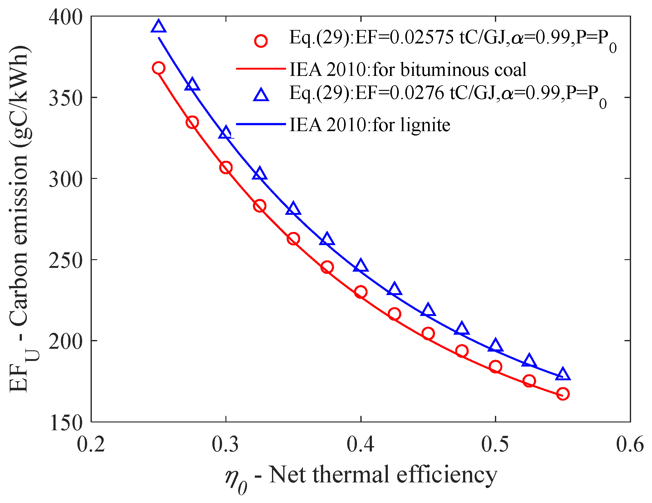
39A special case of Equation (29) can be obtained by assigning 1 to $\mathrm{P}/{\mathrm{P}}_0$ to show the dependence of carbon emission (${\mathrm{E}\mathrm{F}}_{\mathrm{U}}$) on unit efficiency (${\eta }_0$) at rated output. ${\mathrm{E}\mathrm{F}}_{\mathrm{U}}$ vs. ${\eta }_0$ was plotted scatteringly for a total of 13 data points in Figure 13. For comparison, the results of carbon emissions published by the International Energy Agency [22], which are in terms of specific CO₂ emissions originally, were converted to specific carbon emissions and plotted as a solid line in Figure 13. It can be seen that all data points of the predicted carbon emission from Equation (29) almost fall on the IEA lines, showing good agreement with each other.

6. Unit Study

A super thermal power unit of 1000 MW rated output, in routinely cyclic operation of increasing from half load at 05:30 to nearly full load at 08:00 and decreasing from full load at 20:30 to half load at 22:45, was chosen to estimate carbon emissions during cyclic operation under various of coals.

Carbon emission estimation was conducted through Equation (28) as well as through the input-output carbon balance approach. In the former, the carbon emission was estimated through the measurement of gross load ($\mathrm{P}$). Gross load is measured continuously in the Distributed Control System. Ash samples were compiled from the hoppers of the electrostatic precipitator to determine the coal oxidation rate ($\alpha$) by measuring the heat released from the ash in the Loss of Ignition (LOI) test. It shows that the value of the coal oxidation rate varied between 0.982 and 0.988 at different gross loads and could be taken as a constant value of 0.986. To calculate the standard coal consumption rate (${\mathrm{B}}_0$) at rated output, measurements of boiler efficiency, turbo-generator heat rate, and auxiliaries power consumption (${\mathrm{P}}_{\mathrm{A}0}$) at full load (${\mathrm{P}}_{\mathrm{G}0}$) were carried out in the acceptance test following the GB 10184-88 and GB 8117-87 procedures. Coal samples were collected from each operating feeder before the tube mill at a definite interval throughout the sampling period. Collected samples were mixed thoroughly to make a representative sample for the ultimate analysis, proximate analysis, and calorific value measurement. Sample preparation, ultimate and proximate analysis, and ash ignition test were conducted following the SAC/ISO procedure. The carbon emission was estimated using Equation (28), which is denoted as ${\mathrm{E}\mathrm{F}}_{\mathrm{U}1}$ and ${\mathrm{E}\mathrm{F}}_{\mathrm{U}2}$; ($\mathrm{E}\mathrm{F}$) is the carbon emission factor of firing coal computing from Equations (16) and (20), respectively.

For estimation through the input-output carbon balance method, carbon emission was computed from Equation (5), denoted as ${\mathrm{E}\mathrm{F}}_{\mathrm{U}3}$. The coal mass flow rate (m) is a summarization of all flow rates of the feeders in operation; $\left[\mathrm{C}\right]$ in Equation (5) is the carbon content on a basis; ${\mathrm{P}}_{\mathrm{N}}$ in Equation (5) is the net power generation calculated from Equation (7).

Table 8. Parameters used to estimate ${\mathrm{E}\mathrm{F}}_{\mathrm{U}}$ and estimate results.

Parameters	Results
${\mathrm{P}}_{\mathrm{G}0}$ MW	997.377
${\mathrm{B}}_0$ g/kWh	285.7
${\mathrm{P}}_{\mathrm{A}0}$ MW	45.08
$\alpha$	0.986
$\left[\mathrm{M}\right]$ %	12.37
$\left[\mathrm{A}\right]$ %	24.03
$\left[\mathrm{C}\right]$ %	51.53
$\left[\mathrm{H}\right]$ %	3.15
$\left[\mathrm{O}\right]$ %	7.45
$\left[\mathrm{N}\right]$ %	0.90
$\left[\mathrm{S}\mathrm{t}\right]$ %	0.57
$\left[\mathrm{F}\mathrm{C}\right]$ %	38.21
$\left[\mathrm{V}\right]$ %	25.39
NCV MJ/kg	19.65
GCV MJ/kg	20.58
Time averaged ${\mathrm{E}\mathrm{F}}_{\mathrm{U}1}$ g/kWh	223.7
Time averaged ${\mathrm{E}\mathrm{F}}_{\mathrm{U}2}$ g/kWh	225.4
Time averaged ${\mathrm{E}\mathrm{F}}_{\mathrm{U}3}$ g/kWh	232.7

summarizes all the parameters used to estimate EF_U from Equations (5) and (28).

Figure 14 plots the ${\mathrm{E}\mathrm{F}}_{\mathrm{U}1}$, ${\mathrm{E}\mathrm{F}}_{\mathrm{U}2}$, ${\mathrm{E}\mathrm{F}}_{\mathrm{U}3}$, m, and $\mathrm{P}$ profiles with time. As seen, gross load increases as time proceeds, accomplished by increasing the coal mass flow rate. Predictions of the carbon emission from Equation (28), i.e., ${\mathrm{E}\mathrm{F}}_{\mathrm{U}1}$ and ${\mathrm{E}\mathrm{F}}_{\mathrm{U}2}$, as well as that from Equation (5), i.e., ${\mathrm{E}\mathrm{F}}_{\mathrm{U}3}$, follow a similar trend of decreasing with time. However, the time average value of ${\mathrm{E}\mathrm{F}}_{\mathrm{U}3}$ is 232.7 g/kWh, while that of ${\mathrm{E}\mathrm{F}}_{\mathrm{U}1}$ and ${\mathrm{E}\mathrm{F}}_{\mathrm{U}2}$ are 223.7 g/kWh and 225.4 g/kWh, respectively. On average, predictions from Equation (5) give nearly 4% more carbon emission than that from Equation (28). This is due to the fact that Equation (28) is based on performance assessments, which implies a steady state operation at each data point of unit load, while Equation (5) is applied in a transient process in which both gross load and coal feed flow rate have been set to full automatic control mode to meet the requirement of the power grid, resulting in a substantial fluctuation of ${\mathrm{E}\mathrm{F}}_{\mathrm{U}3}$ predictions and more fuel consumption [42], with carbon emissions increasing accordingly.

To increase the use of more readily available coal, the unit combusted at least ten types of coal. The proximate analysis of three coals in conjunction with carbon emission factors estimated from Equation (20) is listed in

Table 9. Proximate analysis of firing coals and their carbon emission factors estimated from Equation (20).

Coal	$\left[\mathbf{M}\right]$ %	$\left[\mathbf{A}\right]$ %	$\left[\mathbf{F}\mathbf{C}\right]$ %	$\left[\mathbf{V}\mathbf{M}\right]$ %	$\left[\mathbf{S}\mathbf{t}\right]$ %	NCV MJ/kg	GCV MJ/kg	$\mathbf{E}\mathbf{F}$ kg/GJ NCV
Coal 1	19.00	13.49	43.30	24.21	0.45	20.11	21.19	26.96
Coal 2	9.40	26.65	37.74	26.21	0.58	19.93	20.83	25.77
Coal 3	10.00	27.47	31.93	30.60	2.06	19.92	20.85	24.50

. Carbon emissions were estimated using Equation (28) at various gross loads and types of coals. Figure 15 plots carbon emissions and gross load profiles with time. It indicates that at the same load, carbon emission when combusting coal 1 is on average 4.86% higher than coal 2 and that when combusting coal 2 is on average 4.90% higher than coal 3. As the gross load increases from approximately 56% to 91% rated output, carbon emission decreases by 5.4%, 5.9%, and 5.5% when combusting coal 1, coal 2, and coal 3, respectively. As the unit load decreases from 90% to 57% rated output, carbon emission increases by 5.5%, 5.3%, and 5.9% when combusting coal 1, coal 2, and coal 3, respectively.

The maximum difference in carbon emission is between the operating scenario of firing coal 3 at 900 MW load and that of firing coal 1 at 562 MW load; in the former operating scenario, carbon emission is 203.6 g/kWh, in the latter is 236.8 g/kWh; the relative increase is 16.3% including 10.0% due to coal variation and 6.3% due to load decrease. It is worth noting that the impact of firing coal on boiler efficiency is neglected. Actually, the high moisture content in coal 1 could induce a decrease in boiler efficiency due to heat loss of moisture vaporization and, therefore, an increase in both net heat rate and carbon emission. The increase in carbon emission attributable to coal variation would actually exceed 10% accordingly. Also, if the cyclic load range of the unit is expanded by 35% to 100% rated output, the increase in carbon emissions due to load decrease alone will reach nearly 17.44%, according to Figure 13. Thus, the maximum variation of carbon emissions attributed to the combined effect of firing coal and cycling load is at least 27.44% if the unit cycles at 35% to 100% rated output with coal normally varies in the present context.

7. Conclusions

Correlations of calorific value with ultimate analysis are very helpful in investigating the effect of elemental composition on the carbon emission factor of coal. Of the existing correlations, the Given correlation is noteworthy for both higher estimating accuracy and calculating the heating value of each component of coal individually. The Given correlation was revised by adding a new nitrogen term and using thermodynamic data from the latest JANAF tables in this work. The revised correlation has the highest estimation accuracy in terms of AAE as well as RMSE errors among all the correlations except the Mendeleev correlation.

The partial derivatives of the carbon emission factor of coal over $[\mathrm{C}$], $[\mathrm{H}$], $[\mathrm{O}$], $[\mathrm{N}$], $[\mathrm{S}$], $[\mathrm{A}$], and $[\mathrm{M}$] content were computed and averaged on a dataset of 247 coals, respectively. A correlation of the carbon emission factor with elemental composition was derived from the first-order Taylor series approximation. It showed that carbon emission factors (kg C/GJ NCV) rise by about 0.066, 0.161, 0.008, 0.034, and 0.004 kg C/GJ for each percentage increment of $[\mathrm{C}$], $[\mathrm{O}$], $[\mathrm{N}$], $[\mathrm{M}$], and $[\mathrm{A}$] content, respectively, and decline by 1.456 and 0.113 kg C/GJ for each respective percentage increment of H and S content. Based on the revised Given correlation, the O/C and H/C Molar ratio at the lowest carbon emission factor of coal was evaluated. It revealed that coals have the lowest carbon emission factor value of 22.73 to 22.92 kg C/GJ GCV at atomic O/C and H/C ratio range of 0.08 and 0.92 to 0.99, respectively. Stepwise linear regression removes the moisture term from the correlation of carbon emission factor (kg C/GJ GCV) with proximate analysis because the moisture considered in combustion products is of the same state as that in coal.

Net heat rates/thermal efficiencies of power thermal units at various load conditions were calculated from turbo-generator heat rates and boiler efficiencies in performance calculation sheets from the manufacturers. The varying nature of the net heat rate with load level is well expressed by a generic model derived from the exponential regression. The influence of firing coal and cyclic load on carbon emissions is captured with the derived correlation, which shows that at the load factor of 0.9, 0.8, 0.7, 0.6, 0.5, and 0.4, carbon emission increases 0.66%, 1.64%, 3.12%, 5.34%, 8.67%, and 13.68% compared to the full load, respectively. A case study in a thermal power unit with a rated output of 1000 MW shows that the total variation of carbon emission due to the combined effects of coal and cycling load could be 27.44% if the unit cycles at 35% to 100% rated output with coal normally varying in the present context.

In the end, one should be very careful to deploy Equation (25) to predict unit net heat rate in abnormal cases such as failure outage of HP heaters, significant low temperature of fresh steam, or putting desuperheating water of reheated steam into use during operation.

References

- Eser, P.; Singh, A. Effect of increased renewables generation on operation of thermal power plants. Appl. Energy 2016, 164, 723–732. [Google Scholar] [CrossRef]
- Yi, Y. China Renewable Energy Development Report, 1st ed.; China Renewable Energy Engineering Institute: Beijing, China, 2023; pp. 5–18. [Google Scholar]
- Mills, S.J. Integrating Intermittent Renewable Energy Technologies with Coal-Fired Power Plant; IEA Clean Coal Centre: London, UK, 2011; pp. 34–61. [Google Scholar]
- Habip, S.; Hikmet, E. The usage of renewable energy sources and its effects on GHG emission intensity of electricity generation in Turkey. Renew. Energy 2022, 192, 859–869. [Google Scholar]
- Gutiérrez, M.F.; Silva, R.A.D. Effects of wind intermittency on reduction of CO2 emissions: The case of the Spanish power system. Energy 2013, 61, 108–117. [Google Scholar] [CrossRef]
- Turconi, R.; Dwyer, C.O. Emissions from cycling of thermal power plants in electricity systems with high penetration of wind power: Life cycle assessment for Ireland. Appl. Energy 2014, 131, 1–8. [Google Scholar] [CrossRef]
- Mahlia, T.M.I.; Lim, J.Y. Methodology for implementing power plant efficiency standards for power generation: Potential emission reduction. Clean Technol. Environ. Policy 2018, 20, 309–327. [Google Scholar] [CrossRef]
- EFDB Emission Factor Database. Available online: http://www.ipcc-nggip.iges.or.jp/EFDB/main.php (accessed on 9 March 2023).
- Hong, B.D.; Slatick, E.R. Carbon dioxide emission factors of coal. Q. Coal Rep. 1994, 1–8. Available online: https://www.osti.gov/etdeweb/biblio/82283 (accessed on 9 March 2023).
- Chen, X.; Huang, J.; Yang, Q.; Nielsen, C.P.; Shi, D.; McElroy, M.B. Changing carbon content of Chinese coal and implications for emissions of CO2. J. Clean. Prod. 2018, 194, 150–157. [Google Scholar] [CrossRef]
- Suqin, J.; Zun, C. Committed CO2 emissions of China’s coal-fired power generators from 1993 to 2013. Energy Policy 2017, 104, 295–302. [Google Scholar]
- Zhu, L.; Dabo, G. Reduced carbon emission estimates from fossil fuel combustion and cement production in China. Nature 2015, 524, 335–340. [Google Scholar] [CrossRef]
- Sarkar, P.; Sahu, S.G. Revision of country specific NCVs and CEFs for all coal categories in Indiancontext and its impact on estimation of CO2 emission from coal combustion activities. Fuel 2019, 236, 461–467. [Google Scholar] [CrossRef]
- Jeffrey, C.Q.; Eric, M. Systematic error and uncertain carbon dioxide emissions from U.S. power plants. J. Air Waste Manag. Assoc. 2019, 69, 646–658. [Google Scholar] [CrossRef]
- Jeffrey, C.Q. Carbon dioxide emission tallies for 210 U.S. coal-fired power plants: A comparison of two accounting methods. J. Air Waste Manag. Assoc. 2014, 64, 73–79. [Google Scholar] [CrossRef]
- Katherinev, A.; Erict, S. Comparison of Two U.S. Power-Plant Carbon Dioxide Emissions Data Sets. Environ. Sci. Technol. 2008, 42, 5688–5693. [Google Scholar]
- Sakulpitakphon, T.; Hower, J.C. Predicted CO2 emissions from maceral concentrates of high volatile bituminous Kentucky and Illinois coals. Int. J. Coal Geol. 2003, 54, 185–192. [Google Scholar] [CrossRef]
- Winschel, R.A. The relationship of carbon dioxide emissions with coal rank and sulfur content. J. Air Waste Manag. Assoc. 1990, 40, 861–865. [Google Scholar] [CrossRef]
- Quick, J.C.; Glick, D.C. Carbon dioxide from coal combustion: Variation with rank of US coal. Fuel 2000, 79, 803–812. [Google Scholar] [CrossRef]
- Roy, J.; Sarkar, P. Predictive equations for CO2 emission factors for coal combustion, their applicability in a thermal power plant and subsequent assessment of uncertainty in CO2 estimation. Fuel 2009, 88, 792–798. [Google Scholar] [CrossRef]
- Dios, M.; Souto, J.A. Experimental development of CO2, SO2 and NOx emission factors for mixed lignite and subbituminous coal-fired power plant. Energy 2013, 53, 40–51. [Google Scholar] [CrossRef]
- International Energy Agency. Factors influencing power plant efficiency and emissions. In Measuring and Reporting Efficiency Performance and CO2 Emissions, 1st ed.; IEA Publ: Paris, France, 2010; pp. 34–35. [Google Scholar]
- Dong, Y.; Jiang, X. Coal power flexibility, energy efficiency and pollutant emissions implications in China: A plant-level analysis based on case units. Resour. Conserv. Recycl. 2018, 134, 184–195. [Google Scholar] [CrossRef]
- Akpan, P.U.; Fuls, W.F. Cycling of coal fired power plants: A generic CO2 emissions factor model for predicting CO2 emissions. Energy 2021, 214, 119026.1–119026.11. [Google Scholar] [CrossRef]
- Xuehua, Z.; Jeremy, S. Continuous emission monitoring systems at power plants in China: Improving SO2 emission measurement. Energy Policy 2011, 39, 7432–7438. [Google Scholar] [CrossRef]
- Eggleston, S.; Buendia, L. IPCC Guidelines for National Greenhouse Gas Inventories; Institute for Global Environmental Strategies (IGES): Hayama, Japan, 2006; Volume 1, pp. 6–8. [Google Scholar]
- DL/T 904-2004:30-32; National Development and Reform Commission of the PRC. Calculating Method of Economical and Technical Index for Thermal Power Plant. National Development and Reform Commission of the PRC: Beijing, China, 2004.
- Marek, S. Rank-dependent formation enthalpy of coal. Fuel 2013, 114, 2–9. [Google Scholar] [CrossRef]
- Maksimuk, Y.; Antonava, Z. Prediction of higher heating value based on elemental composition for lignin and other fuels. Fuel 2020, 263, 116727.1–116727.9. [Google Scholar] [CrossRef]
- Mott, R.A.; Spooner, C.E. The calorific value of carbon in coal: The Dulong relationship. Fuel 1940, 226–231, 242–251. [Google Scholar]
- Richards, A.P.; Haycock, D. A review of coal heating value correlations with application to coal char, tar, and other fuels. Fuel 2021, 283, 118942.1–118942.16. [Google Scholar] [CrossRef]
- Mason, D.M.; Gandhi, K.N. Formulas for calculating the calorific value of coal and coal chars: Development, tests, and uses. Fuel Process. Technol. 1983, 7, 11–22. [Google Scholar] [CrossRef]
- Given, P.H.; Weldon, D. Calculation of calorific values of coals from ultimate analyses: Theoretical geochemical implications theoretical geochemical implications. Fuel 1986, 65, 849–853. [Google Scholar] [CrossRef]
- Neavel, R.C.; Smith, S.E. Interrelationships between coal compositional parameters. Fuel 1986, 65, 312–320. [Google Scholar] [CrossRef]
- Channiwala, S.A.; Parikh, P.P. A unified correlation for estimating HHV of solid, liquid and gaseous fuels. Fuel 2002, 81, 1051–1063. [Google Scholar] [CrossRef]
- Singh, P.K.; Kakati, M.C. New models for prediction of specific energy of coal. Fuel 1994, 73, 301–303. [Google Scholar] [CrossRef]
- King, T.M.; Attwood, D.H. Predicting specific energies for brown coal samples. Fuel 1980, 59, 602–603. [Google Scholar] [CrossRef]
- Ringen, S.; Lanum, J. Calculating heating values from elemental compositions of fossil fuels. Fuel 1979, 58, 69–71. [Google Scholar] [CrossRef]
- Mathews, J.P.; Krishnamoorthy, V. A review of the correlations of coal properties with elemental composition. Fuel Process. Technol. 2014, 121, 104–113. [Google Scholar] [CrossRef]
- Mastalerz, M.; Drobniak, A. Variations in CO2 emissions from Pennsylvanian coals of the eastern part of the Illinois Basin. Int. J. Coal Geol. 2013, 108, 10–17. [Google Scholar] [CrossRef]
- Quick, J.C.; Brill, T. Provincial variation of carbon emissions from bituminous coal: Influence of inertinite and other factors. Int. J. Coal Geol. 2002, 49, 263–275. [Google Scholar] [CrossRef]
- Neshumayev, D.; Rummel, L. Power plant fuel consumption rate during load cycling. Appl. Energy 2018, 224, 124–135. [Google Scholar] [CrossRef]
Figure 1.
Ultimate analysis data arranged in a stacked area.
Figure 2.
Efficiency performance at various loads: (a) boiler efficiency; (b) heat rate of turbo-generator.
Figure 3.
Determination of and in Equation (13) with least-squares algorithm. , .
Figure 4.
Heat contribution from each component is arranged in a stacked area.
Figure 5.
Prediction of carbon emission factor from Equation (16) vs. observed values.
Figure 6.
VAN Krevelen plot and the lowest carbon emission factor.
Figure 7.
Prediction of carbon emission factor from Equations (19) and (20) vs. observed values.
Figure 8.
Ratios of auxiliary power fraction vs. load factor.
Figure 9.
Efficiency performance at various loads: (a) Coal consumption rate for net power production; (b) Net thermal efficiency.
Figure 10.
and at various load factors: (a) ; (b) .
Figure 11.
Carbon emissions at various loads.
Figure 12.
Increases of carbon emission relative to full load in PS and [
24].
Figure 13.
Special scatter plot from Equation (29) and IEA lines [
22].
Figure 14.
The , , , m, and profiles with time.