Article

A Reduced Stochastic Data-Driven Approach to Modelling and Generating Vertical Ground Reaction Forces During Running

by
Guillermo Fernández
1,
José María García-Terán
1,
Álvaro Iglesias-Pordomingo
1,
César Peláez-Rodríguez
2,
Antolin Lorenzana
1 and
Alvaro Magdaleno
1,*
1
ITAP-EII, Universidad de Valladolid, Pº del Cauce 59, 47011 Valladolid, Castilla y León, Spain
2
Departamento de Teoría de la Señal y Comunicaciones, Universidad de Alcalá, Campus Universitario, Ctra. Madrid-Barcelona, km 33, 600, 28805 Alcalá de Henares, Madrid, Spain
*
Author to whom correspondence should be addressed.
Modelling 2025, 6(4), 144; https://doi.org/10.3390/modelling6040144
Submission received: 8 October 2025 / Revised: 30 October 2025 / Accepted: 3 November 2025 / Published: 6 November 2025

Abstract

This work presents a time-domain approach for characterizing the Ground Reaction Forces (GRFs) exerted by a pedestrian during running. It is focused on the vertical component, but the methodology is adaptable to other components or activities. The approach is developed from a statistical perspective. It relies on experimentally measured force-time series obtained from a healthy male pedestrian at eight step frequencies ranging from 130 to 200 steps/min. These data are subsequently used to build a stochastic data-driven model. The model is composed of multivariate normal distributions which represent the step patterns of each foot independently, capturing potential disparities between them. Additional univariate normal distributions represent the step scaling and the aerial phase, the latter with both feet off the ground. A dimensionality reduction procedure is also implemented to retain the essential geometric features of the steps using a sufficient set of random variables. This approach accounts for the intrinsic variability of running gait by assuming normality in the variables, validated through state-of-the-art statistical tests (Henze-Zirkler and Shapiro-Wilk) and the Box-Cox transformation. It enables the generation of virtual GRFs using pseudo-random numbers from the normal distributions. Results demonstrate strong agreement between virtual and experimental data. The virtual time signals reproduce the stochastic behavior, and their frequency content is also captured with deviations below 4.5%, most of them below 2%. This confirms that the method effectively models the inherent stochastic nature of running human gait.

1. Introduction

Human locomotion is a complex process involving various psychomotor capabilities (e.g., balance, strength, emotional state) that enable movement by overcoming obstacles and resistance from gravity and air. Depending on the field of study, locomotion exhibits different characteristics [1]. In particular, human gait is primarily divided into walking and running, where the forces exerted on the ground by the pedestrian, known as Ground Reaction Forces (GRFs), play a crucial role [2]. These forces have three components: anteroposterior (forward movement), mediolateral (transverse sway oscillations), and vertical (the most significant). Other actions of interest, though without relevant displacement, include jumping and bouncing—the latter without losing ground contact—where the vertical component is almost the only relevant one. Conceptually similar, GRFs and their patterns vary depending on the motor activity, requiring an individualized approach, while maintaining common general rules. Specifically, the study presented in this paper focuses on the vertical GRFs of a pedestrian during running.
The complexity of GRFs arises from their nondeterministic nature, where a force generated during one step is not identical to others but is statistically similar [3]. Considering randomness is key to developing accurate models for the simulation and prediction of the aforementioned forces. These models are essential in such fields as structural engineering, biomechanics, and physiotherapy. In the first, the time and frequency analysis of vertical GRFs, as one of the main sources of dynamic excitation, is crucial for preventing serviceability issues in pedestrian structures. The second allows the interaction between body segments during gait to be simulated and movement-related risks [4,5] to be assessed. Finally, in physiotherapy, GRFs can be used in diagnosing and treating gait disorders [6]. Reduced models are of great interest because they use the minimum necessary variables and parameters, optimizing efficiency while maintaining accuracy and applicability.
Several studies, some of which are related to the reproduction of human loads, have developed models to simulate GRFs in both time and frequency domains [3]. These algorithms can be based on periodic analytic functions fitted to experimental data—a deterministic approach with Fourier decomposition regarding amplitudes, frequencies, and phases [7]—or on stochastic models that assume near-periodic signals, addressing the inherent variability of gait. In this context, Racic et al. have proposed data-driven algorithms (using data collected at constant step frequencies) based on Gaussian functions to preserve the shape and randomness of GRFs during walking [8], running [9], jumping [10], and bouncing [11]. These combined with auto-spectral densities for gait cycle duration and linear regressions that account for force magnitude scaling. Autoregressive models have been dismissed due to their inefficiency [12]. Other authors, such as Li et al., propose a similar methodology for jumping, but with cycle times modelled as normal random variables [13]. Alternatively, Chen et al. model jumps using wavelet transforms [14], while Pancaldi et al. combine classical Fourier decomposition with univariate and multivariate normal distributions, obtaining Gaussian Mixtures and Markov random walks for the generation of virtual gaits [15,16,17]. García-Diéguez et al. stochastically reproduced vertical GRFs at variable speed [18], providing an alternative approach to fixed step frequencies. All of these techniques have resulted in robust algorithms that simulate different types of GRFs in time and also reproduce their frequency content (up to several harmonics).
Other approaches include nonlinear time physical models. Unlike mathematical-statistical techniques, these indirectly reproduce GRFs from simple mechanisms, where parameter tuning and numerical resolution allow for the simulation of forces. In this regard, Cacho and Lorenzana propose a double inverted pendulum to model a pedestrian walking on a coupled vibrating structure [19], a study similar to that conducted by Lin et al. but on a rigid floor [20], the 3D model by Liang et al. [21], and the modified autonomous oscillator from Rayleigh, Van der Pol, and Duffing, forms developed by Kumar et al. [22]. Alternatively, Xiang et al. present a 55-degree-of-freedom human model for the numerical prediction of GRFs during walking (among other kinematic magnitudes) [23], while Wang et al. develop a method for identifying the physical parameters of a pedestrian’s mass-spring-damper system by means of a particle filter algorithm [24]. Other studies with similar models reproduce GRFs during running, such as those by Masters et al. [25] and Zanetti et al. [26], the latter with an interesting approach based on modal analysis and the superposition of the actions present in a running GRF.
Finally, other techniques use wearable devices, such as Inertial Measurement Units, to record human body kinematics, along with correlation and Machine Learning models for the indirect estimation of GRFs [27,28,29,30]. A literature review on this subject has been compiled by Ancillao et al. [31].
As indicated, the literature offers a wide range of models to characterize GRFs. Nevertheless, although many of the proposed works are comprehensive, some important limitations remain. On the one hand, stochastic models, while capturing the inherent variability of gait, do not explicitly account for the potential asymmetry between the forces exerted by each individual foot, which may have an influence in the resultant action. Furthermore, most datasets are constrained to laboratory environments, relying on force plates or treadmills and making continuous measurements difficult [32,33]. On the other hand, nonlinear physical models often treat GRFs as deterministic and symmetric actions, an assumption that limits their capability for a rigorous modelling of gait. Moreover, they do not consider reducing the model to the minimum necessary variables and parameters either. These shortcomings highlight the need for newer stochastic approaches capable of combining individual foot modelling with randomness-preserving techniques.
Considering all of the above, this paper proposes a time-domain stochastic data-driven model to characterize and generate virtual GRFs of a particular pedestrian while running. An improved continuation of related studies by the authors regarding the walking action [34,35], its contributions with respect to other works in the state of the art reside in the following points:
  • The development of a time-domain stochastic model based on experimental data collected with a pair of instrumented insoles at different step frequencies, avoiding any too constrained laboratory setting;
  • The independent modelling of each foot’s GRF, capturing gait’s inherent variability across feet. In this regard, vertical GRFs were analyzed, and the resultant total action was evaluated at the end. The approach could be extended to other force components with adjustments not addressed here;
  • The use of a rigorous statistical procedure to model the aforementioned pedestrian’s running GRFs without resorting to deterministic approaches or purely mathematical frameworks;
  • The implementation of a dimensionality reduction algorithm that preserves the main GRF characteristics in the virtual signals, using the minimum necessary variables and parameters through an optimization workflow.
Additionally, the stochastic model separately considers the time scaling of steps and aerial times, both modelled as normal random variables, as well as the pattern of the forces, which follows a time-independent multivariate normal distribution by means of the covariance matrix computation. Under the normality assumption, verified through statistical tests, the algorithm generates virtual gaits from pseudo-random numbers.
The document is structured as follows: this first section introduces the topic and presents a state-of-the-art review. Next, Section 2 details the Materials and Methods used in the study, covering terminology, the adopted approach for the experimental measurement of running GRFs, and the full development of the stochastic model and its algorithms. Section 3 presents the main results, while Section 4 and Section 5 are dedicated, respectively, to the analysis and discussion of the results and the main conclusions.

2. Materials and Methods

2.1. Running Human Gait and Terminology

Before addressing the methodology, key concepts and terminology related to running human gait are briefly introduced in the present section. As stated in the Introduction, running is a complex process involving multiple human abilities, making each step unique. However, certain general characteristics are common across people.
Running is a near periodic activity consisting of four phases, collectively known as the gait cycle, which can also be defined as two successive footfalls (stride to stride) or any other consecutive similar events. Figure 1 illustrates these four phases and presents an example of the vertical GRFs exerted on the ground, which can vary slightly in shape depending on the runner’s specific running style (mid-frontfoot running pattern in Figure 1a and rearfoot—heel strike in Figure 1b). During the first and third phases, known as aerial, neither foot contacts the ground. The first begins with right toe-off and ends with left foot contact (duration t R L ), while the third follows the opposite pattern ( t L R ). In between, the second and fourth stance phases involve continuous ground contact, with the left and right foot solely generating the step force, respectively.
As observed in the GRFs for both feet and running styles, a maximum, known as the Active Peak (AP), occurs during each step. In rearfoot runners, an initial, smaller peak can appear just after the heel strikes the ground, referred to as the Impact Peak (IP), during which a significant fraction of the body weight (BW) is loaded on that foot for a very short time. Regarding the resultant force, which represents the effective force applied to the ground by the runner, it is composed of the individual GRFs from each foot, separated by the aerial phases mentioned.

2.2. Experimental GRF Dataset: Measurement and Testing Protocol

In this study, a pair of instrumented insoles placed inside the footwear were used to measure the experimental vertical GRFs [36,37]. Various alternatives have been employed by other authors, such as force plates, which do not allow continuous GRF measurement during prolonged running, or instrumented treadmills [32,33]. While these methods are professional and precise, they are expensive, challenging to calibrate, and limit experimental data gathering to laboratory settings. In this regard, Novel GmbH Loadsol® insoles were used [38] (Figure 2a). These devices have been validated by other authors, demonstrating good test-retest reliability and highlighting their suitability for gait analysis beyond laboratory settings [39,40]. They measure the total vertical force exerted by the foot using a 99-capacitive sensor grid and transit data via Bluetooth to a smartphone at a sampling rate ( f s ) of 100 S/s.
Experimental GRFs were recorded using the aforementioned insoles (Figure 2b), worn by a 55-year-old healthy male inside sports footwear (93.3 kg, measured on a common medical scale, with a height of 177 cm). The pedestrian ran at eight different step frequencies, ranging from 130 to 200 steps/min (2.17 to 3.33 Hz), assisted by a digital portable metronome. Trials were carried out on a 100 m straight rigid path with a flat, regular and obstacle-free surface. The experiments were performed under standard outdoor conditions, with appropriate ambient temperature for physical activity. Since the insoles are synchronized, the i-th elements from both left-right signals are assumed to occur simultaneously, and two data vectors were obtained. The testing protocol involved calibrating the insoles individually at the start of the first trial (130 steps/min) using the pedestrian’s BW, with the calibration assumed to remain stable throughout all experiments. Data recording began at the start of each trial, was stopped upon reaching the end of the path, and saved. After a 2-min rest, the step frequency was increased by 10 steps/min, and another trial was performed. Once all the data had been saved, a dataset was created, along with the algorithms presented in the following sections [41].

2.3. Time Vector Data Processing

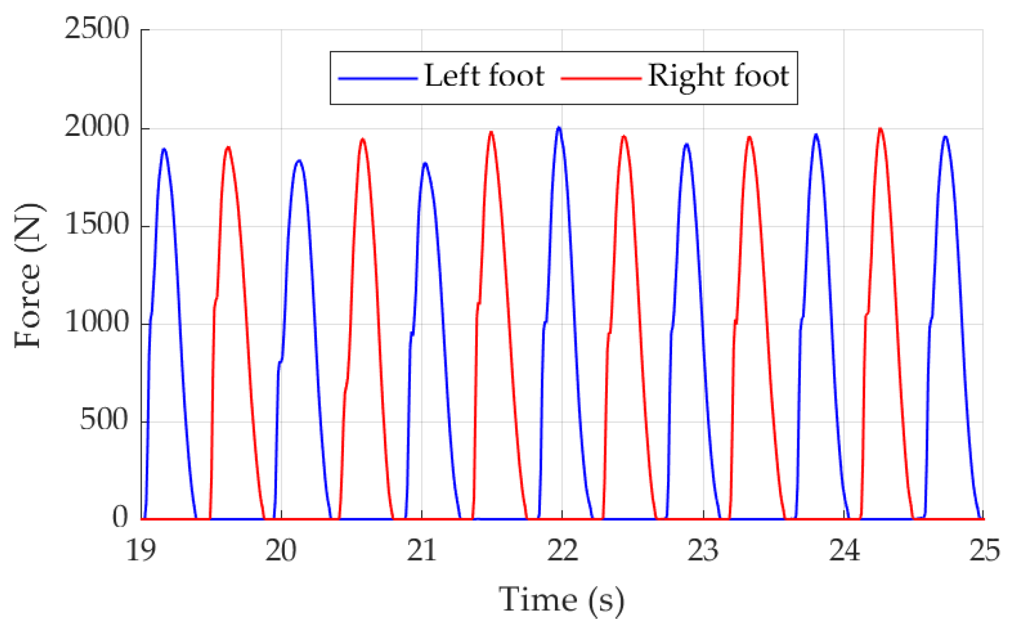
The force, time-synchronized vectors exerted by each foot at each step frequency were processed independently. Relevant data were first selected by manually defining a time interval t m i n ,   t m a x , discarding any values outside it, which may have contained irrelevant information for the model to be obtained. The final data arrays should retain as many consecutive steps as possible for subsequent automated processing. Figure 3 shows an example of both measured GRFs signals at 130 steps/min. Additional preprocessing, such as detrending or filtering could have been applied if needed. Once the final experimental vectors had been prepared, step (stance) samples were created through detection, isolation, and rescaling, by the methods explained in the following subsections, adapted from the ones presented in [34].

2.3.1. Step Detection Algorithm

Steps were first detected using the following algorithm. A sliding window w k   =   w 1 , , w a of width a   =   3 points was applied along each force vector to determine the beginning and end of each step. This detection relied on fundamental conditions related to the shape of the GRF, including its rising and falling edges during the stance phase, as illustrated in Figure 4. Window’s width a was chosen to ensure a robust step detection: using more than two points allows the proper meeting of the conditions explained below, while keeping the sliding window small avoids including samples that could distort the rising and falling edges of the GRFs. Consequently, a step began when the condition in Equation (1) (rising edge) was met, provided an auxiliary flag was previously false.
F > F t h d F d t F k + 1 F k t k + 1 t k > 0 k = 1 a 1 f l a g = F a l s e f l a g = T r u e w 1 = t 1 , F 1
The flag was then set to true, and the first point ( w 1 ) in the sliding window exceeding the threshold F t h was stored as the step start, reducing false detections caused by Loadsol® insole noise. Note that F t h is required in order to avoid issues related to noise around 0 N, mainly due to sensor noise. The value of this threshold should be higher than the sensor noise but small enough to minimize the loss of samples as possible at the start and end of the detected steps. In this regard, a value of 20 N (approx. 1% of the maximum GRF) was used, as it had been proven effective in previous works [34]. Similarly, when the flag was true and Equation (2) held (falling edge), the step ending was detected as the first point falling bellow F t h (last w 3 sample). This process was conducted for each foot’s GRF time series independently.
F < F t h d F d t F k + 1 F k t k + 1 t k < 0 k = 1 a 1 f l a g = T r u e f l a g = F a l s e w a = t a , F a

2.3.2. Step Duration Estimation: First Outlier Removal

Once detected and isolated, steps were extrapolated at their beginning and end using the corresponding points w 1 and w 3 to improve duration estimation, due to the influence of the threshold F t h on the start and end detections. Linear extrapolations were applied using sliding windows, extending steps to 0 N (Figure 4). Alternative methods may have failed to reach 0 N and do not improve approximations. Step estimated duration points were then calculated for each foot using Equation (3), where time estimations are denoted with *. After extrapolation, the number of f s points ( N f , j ) per step increases by two. Let m 0 be the initial sample size for each foot’s step count.
δ j t end , j t 1 ,     N f , j = N f , j + 2             with   j = 1,2 , , m 0
A first outlier removal stage was performed based on step duration. Since the model to be obtained must represent the set of steps that statistically characterize the pedestrian’s running action, the first ( Q 1 ) and third ( Q 3 ) quartiles and the Interquartile Range (IQR) were computed under the assumption that step duration δ behaved as a random variable with m 0 observations. Any steps with a duration outside the interval defined by Equation (4) were discarded, reducing the step sample size of each foot to m 1 .
IQR = Q 3 Q 1 ,           Outlier   if :     δ j Q 1 1.5 IQR ,   Q 3 + 1.5 IQR
Scaling factors η were derived in Equation (5) as the inverse of δ for subsequent analysis. The full sets of t 1 and t end values, without any removal in this case, were also saved for the aerial time characterization in Section 2.3.4.
η j = 1 δ j   with   j = 1,2 , , m 1

2.3.3. Step Rescaling and Geometric Characteristics: Second Outlier Removal

Final step samples were determined after rescaling and a second outlier removal stage based on geometric GRF characteristics. With the scaling factors computed to preserve duration information, each step’s extrapolated time vector was mapped to the range 0,1 using Equation (6), yielding a set of rescaled timestamps τ . After this task, another force rescaling to the pedestrian’s BW (reported in Section 2.2) was also conducted.
τ i j = t t 1 , j t end , j t 1 , j 0,1           with   i = 1,2 , , N f , j j = 1,2 , , m 1
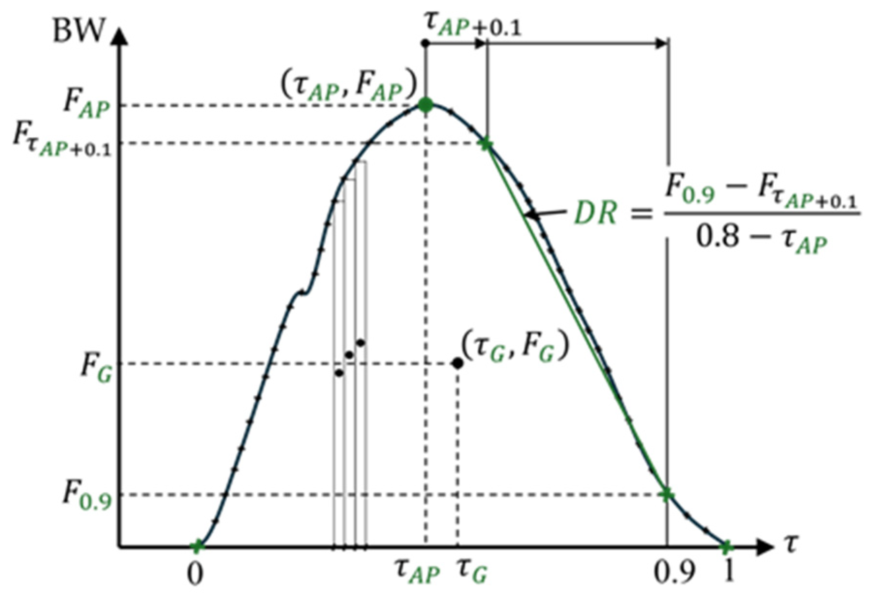
Geometric characteristics were determined by obtaining the values of three step pattern-related variables, also assumed to be random as δ . These variables were the AP (as seen in Figure 1), the Decay Rate (DR) and the GRF area centroid (G). A scheme is provided in Figure 5. The AP was computed as the GRF maximum and the corresponding instant ( τ AP ) at which it occurred, following Equation (7).
AP j = max F i ,       with     i = 1,2 , , N f , j ,     τ AP , F AP j           with   j = 1,2 , , m 1
DR represents the rate at which the GRF attenuates during stance after AP has been reached. It was determined using Equation (8), with the aid of an augmented set of fixed, 200 values to better identify the points ( τ AP + 0.1 , F AP + 0.1 ) and ( τ 0.9 , F 0.9 ) , by means of cubic Hermite interpolation. This was done following works on the performance of the Loadsol® performance [38,39], which suggest that 100 S/s is enough for precise measurements, but such variables as DR may require a refined calculation.
DR j = F 0.9 F τ AP + 0.1 0.8 τ AP     in   τ i j           with   i = 1,2 , , 200 j = 1,2 , , m 1
The third variable G represents the centroid of the area under the GRF curve, and corresponds to the energy involved during each foot’s step. It was calculated through numerical integration following the expressions of Equations (9) and (10) to determine τ G and F G , both represented by the generic symbol ϕ .
A i = τ i + 1 τ i F i + 1 F i ϕ ¯ i = 1 2 ϕ i + ϕ i + 1     with   i = 1,2 , , N f , j 1
ϕ j = A ϕ ¯ d A A d A i = 1 N f 1 ϕ ¯ i A i i = 1 N f 1 A i ,     τ G , F G j   with   j = 1,2 , , m 1
After the three geometric variables were computed, defining the step rescaled pattern ( m 1 observations per random variable sample), the second outlier removal stage was conducted. These samples were grouped into three subsets I X . Applying the IQR method (as for δ ), outliers in each subset were flagged as true. Using the step identifier j , the intersection of rescaled steps without any outlier was obtained (false subset values), discarding those that contained at least one atypical observation. These were thus excluded from the final step sample of size m from now on. Equation (11) formally expresses this.
I X False = j   |   X j = False ,     with   j = 1,2 , , m 1 ,     I False = I AP False I DR False I G False I False = m  
The whole process followed in this section was applied to the GRF dataset in Section 2.2. The number of statistically relevant steps is given in Table 1 for each foot and step frequency after each outlier removal stage.

2.3.4. Aerial Time Characterization

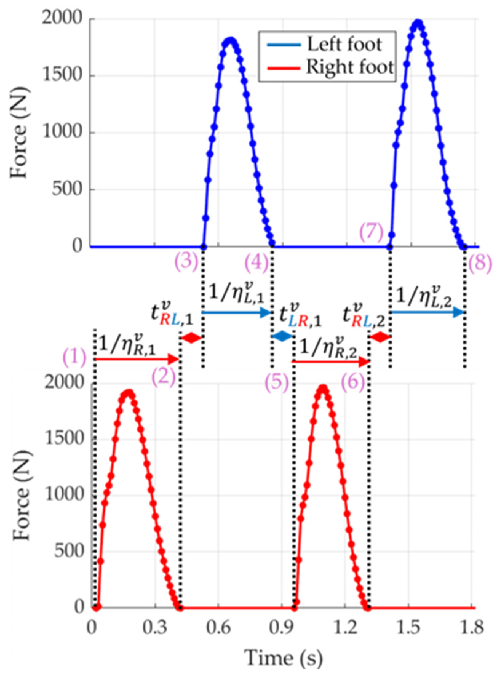
Based solely on their estimated durations, steps from each foot’s GRF time series do not represent how they concatenate over time to provide the signals shown in Figure 3, directly affecting the frequency content of the resultant GRF. To address this, start t 1 and end times t end —without considering the outlier nature of the steps they belonged to, already addressed previously—were used to estimate the aerial times, as defined in Section 2.1. Depending on the order in which the feet lost and regained ground contact (LR or RL), aerial time samples were obtained by means of Equation (12).
t L R , p = t 1 , R , p t end , L , p           with   p = 1,2 , , m 0 , L R t R L , p = t 1 , L , p t end , R , p           with   p = 1,2 , , m 0 , R L
Since t L R and t R L are part of gait’s random nature as they vary over time, only statistically significant values were of interest. The IQR method was again applied to discard outliers. Table 2 shows the final aerial time samples of size m 1 , L R and m 1 , R L .

2.4. Step Pattern Description Reduction

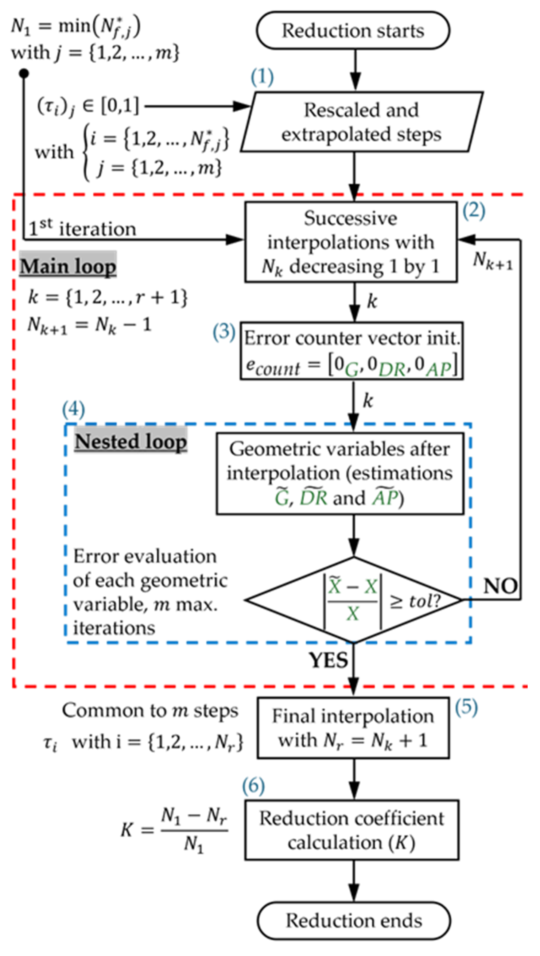
After addressing the methodology for step detection, isolation, rescaling, geometric and aerial time characterization, this section presents an algorithm implemented to reduce the geometric description while preserving key information for stochastic modelling. This improves the efficiency by using a reduced set of data that is sufficient for accurate replication. In this regard, the rescaled steps were resampled to a reduced set of equally spaced τ , F points according to the algorithm described in Figure 6. Taking the final samples of size m obtained in Section 2.3.3 as input, as well as their associated geometric variables after applying Equation (11), the workflow began by evaluating, for each step frequency and foot sample, the minimum number of points associated with the insoles f s , N 1 , from the varying N f , j values given in Section 2.3.2.
Through the main loop’s successively reduced cubic Hermite interpolation to N k points, new values of AP, DR, and G were estimated, denoted as X ~ for each variable. Shape preservation is achieved via C 1 continuity, interpolating both the steps up to their first derivative. Operating within the nested loop in Figure 6, which is detailed in Figure 7, the error counter vector ( e count ) accumulated the total number of failed variables estimations, based on their relative error and tolerances tol 1 ( F ) and tol 2 ( τ ), fixed at 5% and 15%, respectively. When the total number of out-of-tolerance estimations for any geometric variable reached or exceeded 10% of the sample size for a given foot and step frequency, the process was terminated to preserve accuracy. These tolerances values are chosen based on data inspection to ensure the finding of a reduced set of variables that faithfully represented the original experimental measurements. The specific choices balance data variability. Naturally, with other datasets, these tolerance values may need to be adjusted, while the overall pattern description reduction workflow remains totally applicable.
Considering the previous remarks, the pattern was considered sufficiently processed for reliable use. Finally, N r values were obtained and used to interpolate the GRFs to the final τ , F points uniformly. Table 3 shows these values and the corresponding K reduction coefficients, up to more than 60%.

2.5. Vertical GRFs Stochastic Model

Using the final processed data samples obtained in the previous sections, the stochastic model of the pedestrian’s vertical running GRFs for their virtual generation was constructed, under the assumption that the random variables involved followed normal distributions, assessed through statistical tests. Samples were then split into random subsets of 50 % for modelling (stm.) and 50 % for testing and validation (val.) after virtual GRF generation (Section 2.6). The model was built, and was composed of (including the runner’s BW):
  • Univariate normal distributions of each foot’s stm. step scaling factors random subsets, denoted as N μ η L stm , σ η L stm and N μ η R stm , σ η R stm ;
  • Univariate normal distributions of the stm. aerial times random subsets, denoted as N μ t L R   stm , σ t L R stm and N μ t R L stm , σ t R L stm ;
  • Two mean vectors, μ L stm and μ R stm , and their unbiased covariance matrices, S L stm and S R stm . These were obtained from computing the subset, centered, and rescaled GRF matrices F c stm in Equation (13) and applying the expression given in Equation (14), where x stands for round x . This accounted for each foot’s step pattern after its description had been reduced in Section 2.4. Each of the corresponding N r interpolation points was assumed to follow a normal distribution, with all the τ , F points collectively following multivariate normal distributions, denoted as N μ L stm , S L stm and N μ R stm , S R stm .
F c stm = I 2 m 1 1 T F 1 i F 1 N r F m / 2 i F m / 2 N r
S stm = 1 m 2 1 F c stm T F c stm
The total number of variables ( T V ) that made up the model, as well as the corresponding total number of parameters ( T P ), are given in Equation (15). Each scaling factor and aerial time represent a single normal random variable with two associated parameters, μ and σ , leading to a fixed total of 4 variables and 9 parameters, including the BW. Since the size of each step pattern model is given by the obtained reduced number of interpolation points N r in Section 2.4, an additional N r , L + N r , R random variables are introduced (left and right feet). The minimum number of a single foot’s unique parameters associated with these variables is N r N r + 1 / 2 , as the covariance matrix is square and symmetric, and each variable of the multivariate distribution has a mean (all gathered together in mean vectors of length N r ). Taking this into account, if an unnecessary number of points had been used (significantly higher than the values in Table 3), a much greater T P would have been obtained, resulting in inefficiency due to quadratic dependencies.
T V = 4 + N r , L + N r , R T P = 9 + 1 2 N r , L 2 + N r , R 2 + N r , L + N r , R

2.5.1. Step Pattern Multivariate Normality

Step pattern sample multivariate normality assumptions were checked with the Henze-Zirkler (HZK) test [42,43]. This test was chosen since it is one of the simplest and most robust for multivariate normality checking. However, it relies on the inversion of the covariance matrix following the Mahalanobis distance computation. In this regard, the sample covariance matrix S must be non-singular, i.e., full rank. Consequently, to preserve variability, a sample GRF centered submatrix F ~ c R m × N r 2 was derived for this task, in the same form as the one defined by Equation (13), but excluding the first and last null variance columns related to the extrapolated 0 BW value for both initial and final points obtained in Section 2.3.2. After performing Principal Component Analysis (PCA) [44] to explain, at least, 95% of the data variability in a reduced-dimensional space of d uncorrelated principal components (PCs), the test was executed for each sample of steps, foot, and step frequency. Table 4 indicates the corresponding HZK p-values and d PCs. Significance level was set at α = 0.05 .
Since the first d PCs explained sufficient variability via linear combinations of the original variables, multivariate normality could be assessed. PCA minimized the variables/observations ratio to avoid potential singularities related to interpolation points, essential for stochastic modelling but problematic for testing. The test suggested that the majority of samples were adequately modelled by a multivariate normal distribution (p-value >   α , accept null hypothesis), although a slight deviation was observed at 200 steps/min right steps, where p fell below α (null hypothesis rejection).

2.5.2. Scaling Factors and Aerial Times Univariate Normality

Scaling factors and aerial times samples were tested for univariate normality using the Shapiro-Wilk (SW) test [45,46], the most powerful statistical test for this task applied to the final sample sizes reported in Table 1 (m) and Table 2 ( m 1 , L R or m 1 , R L ). Specifically, stm. random subsets belonging to samples that failed to pass the SW test were transformed using the Box-Cox transformation [47], as given by Equation (16).
x x λ = x λ 1 λ ,           i f   λ 0 ln x ,           i f   λ = 0  
The corresponding λ factor was obtained by solving the corresponding Maximum Likelihood Estimation problem (MLE) [48] and subsequently saved. Then, it was used to reverse the transformation using the inverse Box-Cox form in Equation (17), thereby restoring the true data scaling of the virtual GRFs to be generated.
x 1 λ = exp ln 1 + λ x λ λ ,           i f   λ 0 exp x λ ,           i f   λ = 0  
An example of this procedure is shown in Figure 8, where scaling factors and aerial times at 140 steps/min were tested for normality. Histograms were plotted with bins adjusted following Sturges’ rule [49]. Since η L and η R failed to pass the test (p-value <   α , null hypothesis rejection), their stm. random subsets were transformed using Equation (16), and the SW test was reapplied (Figure 8a,d), achieving normal behavior ( p λ stm ). The corresponding λ factors were saved. The remaining variables, η R (Figure 8b) and t L R (Figure 8c), exhibited normal behavior since the beginning, requiring no transformation.

2.6. Virtual GRF Generation

With the stochastic model built in the previous section, the virtual GRF generation was divided into two main stages, which are introduced below and explained in the following paragraphs:
  • Virtual step generation: virtual left and right rescaled steps were generated using their stm. multivariate normal distributions. Each virtual step was then rescaled in time by means of virtual scaling factors η v , drawn from their respective univariate normal distributions;
  • Time concatenation: the aforementioned steps, in their original units of time(s) and force (N), were sequentially concatenated with the aid of virtual aerial times. A final common interpolation was performed to replicate the insoles sampling rate.
In this regard, the first stage started by generating a set of N g , L + N g , R virtual steps, N g , L for the left and N g , R for the right foot, approximately equaling the corresponding val. subset sizes. They were obtained by means of a multivariate pseudo-random number generation algorithm, making use of the N μ L stm , S L stm and N μ R stm , S R stm distributions defined in Section 2.5. In this work, the MATLAB® R2024b mvnrnd() algorithm was executed [50], since it is prepared to deal with the singularities present in the S stm matrices. Note that the virtual steps N r points were generated simultaneously, which was the reason for employing a multivariate distribution and a covariance approach [51,52]. If univariate distributions had been used for step pattern modelling, unrealistic noise would have arisen due to each virtual random value deviating from the model’s mean vector μ stm , independently of neighboring points. This is depicted in Figure 9 for a single left virtual step at 130 steps/min, with augmented interpolation only for visualization purposes.
As a consequence of how the stochastic model had been obtained, the virtual steps were then rescaled in time and BW, covering the range given in Equation (6). To address this, N g , L and N g , R pseudo-random virtual scaling factors ( η v ) were generated using the corresponding univariate normal distributions N μ L stm , σ L stm and N μ R stm , σ R stm for each foot individually. When normalization had been required through the Box-Cox transformation in Equation (16), λ factors were used to recover the scale and behavior of η v by applying the inverse transformation given in Equation (17). Consequently, a statistically similar step duration to the experimental one was obtained, and the BW was finally used to recover the GRF values in N as the final task prior to step concatenation.
Eventually, the second and final stage can be carried out. To proceed with this task, N g , L R and N g , R L (val. random subset sizes) pseudo-random virtual aerial times were generated through their normal distributions: N μ L R stm , σ L R stm and N μ R L stm , σ R L stm . This provided a way to account for both the LR and RL aerial phases in a separate, statistically similar way to the experimental expected values estimated in Section 2.3.4. Inversion of the Box-Cox transformation when needed was conducted accordingly as with η v . Virtual aerial times ( t L R v and t R L v ) were then used to assign the starting time for each virtual step based on the time at which the previous step ended. This process was repeated until 2 N g steps ( N g of each foot, N g = m i n ( N g , L , N g , R ) ) had been concatenated. Since each step had a different time increment and each pattern model could be made up of a different number of N r points (Section 2.4), both time-synchronized virtual GRF signals were resampled simultaneously. Cubic Hermite interpolation was used, as in previous sections, and the final time increment was adjusted to replicate the insoles sampling rate f s (100 S/s). An example of step concatenation is depicted in Figure 10 at 130 steps/min.
The full methodology described in the paper is summarized in Figure 11, with sections and subsections references for further details.

3. Results

This section presents the main results obtained after systematically applying the full methodology described in Section 2 to the pedestrian’s GRF time series at different step frequencies. It is important to note that some preliminary results and key data features that justify the methodology and its algorithms have already been presented, serving as a complement to the final results reported here. These mainly include the building of the stochastic models, which relies on the appropriate, outlier-free selection of both the stm. and val. random subsets (Section 2.3 and Section 2.5, Table 1 and Table 2). In addition, they involve the results obtained from the step pattern reduction algorithm (Section 2.4, Table 3). Finally, the statistical tests used to verify the normality assumptions support the subsequent generation of pseudo-random virtual GRFs. The goodness of the stochastic models, as stated in Section 1, is now assessed through the evaluation of the vertical virtual resultant GRF at the end, in both the time and frequency domains. This evaluation is performed by comparing it to the experimental resultant GRF at each step frequency, obtained through the val. random subsets following the same step concatenation criteria of Section 2.6.
In this regard, since the HZK test results for step multivariate normality checking have already been reported in Table 4, the full SW test results are indicated below. Scaling factors and aerial time samples for each step frequency were checked for univariate normality with the results in Table 5. In particular, results at 140 steps/min correspond to those in Figure 8. Following the guidelines in Section 2.5.2, the Box-Cox transformation was applied when a non-normal behavior had been found ( p -value <   α ), indicating the λ factors after MLE and final stm. p -values ( p λ stm ). The distribution parameters ( μ stm and σ stm ) are given in Table 6 and Table 7. A clear difference is observed when comparing the values, depending on whether a transformation was applied or not, with the λ factors retained for preserving the original data scale and experimental behavior.
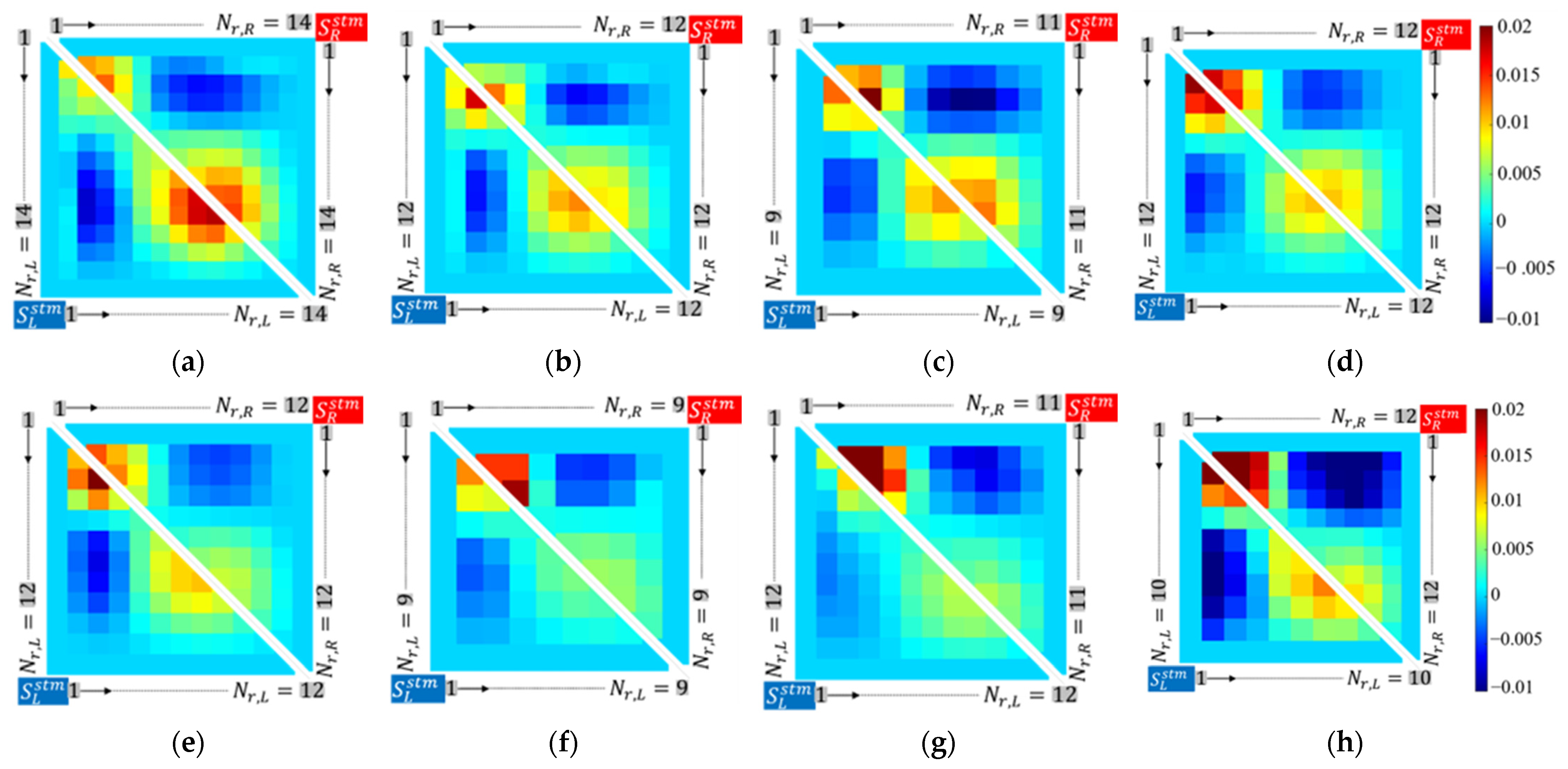
Figure 12 shows images of the rescaled step pattern covariance matrices for each foot and step frequency individually, S L stm and S R stm , previously defined in Equation (14). Note that, being symmetric, the matrices can be defined exclusively by their upper (right) or lower (left) triangular part. This allows for a compact image representation within a single figure, even though the number of points ( N r multivariate random variables) used to construct each matrix may vary due to the step pattern reduction algorithm output, outlined in Section 2.4. Consequently, the matrix dimensions correspond to those reported in Table 3, with the information retained previously being considered sufficient through the algorithm presented in Figure 6 and Figure 7.
Each pixel corresponds to a matrix element. Diagonal elements represent the N r random variable variances, while off-diagonal elements account for covariance. Red represents strong dependencies between variables that tend to increase or decrease together, notably in Figure 12d,f–h. A higher absolute value of the matrix elements reflects a greater dispersion in the stm. multivariate data, indicating increasing variability as the step frequency increases. Negative covariance accounts for variables that increase and decrease simultaneously, while null values correspond to the starting and ending points (Section 2.3.2 and Section 2.3.3). Differences between feet and across step frequencies arise, especially at 180 and 190 steps/min, highlighting the need for separate foot modelling.
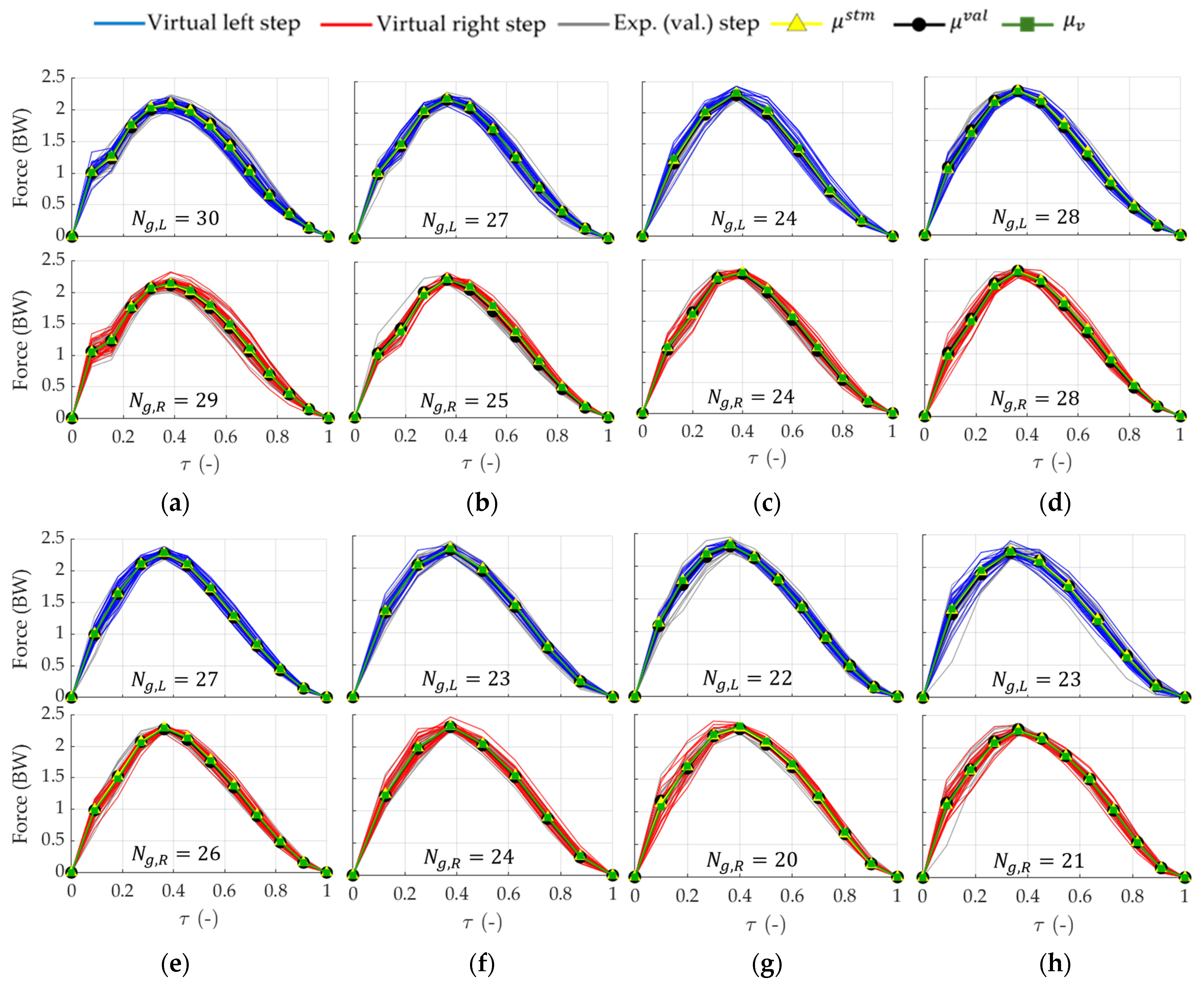
Rescaled virtual (statistically similar) steps, generated through the mvnrnd() pseudo-random number algorithm, are depicted in Figure 13. The covariance matrices in Figure 12, along with mean vectors μ stm , are fundamental for this task. As stated in Section 2.5, the remaining ( 50 % ) val. random subsets and their mean ( μ val ) are used to directly compare the shape of the virtual steps (mean μ v ). Consequently, N g , L and N g , R correspond to the sizes of the left and right val. subsets, respectively (Section 2.6). For each foot and step frequency, the step pattern reduced stochastic model satisfactorily reproduces the experimental steps. It is important to note that, when directly observing the figures of both virtual and val. subset steps, the higher covariance values—represented by the dark, mostly red, colored pixels—are directly related to the variability of the aforementioned steps, as has already been stated. For instance, the highest covariance values indicate the extent to which the first random variables (i.e., the initial interpolation points in Section 2.4, which are part of the multivariate distribution) tend to vary together. This pattern is observed in Figure 12g,h at the highest step frequencies of 190 and 200 steps/min. Therefore, a higher step dispersion in Figure 13g,h is present.
Additionally, differences between both feet at 190 steps/min remain evident and they are satisfactorily reproduced in the corresponding virtual steps at this particular step frequency. Other important features to consider, such as the dispersion among different step observations during the falling edge at 130 steps/min (Figure 12a), are also adequately replicated by the stochastic model in Figure 13a. This feature, along with the highest number of N r random variables (i.e., 14 both left-right interpolation points, Table 3) required to preserve geometric characteristics within Figure 7’s tolerances, in particular the DR (Figure 5), can explain this phenomenon.
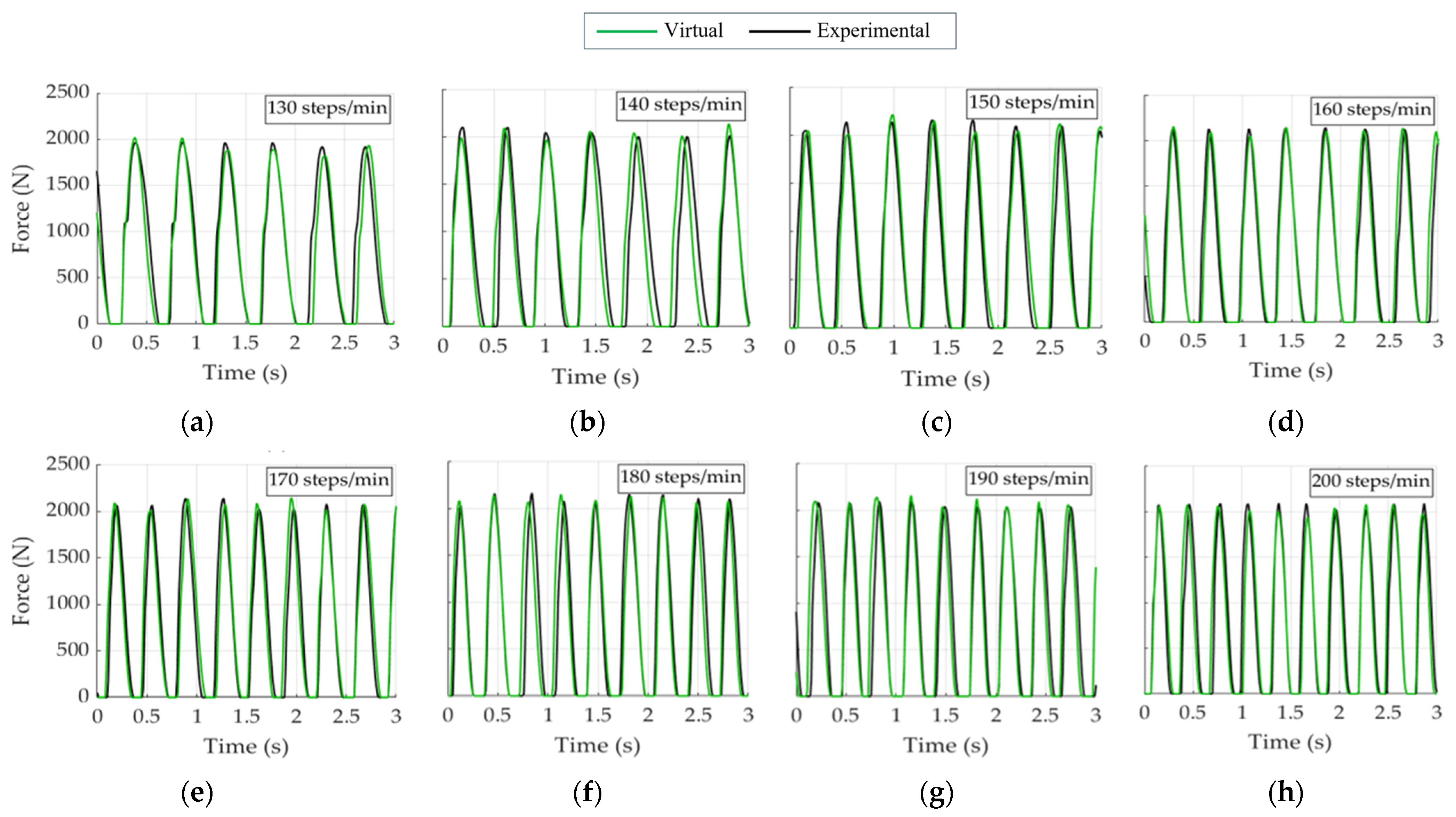
The final vertical virtual resultant GRFs are shown in Figure 14, after performing step concatenation following the guidelines in Section 2.6 and generating the corresponding virtual scaling factors and aerial times from their stm. normal distributions, ultimately concatenated according to Figure 10’s scheme. The original force scale (N) is recovered by means of the BW and the resultant action is obtained by summing the left and right forces. For representation purposes, only a 3-s relative time zoom interval is plotted for each step frequency, although the complete signals are obtained with the full sets of values. Time series from the val. random subsets (experimental data) are also plotted, obtained through concatenation in a similar way to the virtual GRFs. Note that the sampling rate has been adjusted to match the Loadsol® insoles’ f s (100 S/s), the rate at which the original data were gathered in Section 2.2. This final interpolation addresses the requirement to obtain left-right time-synchronized GRFs. Eventually, the randomness of running gait is preserved and a good match is achieved between val. and virtual data in all cases.
Time-domain virtual resultant GRF signals resemble the patterns presented in Figure 1 and Figure 3. As step frequency increases, a higher number of steps are displayed in the figures since the 3 s zoom interval remains fixed. Now, Figure 15 shows the corresponding Fourier amplitude spectra of the entire time series (not just the zoom in Figure 14), where several prominent peaks can be seen at the fundamental (metronome-driven, Section 2.2) running step frequency ( f 0 ) and its harmonics up to the 3rd one ( 2 f 0 and 3 f 0 ), given in Hz. Additionally, a quantitative comparison of the aforementioned experimental (val. data) peak values and their corresponding virtual ones is presented in terms of both frequency and amplitude in Table 8, respectively. A strong match in frequencies is observed, with errors remaining below 4.5% in all cases, the majority of them being under 2%. In contrast, larger discrepancies are found in amplitudes, with most errors below 20%, though some exceed this threshold, and the highest, mostly isolated cases, surpass 30%.

4. Discussion

Having presented the results in Section 3, a discussion is necessary to evaluate their quality, examine the strengths and limitations of the proposed stochastic model and its algorithms, and outline potential future developments to be conducted. The preservation of human gait randomness has been maintained throughout each specific task described in Section 2, keeping the intrinsic variability associated to each individual foot decoupled from that of the other foot until the final resultant GRFs, shown in Figure 14, are obtained. This is a significant advantage of the model, as the disparities between both feet are clearly evident when comparing the step pattern stm. covariance matrices in Figure 12, but are less obvious in the time series of Figure 14.
It can thus be stated that, despite ultimately assessing the resultant GRF by summing the contributions of both feet, a robust stochastic methodology is essential. All stochastic models cited in Section 1, not just the running ones but also any that entail a near-periodic action (walking, bouncing, or jumping) consider the gait cycle pattern in Figure 1 as solely the resultant GRF. On the other hand, physical models treat the GRFs as simplified deterministic actions, thereby neglecting gait variability and its real behavior.
In the context of experimental data acquisition, the Loadsol® insoles, which record running GRFs at an f s of 100 S/s, present a set of advantages and limitations, as detailed in Section 2.2. While these insoles do not offer the higher sampling rates of gold standard equipment, such as force plates and treadmills (as high as 1000 S/s), they allow for the measurement of GRFs beyond constrained laboratory settings. This feature suggests that the proposed methodology could be applied to assess human running loads in pedestrian structures such as footbridges, a specific application outlined in the Introduction (Section 1), within the field of structural engineering. Additionally, it is important to note that, despite the relatively low sampling rate, the insoles have been employed successfully at 100 S/s. Moreover, a reduction methodology has been implemented to achieve a robust description of the running GRFs while reducing the amount of data required.
The step pattern reduction algorithm presented in Section 2.4 identifies a reduced set of random variables (i.e., interpolation points) that maintain geometric characteristics within predefined tolerances (Figure 6 and Figure 7). This approach enables an efficient step pattern modelling strategy. As highlighted in Equation (15), when an excessive number of variables is used, an oversized model is obtained due to quadratic dependencies and without any advantage. To illustrate this, Table 9 shows a scenario in which the step pattern is described by 100 points for both feet, resulting in the quadratic growth in the number of parameters ( T P ) when calculating the stm. covariance matrices. In contrast, the proposed reduction strategy, with results shown in Table 3 and further discussed in Section 3, achieves reductions of more than 85% in variables and 99% in parameters.
Regarding the use of statistical tests, the HZK test has proven to be an effective tool for assessing the step pattern samples multivariate normality assumption. Out of the 16 step rescaled samples, only one fails to pass the test, belonging to the right foot at 200 steps/min (Table 4). This accounts for just 6.25% of the total samples derived from the GRF dataset (Section 2.2), and the p -value slightly leads to the null hypothesis rejection (0.0322 < 0.05). Additionally, neither the stochastic model nor the algorithms and comparisons employed were significantly affected by this deviation at the aforementioned step frequency, as seen in Table 8 when computing the errors. For these reasons, the deviation was considered bearable, and no transformation was applied to multivariate data.
On the other hand, the Box-Cox transformation enforces univariate normality across both scaling factors and aerial times, enabling the stm. random samples to meet the assumptions required for generating virtual pseudo-random values via the λ factor (Section 2.5.2). With 37.5% (12 out of 32) of the samples in Table 5 failing to pass the SW test, the need for this transformation is evident. Specifically, λ factors are computed from the MLE problem exclusively using the stm. random subsets. This preserves methodological integrity, as transforming unseen val. data and subsequently inverting the transformation compromises consistency and has no positive impact at all. At 180 and 190 steps/min, however, the transformation was completely unnecessary, as the SW test confirmed normality across all univariate samples. This coincides with the highest accuracy in estimating the first three harmonic frequencies of the virtual signal, as shown in Figure 15f,g, where relative errors between virtual and experimental Fourier spectra as low as 0.16% at 190 steps/min or even close to 0 at 180 steps/min (Table 8). Only a slight yet acceptable 2.15% deviation is observed for the 2nd harmonic at 180 steps/min. These findings confirm that, while the Box-Cox transformation enhances stochastic modelling, it can’t replace the inherent statistical nature of data.
It is also worth noting that the dataset employed, based on one pedestrian and eight step frequencies, includes fewer statistically similar steps at higher frequencies due to the constant running distance (Section 2.2). This has limited sample size (Table 1 and Table 2) for all of the random variables involved in the model. Expanding the dataset would likely enhance model robustness and is planned for future works. Furthermore, the step duration estimation (Section 2.3.2) relies on a linear extrapolation approximation (Figure 4), which can introduce slight frequency distortions. Lastly, the model step pattern is simplified using tolerances of 5% (amplitude) and 15% (location), and a 10% threshold for failed estimations, dependent on data inspection and behavior, as stated in Section 2.4.
Despite the overall performance and robustness of the proposed methodology, several limitations must be acknowledged. A higher sampling rate could be desirable for performing experimental measurements with the insoles as close as possible to the lab-constrained equipment. The reduction tolerances could also be optimized through refined criteria as previously outlined. Additionally, the dataset, while including multiple step frequencies, is currently limited to one pedestrian; thus, inter-subject variability remains unassessed. A larger dataset, as indicated in the previous paragraph, would likely enhance generalization and support deeper statistical analysis for both the same pedestrian and other groups of people. Finally, although the stochastic modelling assumptions are mostly satisfied, the minor deviation observed at 200 steps/min suggests that multivariate normal transformations to fully comply with normality may be needed in other situations.

5. Conclusions and Final Remarks

A robust algorithm has been developed for the modelling and reproduction of experimental vertical GRFs, explicitly accounting for the preservation of the inherent variability and stochastic nature of human gait during running. Consequently, a stochastic data-driven model has been formulated under normality assumptions, capable of generating sequences of virtual GRFs statistically equivalent to experimental ones. GRFs from each foot are analyzed independently, an essential procedure for identifying potential gait asymmetries and relating them to the specific characteristics of individual pedestrians. Considering that inter and intra-subject variability results in a broad spectrum of distinct GRF patterns, it becomes necessary to capture the key governing factors using a minimal set of parameters, preventing model oversizing while ensuring computational efficiency.
Accordingly, when a sufficient number of steps from a given runner is available—at any step frequency and under varying conditions—the proposed model can generate additional synthetic steps from a reduced dataset. On the other hand, the normality assumption has been examined for both the multivariate step pattern and the univariate scaling factors and aerial times employed to concatenate individual steps into virtual time series. It is important to emphasize that the stochastic data-driven model is specific to the experimental conditions under which the original data were obtained. Variations in surface, footwear, or biometric parameters may produce different model outputs. Nevertheless, the model reliably reproduces the GRFs exerted by a pedestrian under those conditions.
The results obtained and discussed in Section 3 and Section 4—particularly those related to the reproduction of harmonics in the virtual signals compared to the experimental ones—demonstrate that the model can accurately predict the time signals frequency content, provided that an adequate data processing is applied. The associated relative errors, always below 4.5% and mostly under 2%, validate the model together with step pattern reproduction in the time domain. They also indicate its potential applicability across various domains, including structural dynamics (for assessing the serviceability of pedestrian structures), as well as sports science and biomechanics. Moreover, they were achieved after reducing model complexity up to more than 50% (in terms of variables and parameters), as depicted in Section 2.4 for the step pattern.
Future work will further investigate the aforementioned potential application fields, including enhancing the model’s robustness under more challenging conditions, particularly when normality assumptions are more difficult to satisfy. In addition, since the methodology proposed in this paper is inherently adaptable to other force components and activities, the authors plan to explore the development of a unified common framework regarding different human locomotion activities. Ultimately, other research directions also aim at extending the out-of-the-lab available data, so more situations can be assessed.

Author Contributions

Conceptualization, G.F. and J.M.G.-T.; Methodology, G.F., J.M.G.-T. and A.M.; Software, G.F., Á.I.-P. and A.M.; Validation, Á.I.-P. and A.M.; Formal Analysis, G.F.; Investigation, G.F., Á.I.-P. and C.P.-R.; Resources, A.L. and A.M.; Data Curation, G.F. and C.P.-R.; Writing—Original Draft, G.F.; Writing—Review & Editing, G.F. and A.M.; Visualization, J.M.G.-T., Á.I.-P. and C.P.-R.; Supervision, J.M.G.-T., C.P.-R., A.L. and A.M.; Project Administration, A.L.; Funding Acquisition, A.L. All authors have read and agreed to the published version of the manuscript.

Funding

This research was funded by the Spanish State Research Agency (MICIU/AEI/10.13039/501100011033) and FEDER “ERDF A way of making Europe”, grant number PID2022-140117NB-I00. The research was also funded by Guillermo Fernández’s InvestigO Program grant (CP23-174)—Financed by the EU, NextGenerationEU and by the Ministerio de Universidades, Spanish Government, through the Alvaro Iglesias’ predoctoral grant number FPU21/03999.

Data Availability Statement

The original data presented in the study are openly available in [41].

Acknowledgments

During the preparation of this manuscript, the authors used ChatGPT (GPT-5) for the purposes of improving language and readability. The authors have reviewed and edited the output and take full responsibility for the content of this publication.

Conflicts of Interest

The authors declare no conflicts of interest. The funders had no role in the design of the study; in the collection, analyses, or interpretation of data; in the writing of the manuscript; or in the decision to publish the results.

Abbreviations

The following abbreviations are used in this manuscript:
GRFGround Reaction Force
BWBody weight
APActive Peak
IPImpact Peak
DRDecay Rate
GGRF area centroid
PCAPrincipal Component Analysis
PCPrincipal component
stmStochastic modelling data subset
valTesting and validation random subset
IQRInterquartile range
HZKHenze-Zirkler test
SWShapiro-Wilk test
MLEMaximum Likelihood Estimation

References

  1. Winter, D.A. Biomechanics and Motor Control of Human Movement, 4th ed.; Wiley: Hoboken, NJ, USA, 2009. [Google Scholar] [CrossRef]
  2. Nilsson, J.; Thorstensson, A. Ground reaction forces at different speeds of human walking and running. Acta Physiol. Scand. 1989, 136, 217–227. [Google Scholar] [CrossRef]
  3. Racic, V.; Pavic, A.; Brownjohn, J.M.W. Experimental identification and analytical modelling of human walking forces: Literature review. J. Sound Vib. 2009, 326, 1–49. [Google Scholar] [CrossRef]
  4. Ariki, Y.; Hyon, S.H.; Morimoto, J. Extraction of primitive representation from captured human movements and measured ground reaction force to generate physically consistent imitated behaviors. Neural Netw. 2013, 40, 32–43. [Google Scholar] [CrossRef]
  5. Bates, N.A.; Ford, K.R.; Myer, G.D.; Hewett, T.E. Impact differences in ground reaction force and center of mass between the first and second landing phases of a drop vertical jump and their implications for injury risk assessment. J. Biomech. 2013, 46, 1237–1241. [Google Scholar] [CrossRef]
  6. Lin, C.W.; Wen, T.C.; Setiawan, F. Evaluation of Vertical Ground Reaction Forces Pattern Visualization in Neurodegenerative Diseases Identification Using Deep Learning and Recurrence Plot Image Feature Extraction. Sensors 2020, 20, 3857. [Google Scholar] [CrossRef]
  7. Singh, P.; Joshi, S.D.; Patney, R.K.; Saha, K. The Fourier decomposition method for nonlinear and non-stationary time series analysis. Proc. R. Soc. A Math. Phys. Eng. Sci. 2017, 473, 2199. [Google Scholar] [CrossRef]
  8. Racic, V.; Brownjohn, J.M.W. Stochastic model of near-periodic vertical loads due to humans walking. Adv. Eng. Inform. 2011, 25, 259–275. [Google Scholar] [CrossRef]
  9. Racic, V.; Morin, J.B. Data-driven modelling of vertical dynamic excitation of bridges induced by people running. Mech. Syst. Signal Process. 2014, 43, 153–170. [Google Scholar] [CrossRef]
  10. Racic, V.; Pavic, A. Stochastic approach to modelling of near-periodic jumping loads. Mech. Syst. Signal Process. 2010, 24, 3037–3059. [Google Scholar] [CrossRef]
  11. Racic, V.; Chen, J. Data-driven generator of stochastic dynamic loading due to people bouncing. Comput. Struct. 2015, 158, 240–250. [Google Scholar] [CrossRef]
  12. Pandit, S.; Wu, S. Time Series and System Analysis with Applications, 1st ed.; Wiley: New York, NY, USA, 1990. [Google Scholar]
  13. Li, Z.; Zhang, Q.; Fan, F. A stochastic approach for generating individual jumping loads considering different jumping force patterns. J. Build. Eng. 2022, 62, 105378. [Google Scholar] [CrossRef]
  14. Chen, J.; Li, G.; Racic, V. A data-driven wavelet-based approach for generating jumping loads. Mech. Syst. Signal Process. 2018, 106, 49–61. [Google Scholar] [CrossRef]
  15. Reynolds, D. Gaussian Mixture Models. In Encyclopedia of Biometrics, 1st ed.; Springer: Boston, MA, USA, 2009; pp. 659–663. [Google Scholar] [CrossRef]
  16. Xia, F.; Liu, J.; Nie, H.; Fu, Y.; Wan, L.; Kong, X. Random Walks: A Review of Algorithms and Applications. IEEE Trans. Emerg. Top. Comput. Intell. 2020, 4, 95–107. [Google Scholar] [CrossRef]
  17. Pancaldi, F.; Bassoli, E.; Milani, M.; Vicenzi, L. A statistical approach for modeling individual vertical walking forces. Appl. Sci. 2021, 11, 10207. [Google Scholar] [CrossRef]
  18. García-Diéguez, M.; Racic, V.; Zapico-Valle, J.L. Complete statistical approach to modelling variable pedestrian forces induced on rigid surfaces. Mech. Syst. Signal Process. 2021, 159, 107800. [Google Scholar] [CrossRef]
  19. Cacho-Pérez, M.; Lorenzana, A. Walking Model to Simulate Interaction Effects between Pedestrians and Lively Structures. J. Eng. Mech. 2017, 143, 04017109. [Google Scholar] [CrossRef]
  20. Lin, B.; Zhang, Q.; Fan, F.; Shen, S. Reproducing vertical human walking loads on rigid level surfaces with a damped bipedal inverted pendulum. Structures 2021, 33, 1789–1801. [Google Scholar] [CrossRef]
  21. Liang, H.; Xie, W.; Zhang, Z.; Wei, P.; Cui, C. A Three-Dimensional Mass-Spring Walking Model Could Describe the Ground Reaction Forces. Math. Probl. Eng. 2021, 2021, 6651715. [Google Scholar] [CrossRef]
  22. Kumar, P.; Kumar, A.; Racic, V.; Erlicher, S. Modelling vertical human walking forces using self-sustained oscillator. Mech. Syst. Signal Process. 2018, 99, 345–363. [Google Scholar] [CrossRef]
  23. Xiang, Y.; Arora, J.S.; Rahmatalla, S.; Abdel-Malek, K. Optimization-based dynamic human walking prediction: One step formulation. Int. J. Numer. Methods Eng. 2009, 79, 667–695. [Google Scholar] [CrossRef]
  24. Wang, H.; Chen, J.; Brownjohn, J.M.W. Parameter identification of pedestrian’s spring-mass-damper model by ground reaction force records through a particle filter approach. J. Sound Vib. 2017, 411, 409–421. [Google Scholar] [CrossRef]
  25. Masters, S.E.; Challis, J.H. Increasing the stability of the spring loaded inverted pendulum model of running with a wobbling mass. J. Biomech. 2021, 123, 110527. [Google Scholar] [CrossRef]
  26. Zanetti, L.R.; Brennan, M.J. A new approach to modelling the ground reaction force from a runner. J. Biomech. 2021, 127, 110639. [Google Scholar] [CrossRef]
  27. Liu, D.; He, M.; Hou, M.; Ma, Y. Deep learning based ground reaction force estimation for stair walking using kinematic data. Measurement 2022, 198, 111344. [Google Scholar] [CrossRef]
  28. Peláez-Rodríguez, C.; Magdaleno, A.; Salcedo-Sanz, S.; Lorenzana, A. Human-induced force reconstruction using a non-linear electrodynamic shaker applying an iterative neural network algorithm. Bull. Pol. Acad. Sci. Tech. Sci. 2023, 71, 144615. [Google Scholar] [CrossRef]
  29. Oh, S.E.; Choi, A.; Mun, J.H. Prediction of ground reaction forces during gait based on kinematics and a neural network model. J. Biomech. 2013, 46, 2372–2380. [Google Scholar] [CrossRef]
  30. Oliveira, A.S.; Pirscoveanu, C.I.; Rasmussen, J. Predicting Vertical Ground Reaction Forces in Running from the Sound of Footsteps. Sensors 2022, 46, 9640. [Google Scholar] [CrossRef]
  31. Ancillao, A.; Tedesco, A.; Barton, J.; O’Flynn, B. Indirect Measurement of Ground Reaction Forces and Moments by Means of Wearable Inertial Sensors: A Systematic Review. Sensors 2018, 18, 2564. [Google Scholar] [CrossRef] [PubMed]
  32. Racic, V.; Pavic, A.; Brownjohn, J.M.W. Modern facilities for experimental measurement of dynamic loads induced by humans: A literature review. Shock Vib. 2013, 20, 53–67. [Google Scholar] [CrossRef]
  33. Asmussen, M.J.; Kaltenbach, C.; Hashlamoun, K.; Shen, H.; Federico, S.; Nigg, B.M. Force measurements during running on different instrumented treadmills. J. Biomech. 2019, 84, 263–268. [Google Scholar] [CrossRef] [PubMed]
  34. Magdaleno, A.; García-Terán, J.M.; Peláez-Rodríguez, C.; Fernández, G.; Lorenzana, A. Generating vertical ground reaction forces using a stochastic data-driven model for pedestrian walking. J. Comput. Sci. 2025, 88, 102602. [Google Scholar] [CrossRef]
  35. García-Terán, J.M.; Magdaleno, A.; Fernández, J.; Lorenzana, A. A statistical-based procedure for generating equivalent vertical ground reaction force-time histories. In Proceedings of the 5th International Conference on Mechanical Models in Structural Engineering (CMMoST), Alicante, Spain, 23 November 2019. [Google Scholar]
  36. Tahir, A.M.; Chowdhury, M.E.; Khandakar, A.; Al-Hamouz, S.; Abdalla, M.; Awadallah, S.; Reaz, M.B.; Al-Emadi, N. A Systematic Approach to the Design and Characterization of a Smart Insole for Detecting Vertical Ground Reaction Force (vGRF) in Gait Analysis. Sensors 2020, 20, 957. [Google Scholar] [CrossRef]
  37. Weidensager, L.; Krumm, D.; Potts, D.; Odenwald, S. Estimating vertical ground reaction forces from plantar pressure using interpretable high-dimensional approximation. Sports Eng. 2024, 27, 3. [Google Scholar] [CrossRef]
  38. Seiberl, W.; Jensen, E.; Merker, M.; Leitel, M.; Schwirtz, A. Accuracy and precision of loadsol® insole force-sensors for the quantification of ground reaction force-based biomechanical running parameters. Eur. J. Sport Sci. 2018, 18, 1100–1109. [Google Scholar] [CrossRef]
  39. Renner, K.E.; Blaise Williams, D.S.; Queen, R.M. The reliability and validity of the Loadsol® under various walking and running conditions. Sensors 2019, 19, 265. [Google Scholar] [CrossRef]
  40. Burns, G.T.; Deneweth Zendler, J.; Zernicke, R.F. Validation of a wireless shoe insole for ground reaction force measurement. J. Sports Sci. 2019, 37, 1129–1138. [Google Scholar] [CrossRef]
  41. Fernández, G.; García-Terán, J.M.; Lorenzana, A.; Magdaleno, A. A reduced stochastic data-driven approach to modelling and generating vertical ground reaction forces during running. Mendeley Data 2025. [Google Scholar] [CrossRef]
  42. Henze, N.; Zirkler, B. A class of invariant consistent tests for multivariate normality. Commun. Stat. Theory Methods 1990, 19, 3595–3617. [Google Scholar] [CrossRef]
  43. Henze-Zirkler’s Multivariate Normality Test. Available online: https://tinyurl.com/dxd9edh3 (accessed on 9 March 2025).
  44. Greenacre, M.; Groenen, P.J.F.; Hastie, T.; D’Enza, A.I.; Markos, A.; Tuzhilina, E. Principal component analysis. Nat. Rev. Methods Primers 2022, 2, 100. [Google Scholar] [CrossRef]
  45. Shapiro, S.S.; Wilk, M.B. An analysis of variance test for normality (complete samples). Biometrika 1965, 52, 591–611. [Google Scholar] [CrossRef]
  46. Shapiro-Wilk and Shapiro-Francia Normality Tests. Available online: https://tinyurl.com/3secru59 (accessed on 9 March 2025).
  47. Box, G.E.P.; Cox, D.R. An Analysis of Transformations. J. R. Stat. Soc. Ser. B Stat. Methodol. 1964, 26, 211–243. [Google Scholar] [CrossRef]
  48. Pan, J.X.; Fang, K.T. Maximum Likelihood Estimation. In Growth Curve Models and Statistical Diagnostics, 1st ed.; Springer: New York, NY, USA, 2002; pp. 77–158. [Google Scholar] [CrossRef]
  49. Scott, D.W. Sturges’ rule. WIREs Comput. Stat. 2009, 1, 303–306. [Google Scholar] [CrossRef]
  50. MATLAB Statistics and Machine Learning Toolbox: Function mvnrnd(). Available online: https://www.mathworks.com/help/stats/mvnrnd.html (accessed on 9 March 2025).
  51. Tong, Y.L. Fundamental Properties and Sampling Distributions of the Multivariate Normal Distribution. In The Multivariate Normal Distribution, 1st ed.; Springer: New York, NY, USA, 1990; pp. 23–61. [Google Scholar] [CrossRef]
  52. Mecklin, C.J.; Mundfrom, D.J. A Monte Carlo comparison of the Type I and Type II error rates of tests of multivariate normality. J. Stat. Comput. Simul. 2005, 75, 93–107. [Google Scholar] [CrossRef]
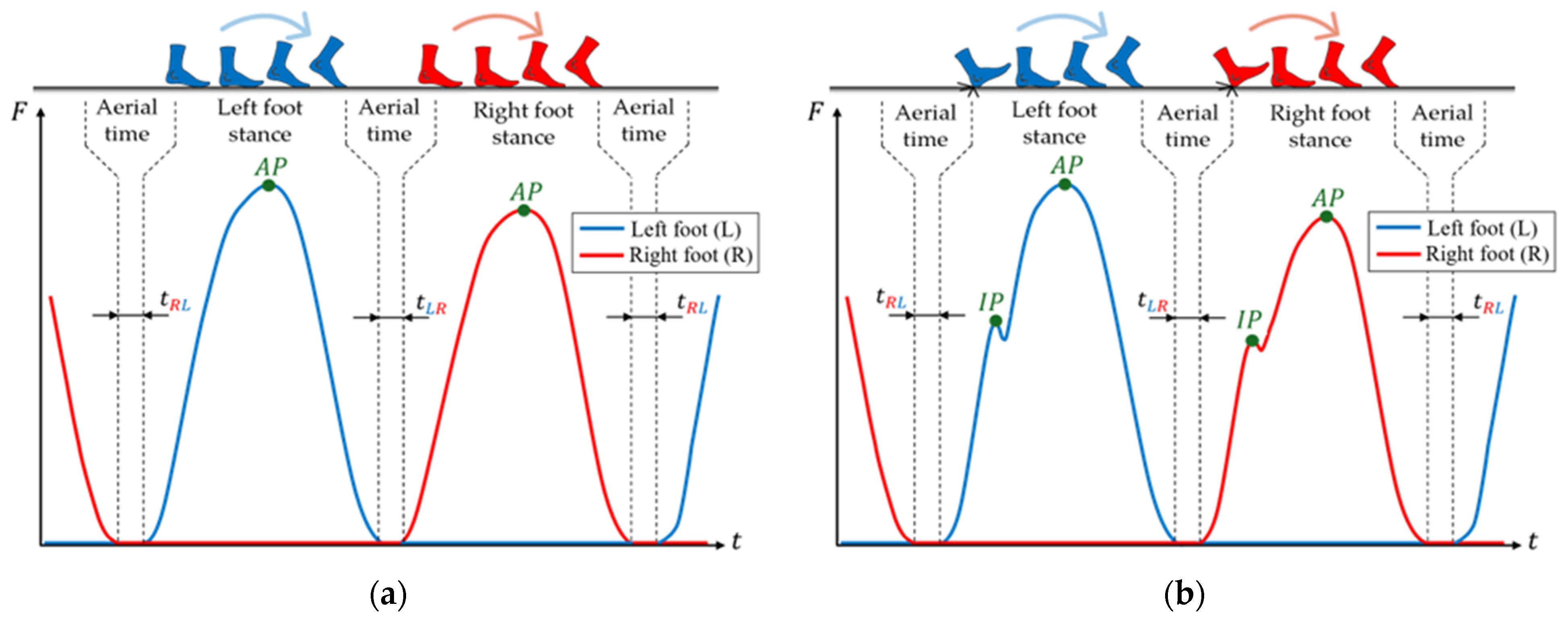
Figure 1. Vertical running GRFs patterns. Left (blue) and right foot (red) forces with the four phases of the gait cycle: (a) mid-frontfoot runners; (b) rearfoot (heel strike runners).
Modelling 06 00144 g001
Figure 2. Instrumented insoles: (a) Novel GmbH Loadsol® model; (b) Usage example.
Modelling 06 00144 g002
Figure 3. Example of measured time-synchronized GRF signals at 130 steps/min.
Modelling 06 00144 g003
Figure 4. Step detection, time isolation and duration estimation by means of linear extrapolation.
Modelling 06 00144 g004
Figure 5. Rescaled step geometric variables scheme: AP, DR and G.
Modelling 06 00144 g005
Figure 6. Flowchart of the rescaled step pattern reduction algorithm: main, successive interpolation (red dashed), and nested geometric variable evaluation loop (blue dashed).
Modelling 06 00144 g006
Figure 7. Detail of the nested loop in the rescaled pattern reduction algorithm (Figure 6): geometric variable estimations and e count calculation procedure.
Modelling 06 00144 g007
Figure 8. Histograms and normal distributions for scaling factors and aerial times, with Box-Cox transformation applied when necessary (140 steps/min): (a) Transformed left steps scaling factor ( η L stm ); (b) η R ; (c) t L R ; (d) Transformed RL aerial time ( t R L stm ).
Modelling 06 00144 g008
Figure 9. Example of a virtual rescaled step generated by means of MATLAB®’s mvnrnd(), compared to an N univariate normal distribution approach (130 steps/min).
Modelling 06 00144 g009
Figure 10. Example of virtual step concatenation (100 S/s, 130 steps/min), with the order in which operations are sorted (pink) in the final, time-synchronized GRF signals.
Modelling 06 00144 g010
Figure 11. Full Materials & Methods summary, with references to sections for a broader description.
Modelling 06 00144 g011
Figure 12. Covariance matrix images for each rescaled foot step pattern ( 50 % stm. random subsets): left steps ( N r , L × N r , L ) matrix S L stm (lower triangular), and right steps ( N r , R × N r , R ) matrix S R stm (upper triangular): (a) 130; (b) 140; (c) 150; (d) 160; (e) 170; (f) 180; (g) 190; (h) 200 steps/min.
Modelling 06 00144 g012
Figure 13. Graphical rescaled pattern comparison among virtual (blue-left, red-right) and experimental val. random subset steps (grey) for each step frequency, with stm. (yellow), val. (black) and virtual (green) mean vectors also represented: (a) 130; (b) 140; (c) 150; (d) 160; (e) 170; (f) 180; (g) 190; (h) 200 steps/min.
Modelling 06 00144 g013
Figure 14. Time comparison between the experimental (val. data, black) and virtual (green) vertical resultant GRFs (100 S/s): (a) 130; (b) 140; (c) 150; (d) 160; (e) 170; (f) 180; (g) 190; (h) 200 steps/min.
Modelling 06 00144 g014
Figure 15. Fourier amplitude spectra of both the experimental (val. data, black) and virtual (green) GRFs in Figure 14. Val. data (red) and virtual (magenta) peaks corresponding to the first three harmonics are also highlighted: (a) 130; (b) 140; (c) 150; (d) 160; (e) 170; (f) 180; (g) 190; (h) 200 steps/min.
Modelling 06 00144 g015
Table 1. Step sample sizes after detection and outlier removal stages, shown as left-right (L-R).
Step Frequency
(Steps/min)
m 0 —Detection m 1 —Duration m —Pattern
LRLRLR
130666663626158
140636360545451
150606057544949
160636359595756
170606156575453
180535349504649
190515147474441
200535347484642
Table 2. Aerial time sample sizes after outlier removal stage.
Step Frequency (Steps/min) t L R t R L
m 0 , L R m 1 , L R m 0 , R L m 1 , R L
13064616461
14060596160
15058575757
16061606260
17057575756
18051515151
19049474947
20049475049
Table 3. Step pattern reduction algorithm N r values (interpolation points) and reduction coefficients K .
Step Frequency
(Steps/min)
Left Steps PointsRight Steps Points
N 1 N r K (%) N 1 N r K (%)
130341458.8351460.0
140311261.3341264.7
15029969.0301163.3
160271255.6291258.6
170271255.6271255.6
18024962.524962.5
190231247.8231152.2
200231056.5221245.5
Table 4. HZK multivariate normality test p-values and d PCs for step pattern samples after PCA.
Step Frequency
(Steps/min)
Left StepsRight Steps
p-valuedLp-valuedR
1300.36630.1613
1400.23430.3703
1500.70330.07823
1600.55330.4843
1700.59740.3883
1800.11330.5443
1900.78440.4083
2000.36330.03223
Table 5. SW univariate normality test results for scaling factors and aerial times, with Box-Cox transformation ( λ factor and new p -value over 50 % stm. random subset, p λ stm ) applied if the sample data failed to pass the test.
Step Frequency
(Steps/min)
Scaling FactorsAerial Times
η L η R t L R t R L
p -value λ p λ stm p -value λ p λ stm p -value λ p λ stm p -value λ p λ stm
1300.0172−7.320.2410.0547--0.237--0.0683--
1400.00396−7.700.9270.265--0.0799--0.0101−1.640.487
1500.252--0.0694--0.03220.3940.6700.117--
1600.0268−2.720.1530.144--0.04200.5130.1960.03000.8020.179
1700.0428−8.320.2050.0221−4.380.3320.148--0.00533−0.4810.483
1800.334--0.0501--0.148--0.174--
1900.152--0.143--0.245--0.189--
2000.728--0.03742.070.1050.581--0.002643.440.0803
Table 6. Scaling factors normal distribution parameters for the stm. random subsets ( 50 % of each sample).
Step Frequency
(Steps/min)
η L stm η R stm
μ stm σ stm μ λ stm σ λ stm 1 0 5 μ stm σ stm μ λ stm σ λ stm
130--0.1373.142.630.137--
140--0.1301.062.860.104--
1503.270.190--3.160.133--
160--0.3551573.340.147--
170--0.1200.106--0.227 1.90 10 4
1803.960.181--3.890.268--
1904.180.269--4.140.246--
2004.440.197----9.611.26
Table 7. Aerial times normal distribution parameters for the stm. random subsets ( 50 % of each sample).
Step Frequency
(Steps/min)
t L R stm t R L stm
μ stm σ stm μ λ stm σ λ stm μ stm σ stm μ λ stm σ λ stm
1300.08530.0225--0.08880.0189--
1400.08340.0236----−36.010.4
150--−1.550.08950.08970.0149--
160--−1.460.0537--−1.060.0191
1700.07600.0149----−5.200.560
1800.07510.0139--0.07470.0188--
1900.06460.0206--0.09640.0122--
2000.06370.0131----−0.291 1.81 10 5
Table 8. Peak frequencies corresponding to the first three harmonics in the Fourier plots of Figure 15 for both experimental (val. data) and virtual resultant GRFs.
Step FrequencyExperimental (Test) (Hz)Virtual (Hz)Error (%)
Steps/minHz f 0 2 f 0 3 f 0 f 0 2 f 0 3 f 0 E f 0 E 2 f 0 E 3 f 0
1302.172.184.366.542.134.276.592.132.130.678
1402.332.314.636.942.314.626.650.2310.234.22
1502.502.464.927.482.514.927.442.200.07090.600
1602.672.675.347.922.675.287.950.2381.130.363
1702.832.855.758.592.795.538.321.933.803.18
1803.003.006.069.063.005.939.06<0.012.15<0.01
1903.173.196.389.573.186.379.550.1590.1590.159
2003.333.346.769.553.356.709.810.2390.9402.745
Table 9. Model’s final total variables ( T V ) and parameters ( T P ) given by Equation (15), compared to the situation in which 100 points had been used to model each foot’s step pattern.
Step Frequency (Steps/min) T V T V , 100 T V T V , 100 % T P T P , 100 T P T P , 100 %
1303284.321997.8
1402886.316598.4
1502488.212098.8
1602886.316598.4
1702886.316598.4
1802289.29999.0
1902786.815398.5
2002687.314298.6
Disclaimer/Publisher’s Note: The statements, opinions and data contained in all publications are solely those of the individual author(s) and contributor(s) and not of MDPI and/or the editor(s). MDPI and/or the editor(s) disclaim responsibility for any injury to people or property resulting from any ideas, methods, instructions or products referred to in the content.