Abstract
Traditional median filtering with a fixed window easily leads to edge blurring and adaptive median filtering requires manual presetting of the maximum window parameter and has insufficient retention of details when dealing with high-density salt-and-pepper noise. Aiming at these problems, this paper proposes a hybrid decision-making adaptive median filtering algorithm with dual-window detection in collaboration with particle swarm optimization (PSO). The algorithm quickly locates suspected noise points through a 3 × 3 small window and enhances noise identification accuracy by using a PSO dynamically optimized 5–35-pixel large window. Meanwhile, a hybrid decision-making mechanism based on local statistical properties was introduced to dynamically select median filtering, weighted average based on spatial distance, or pixel preservation strategy to balance noise suppression and detail preservation, and the PSO algorithm was used to automatically find the optimal parameters of the large window’s size to avoid the manual parameter-tuning process. Experiments were conducted on standard grayscale and color images and compared with four traditional methods and two more advanced methods. The experiments showed that the algorithm improved the peak signal-to-noise ratio (PSNR) value by 2–4 dB and the structural similarity index measure (SSIM) metric by 0.05–0.2 under high salt-and-pepper noise density compared with the traditional methods, which effectively improved the contradiction between noise suppression and detail retention in traditional filtering algorithms and provided a highly efficient and intelligent solution for image denoising in high-noise scenarios.
1. Introduction
During image acquisition, transmission, and storage, noise is difficult to avoid due to defective imaging equipment, complex environments, and impulse signal interference. Salt-and-pepper noise (SPN) [1] is the most common and harmful type of noise, which was named because of its black and white spots on an image. This type of noise can cause sensor unit failure and pixel conversion errors, which not only significantly reduce the visual quality of images, but also seriously interfere with subsequent processing tasks such as image segmentation and feature extraction. Therefore, exploring efficient and accurate SPN removal methods has always been a key research direction in the fields of computer vision and image processing [2].
In the early exploration of denoising techniques, nonlinear filters occupied an important position in the field of denoising by virtue of their high adaptability to the impacts of characteristics of SPN [3,4,5]. Among them, the classical median filter (MF) [6,7] achieved denoising by replacing the value of the center pixel with the median value of the pixels in the filter window, which can suppress SPN; however, this uniform treatment often blurred the details and edges of an image, resulting in the loss of structural information. Mean value filtering (MF) [8,9] replaced noise points with the mean value of neighboring pixels, which can smooth an image but also caused the same problem of blurring the edges, making it difficult to meet application scenarios with high requirements for image details.
In order to overcome the limitations of traditional methods, many scholars have carried out a large number of studies on improving median filtering and mean filtering. For the optimization of the median filter, a series of improved algorithms have emerged one after another. The weighted median filter (WMF) [10] retained image details more flexibly in the noise removal process by assigning weights to pixels at different positions. The adaptive fuzzy switching median filter (AFSM) adopted a fuzzy logic system [11] to intelligently select a filtering strategy according to the local features of an image, which improved the adaptive capability of denoising. The adaptive median filter (AMF) [12] was more innovative in proposing the idea of dynamically adjusting the filter window size according to the noise density. A large window was used to recognize and eliminate noise more accurately in the face of strong noise pollution. A small window was used in less noisy regions to protect image details. In addition, Riji et al. [13] proposed a direction-weighted fuzzy median filtering noise detection and noise reduction method to improve the poor denoising capabilities of traditional methods in high-density noise scenes. By introducing a fuzzy gradient value to accurately detect noise and using the direction-weighted median of neighboring pixels for filtering processing, the filtering effect and image quality were significantly improved. Wang et al. [14] proposed an improved adaptive median filtering method. The method adaptively increased the window’s size and subdivided the window into smaller parts. Then, multiple median calculations were performed on the segmented window to ensure the validity of the median. Many important results have also been achieved in research on improving mean value filtering. The adaptive iterative mean filtering (AIMF) algorithm proposed by Guo et al. [15] has surpassed the limitations of traditional single filtering. Multiple rounds of iterative denoising were applied to noise points to gradually optimize the pixel values. In contrast to traditional filtering algorithms, it showed obvious advantages in removing high-density noise. Zhang et al. [16] proposed an adaptive nonlocal mean filter for removing SPN. The algorithm combined the characteristics of the SPN and the nonlocal similarity of an image and reconstructed the information by adaptively detecting noise points and adopting a specific filtering window. While removing SPN, the structural information of the image was better preserved, and the denoising performance of the image was improved. Li et al. [17] proposed a new filtering algorithm with dynamic adjustment of weighting coefficients. The algorithm used dynamic weighting coefficients to balance the filtering process of fast median filtering and mean filtering so that they can reflect their respective advantages, make up for each other’s deficiencies, and achieve good denoising results.
With the continuous advancement of research, both deep learning technology and the particle swarm optimization (PSO) algorithm for parameter optimization have demonstrated unique advantages in the field of image restoration. Fu et al. [18] proposed the nonlocal switching filtered convolutional neural network (NLSF-CNN) and constructed the denoising model by using NLSF preprocessing and CNN training. Putra et al. [19] utilized the convolutional visual transformer (CvT) with Residual Network (ResNet) architecture to design RTF-Net. Rafiee et al. [20] proposed a deep CNN model (SeConvNet). In this model, a new selective convolution (SeConv) block was introduced to suppress salt-and-pepper noise in grayscale and color images. A very significant denoising effect was achieved. Siddique et al. [21] proposed a novel deep learning framework that combines 1D conv ResNet, MHSA, and BiLSTM. This hybrid method enhances feature extraction, suppresses noise, and captures remote dependencies in non-stationary and nonlinear signals. Zhou et al. [22] introduced an adaptive contraction and expansion factor based on the cooperative quantum particle swarm optimization (CQPSO) algorithm. The improved cooperative quantum particle swarm optimization (QPSO) algorithm was used to optimize the regulation factor and threshold in the wavelet threshold function. It significantly improved the image denoising effect. Hassan et al. [23] proposed a threshold selection method by integrating particle swarm optimization and late acceptance hill-climbing heuristic algorithms. This method outperformed other methods in terms of the signal-to-noise ratio and root mean square error of the noise-removed transmitted signal. Although these methods significantly improved the denoising performance, most of them came at the cost of increasing algorithm complexity and computational resource consumption. Therefore, reducing time and space complexity while guaranteeing an excellent denoising effect and realizing efficient and fast pepper noise removal is still a core problem that needs to be solved in academia and industry at present and points out an important direction for subsequent research.
This paper proposes a hybrid decision-making adaptive median filtering algorithm with dual-window detection and particle swarm optimization (PSO). The algorithm adopts a dynamic window detection mechanism and particle swarm optimization algorithm to achieve intelligent parameter adjustment, aiming at effectively suppressing SPN while retaining image details and edge information to the maximum extent and providing a new technical solution for the field of image denoising. The main innovations are as follows:
- (1)
- Aiming at the defects of the traditional fixed window for noise detection, a dual-window cooperative detection and dynamic adaptation strategy was proposed. A 3 × 3 small window was used to quickly screen noise, combined with a 5 × 5–35 × 35 dynamic large window to adaptively expand the detection range, enhance noise recognition accuracy in complex scenes, and balance detection efficiency and accuracy by cascading the large and small windows.
- (2)
- The particle swarm optimization algorithm was applied to address the problem of traditional filtering requiring manual parameter adjustment and having poor generalization. Taking PSNR as the target, the optimal parameters of 5 × 5–35 × 35 windows were searched automatically to realize the adaptive adjustment of different noise densities, which solved the limitation of traditional filtering relying on manual parameter adjustment.
- (3)
- Aiming at the problem that traditional filtering often blurs image edges, this study proposed a weighted averaging mechanism based on spatial distance. The weight model was constructed based on the Gaussian kernel; weights were assigned according to the inter-pixel distance, and high weights were given to near distances, which effectively preserved the image edges and texture details when removing pepper noise.
- (4)
- Aiming at the problem of a single traditional filtering strategy, this paper proposed a hybrid decision-making strategy. By analyzing the pixel characteristics of the double window and judging the degree of noise and texture complexity, the median filtering, weighted average, or original value retention strategy was adaptively selected to achieve accurate denoising and efficiency optimization in different scenarios.
2. Basic Principles
2.1. Adaptive Median Filtering (AMF)
SPN in an image appears randomly in the form of high amplitude (salt noise) or low amplitude (pepper noise) noise, and the pixel value of a noise point usually deviates significantly from its neighboring grayscale value. Classical nonlinear filtering uses SPN’s characteristic of being impactful to perform noise elimination through the detection and substitution of abnormal pixel values. Adaptive median filtering achieves noise elimination by detecting and substituting noise points in square windows of different sizes.
Assuming that is a square image region centered at and with side length in a contaminated image, is the pixel value at the center position , and and are the minimum, median, and maximum values of the image block, respectively. For the center pixel of the image block, the output value of the adaptive median filter can be obtained by the following Algorithm 1:
| Algorithm 1 Adaptive Median Filtering |
| 1: . |
| 2: of the image block. |
| 3: then |
| 4: go to step 11. |
| 5: |
| 6: end if |
| 7: then |
| 8: go to step 2. |
| 9: |
| 10: end if |
| 11: then |
| 12: |
| 13: |
| 14: end if |
AMF achieved better performance in removing SPN by two steps of noise finding and replacement of noise pixel values, but it still had shortcomings: (1) Its way of judging whether a pixel was a noise point was only based on whether the pixel was an extreme point in a fixed window. It was not precise enough and was prone to misjudgment. Especially when the image pixel value was close to the maximum or minimum value, the real value may have been eliminated as noise. (2) The maximum window size needed to be manually pre-set and lacked the adaptive ability to match the noise density and texture complexity of different images, which may have resulted in a situation where the window was not large enough to contain enough non-noise pixels under high noise density or where the edges of the complex texture region were damaged due to the oversized window. (3) It was ineffective in dealing with high-density noise. When the noise density was high, most of the windows were noise points, and even if the window was expanded to the maximum window size, the median value might still have been a noise value, which led to a failure in denoising.
2.2. Particle Swarm Optimization Algorithm (PSO)
PSO is a population smart optimization algorithm inspired by the foraging behavior of bird flocks [24,25,26]. The optimal solution is found by modeling the collaboration and competition of particles in the search space. The core idea was to use the historical experience of individuals and the experience of other individuals in the group to adjust their behaviors, so as to achieve the solutions of complex optimization problems. In PSO, a population of m particles can be represented as . When it is in an n-dimensional space, the position where the particle is located is represented by .
Each position represents a candidate solution to the optimization problem. A particle searches for a better solution by iteratively updating its position. The best position searched by the ith particle is called the individual optimal solution, denoted as . The best position experienced by the whole swarm of particles, i.e., the currently searched optimal solution, is called the global optimal solution, denoted as Each particle has a velocity, denoted as , and when both optimal solutions are found, each particle updates its velocity and position according to Equations (1) and (2).
Velocity vector iteration equation:
Position vector iteration equation:
where represents the velocity of the ith particle in the d-dimension after the (k + 1)th iteration and is the inertia weight. By adjusting the size of , the global optimization ability and the local optimization ability can be adjusted. are the learning factors, which control the degree of convergence of the particles to the individual optimal and global optimal positions, respectively. are random numbers between 0–1. denotes the individual optimal solution in the d-dimensional space after the kth iteration. denotes the global optimal solution in the d-dimensional space after the kth iteration.
3. Method
To solve the noise detection one-sidedness, the limitations of manually setting window parameters, and the failure risk in high-density noise scenes faced by the AMF algorithm in removing SPN, this paper proposed a hybrid decision-making adaptive median filtering algorithm with dual-window detection and synergistic particle swarm optimization. This method significantly improves the adaptability and denoising accuracy of the algorithm in complex noise environments through a layered noise detection mechanism, PSO dynamic parameter optimization, and a hybrid filtering strategy.
3.1. Dual-Window Layered Noise Detection Model
(1) Small window primary detection
In this paper, images were scanned pixel-by-pixel through a small window to conduct the primary detection of SPN. For the center pixel of the window, the minimum value and the maximum value of pixels in the window were calculated, and the primary judgment of noise was performed based on the extreme value range, as shown in Equation (3).
indicates the state of the pixel point, , which represents that the pixel point is suspected to be noisy, and , which indicates that it is not noisy. This step quickly found the potential location of the SPN pixels by local extreme value comparison in a small window, providing a candidate set for subsequent fine verification. It also avoided over-processing of normal pixels and improved the detection efficiency.
(2) Large window secondary verification
After initial screening of suspected noise points by primary detection (), the algorithm extended the window to a dynamic large window. The size was determined by PSO. These suspected noise points were confirmed with more precise structural features.
In the large window verification stage, the center pixel was judged again by calculating the new minimum value and maximum value in the window, as shown in Equation (4).
If was still equal to or equal to , the pixel was finally judged as a noise point, i.e., ; otherwise, it was recognized as a real extreme point of the image and was retained.
This dual-window cascade detection mechanism improved the accuracy of noise detection. With wider pixel sampling and more comprehensive structural characterization, the large window effectively reduced misjudgments caused by local extreme value fluctuations. Especially when dealing with images with large areas of single tones or complex textures, it was able to more accurately distinguish between noise and real pixels, thus significantly improving the reliability of noise detection.
3.2. Hybrid Filtering Decision Model
The proposed hybrid filtering model, based on the median extreme value characteristics in small windows and the distribution of non-noise pixels, achieved adaptive processing for scenarios with different noise densities. The specific logical implementation of this model was as follows.
When double-window detection determined that the center pixel was a noise point (), the median value of the small window (3 × 3) was first calculated, and the noise density was determined by whether was the extreme value of the small window, i.e., or .
(1) Low-density noise (noise density 50%)
If was not the extreme value of the small window, it indicated that non-noise pixels were in the majority within the small window. In this case, the model directly used the small window median filtering to repair the noise points. The median could effectively represent the true pixel value, suppressing noise while avoiding excessive smoothing.
(2) High-density noise scene (50% noise density 90%)
If was the extreme value of the small window, it indicated that the proportion of noise within the small window was high. In this case, the model selected non-noise pixels within the large window (with the size optimized by PSO) for further repair. The specific steps were as follows: First, extract the non-noise pixels in the large window (). Then assign Gaussian weights to the non-noise pixels according to their Euclidean distance from the center of the window and compute the weighted mean value for repair, as shown in Equations (5) and (6):
where represents the pixel value of the central pixel after denoising, represents the large window region, represents the weight, represents the pixel value of , and is the Euclidean distance from pixel to the center of the window, with the nearest neighboring pixels having a higher weight. This strategy reduced the effect of noise by weighted averaging while preserving edge structure.
(3) Extremely dense noise scenes (noise density > 90%)
If there was no non-noise pixel within the large window, the model used the median filtering of the large window for forced repair. Although the median may still have contained noise at this point, the risk of noise dominance was reduced by expanding the window to include as many potentially real pixels as possible.
For non-noise points determined by double-window detection, the original value was directly retained to ensure that the image details were not disturbed.
3.3. PSO Dynamic Parameter Optimization Model
3.3.1. Optimization Objective
The large window’s size was defined as the optimization variable, whose value directly affected the spatial extent of noise detection and the ability to retain image details. Considering that the range of the filter window should be odd to ensure center symmetry, the search range of the large window was set to be an odd number in the interval [5, 35]. The PSNR of the denoised image was used as the objective function [27], as shown in Equation (7).
where is the original image and is the denoised image.
3.3.2. PSO Design and Implementation
The position of each particle represented a candidate window size, and the velocity of a particle indicated how the particle moved from its current position (current window size) to a new position (better window size). The specific process of PSO co-optimizing the maximum window size was as follows:
(1) Initializing the positions and velocities of each particle.
The initial position of each particle was a randomly generated odd number within the range of [5, 35]. The initial velocity of each particle was constrained within the interval of [−2, 2] to prevent particles from escaping the search space. A swarm size of 10 particles was used to balance computational efficiency and search accuracy.
(2) Initializing the individual best solutions, i.e., , and the global best solution, i.e., , of the initial particles.
The initial individual was the initial position of each particle. Based on the initial position of each particle, different denoised images were obtained using the algorithm proposed in this paper. Then the objective function values of these different denoised images were calculated using Equation (5). The position of the particle that maximizes the objective function value is the initial global best solution .
(3) Updating the velocity and position of each particle.
The velocity and position of each particle was updated using Equations (1) and (2). The inertia weight was set to 1.1, the individual learning factor , and social learning factor .
(4) Updating and .
Based on the current position of each particle, the objective function value of the new denoised image was recalculated. If this value was greater than the previous one, the was updated to the current position of the particle. Similarly, the was updated.
(5) The algorithm checked whether the maximum number of iterations had been reached. If not, it returned to step (3) and continued iterative updates; otherwise, it proceeded to step (6).
(6) The algorithm used the final (optimal maximum window size) to perform the final denoising output and obtain the optimal denoised image.
The overall flow of the algorithm in this paper is shown in Figure 1.
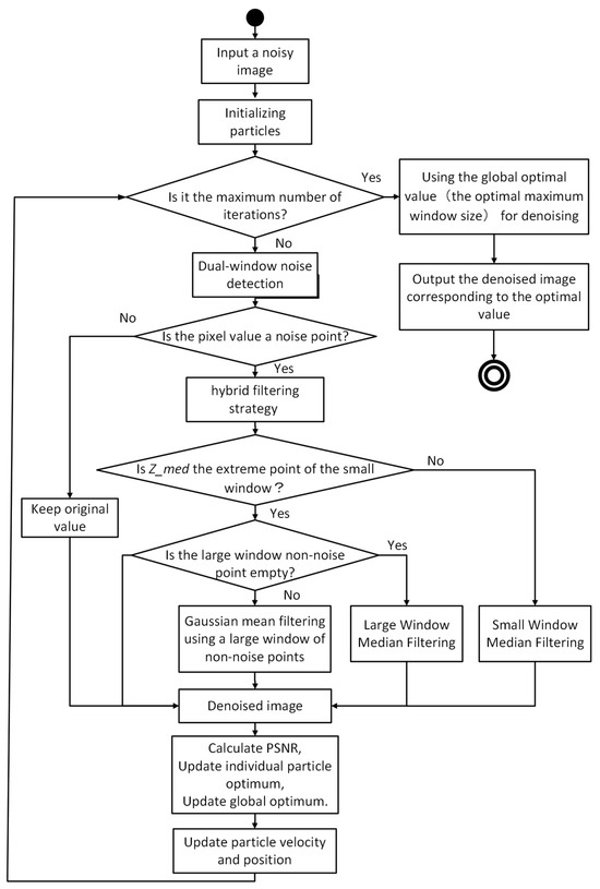
Figure 1.
The overall flow of the algorithm.
4. Experimental Results and Analyses
4.1. Image Quality Evaluation Methods
To evaluate the quality of the denoised images, the peak signal-to-noise ratio (PSNR) and structural similarity (SSIM) were used as evaluation criteria, as shown in Equations (7) and (8).
where , , , and are the mean intensity, standard deviation, and cross-covariance of the images and , respectively. and are the two constants used to keep the equations stable.
4.2. Test Results
4.2.1. Grayscale Image Test
The equipment configuration for this experiment was Intel(R) Core(TM) I5-7500, 8.00 GB of RAM, Windows 10 system, and the processing software was MATLAB R2023b. Twelve grayscale images from the standard test dataset Set12 were selected as experimental objects, and denoising tests were carried out by adding different densities of SPN.
Table 1 shows the average PSNR results after denoising 12 images by different denoising methods. When the noise density was 70%, the average PSNR value of this paper’s algorithm was improved by 2.38 dB compared with the classical AMF, 1.8 dB compared with the AWMF [28], 1.65 dB compared with the literature [16], and 1.21 dB compared with the literature [17], which fully verified its effectiveness and balance between noise removal and image fidelity. The data indicated that, among all the compared methods, the performance of this paper’s method was better, and higher PSNR values were obtained, which verified its validity and advancement.

Table 1.
Comparison of average PSNR across different denoising methods.
For the same set of images, Table 2 presents the SSIM results obtained by applying different denoising methods. Among many denoising methods, the SSIM values of this paper’s method are still the highest. A high SSIM value implies that the denoised image is highly compatible with the original image at the structural level and retains the key features of the image. The texture, edges, and other key features of the image remain intact. The method in this paper was able to obtain a higher average SSIM value under the interference of high-density SPN, which fully demonstrates its excellent ability to maintain the structural integrity of an image.
Table 2.
Comparison of average SSIM across different denoising methods.
Figure 2 and Figure 3 show the average PSNR and average SSIM attained by this paper’s method against six comparable methods in the Set12 dataset. The experimental results indicate that, in contrast to the AMF and AWMF methods, the average PSNR and SSIM of this method achieved a significant increase, which fully verified the optimization effect of the dual-window detection mechanism and the hybrid filtering strategy on denoising performance. Meanwhile, the introduction of the PSO algorithm provided the ability to conduct adaptive parameter adjustment, which further enhanced the effectiveness of the method. On the other hand, when dealing with high-density noise, the PSNR and SSIM of this paper’s method still maintained a high growth trend compared with the literature [16] and the literature [17], which fully proves the significant advantage of this paper’s method in removing high-density noise.
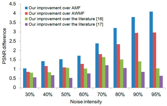
Figure 2.
The trend of PSNR growth of this method versus other methods.
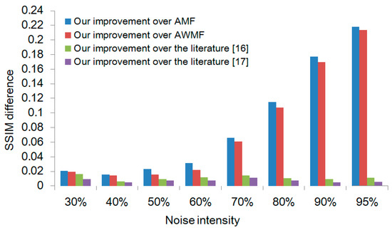
Figure 3.
The trend of SSIM growth of this method versus other methods.
Three typical images were randomly selected from Set12 for denoising experiments, and the results are presented in Table 3 and Table 4. The experimental data shows that this paper’s method significantly surpassed the other algorithms in PSNR and SSIM. Taking the noise density of 0.8 as an example, the PSNR value of this paper’s method was higher by 6.8 dB, 3.0 dB, 2.4 dB, 0.35 dB, and 0.22 dB relative to the PSNR values attained by the algorithms of WMF, AMF, AWMF, the literature [16], and the literature [17], respectively, and the SSIM value was also higher by 0.205, 0.098, 0.092, 0.016, and 0.011, respectively. This result demonstrates that this method can accurately suppress noise in high-density noise environments while effectively maintaining the structural integrity of images and the realism of texture details. In addition, the experimental data under different noise densities were consistent with previous findings that this method consistently achieved better PSNR values, further confirming its excellent denoising performance and stability in complex noise scenes.
Table 3.
PSNR values for typical image denoising.
Table 4.
SSIM values for typical image denoising.
To visualize the denoising performance of each algorithm on high-noise images, the denoising results of four noisy images were selected for visualization and analysis. The noisy images and processing results are shown in Figure 4, Figure 5, Figure 6 and Figure 7. From Figure 4, Figure 5, Figure 6 and Figure 7, it can be seen that the WMF had limited performance under high noise density and could not completely remove the image noise. The residual noise points were visible, as shown in Figure 4c, Figure 5c and Figure 6c. The AMF and the AWMF could effectively reduce the noise, but the filtered images showed artifactual noise, and their edge and detail preservation ability were significantly reduced, resulting in impaired image quality, as shown in Figure 4d,e, Figure 5d,e and Figure 6d,e. Although the methods within the literature [16,17] had certain removal effects on high noise, the processing results had local detail blurring problems, which affected the visual effect, such as in Figure 4f,g, Figure 5f,g and Figure 6f,g. The method in this paper performed optimally in terms of denoising effect and detail preservation, not only effectively removing high-density noise, but also leaving image edges and texture details clearly recognizable, which fully verifies its denoising advantage in high-density noise environments. The experimental results show that the method in this paper was significantly better than the compared algorithms in balancing noise suppression and detail preservation and was especially suitable for image restoration in high-noise-density scenes.
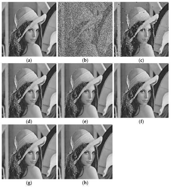
Figure 4.
Denoising results of different methods for image with 70% noise density (Lena). (a) Original image; (b) noisy image; (c) WMF; (d) AMF; (e) AWMF; (f) literature [16]; (g) literature [17]; (h) ours.
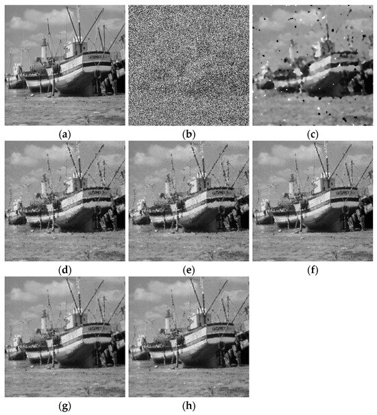
Figure 5.
Denoising results of different methods for image with 80% noise density (Boat). (a) Original image; (b) noisy image; (c) WMF; (d) AMF; (e) AWMF; (f) literature [16]; (g) literature [17]; (h) ours.
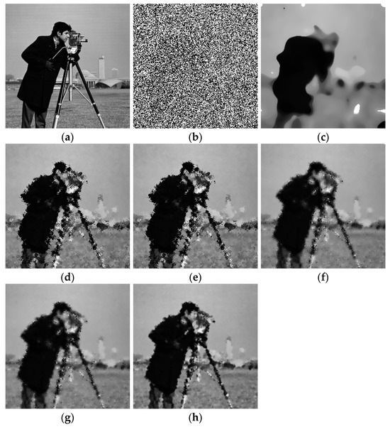
Figure 6.
Denoising results of different methods for image with 90% noise density (C.man). (a) Original image; (b) noisy image; (c) WMF; (d) AMF; (e) AWMF; (f) literature [16]; (g) literature [17]; (h) ours.
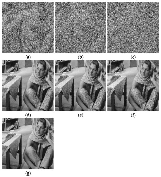
Figure 7.
The denoising results of our method for the same image with different noise densities. (a) 70%; (b) 80%; (c) 90%; (d) 70% (23.21/0.7520); (e) 80% (22.69/0.7064); (f) 90% (22.04/0.6429); (g) original image.
To test the denoising efficiency of this algorithm in high-density noise, six images of size 256 × 256 were selected for the experiments, and the average running times of different algorithms were shown in Table 5. Although the run times of the AMF and AWMF were shorter than the run time of this paper’s method, this paper’s method achieved a balanced performance by virtue of its better denoising effect. The efficiency of the method in this paper was better than that of the algorithm in the literature [16], and it was close to the computational speed of the method in the literature [17] in the high-noise scenes, which demonstrates the combined advantages of the algorithm in denoising effect and operational efficiency. However, for denoising scenarios with high real-time requirements, the efficiency of the algorithm proposed in this paper needs to be improved. In the future, analyzing the salt-and-pepper noise distribution prior (such as the sparsity) is expected to narrow the parameter search range of PSO and reduce the number of iterations. Alternatively, the run time can be further reduced and the efficiency of the algorithm improved by parallelizing the particle iteration process of PSO with the filtering process.
Table 5.
Average run time (S) for different methods.
4.2.2. Color Image Testing
To verify the denoising effectiveness of this paper’s method for color images, two representative color images (Lena, Barbara) from the Set14 standard color image dataset and three color images of real scenes (Parrots, Buildings, Fruits) were selected for experiments, as shown in Figure 8. In the experiments, SPN with densities of 70%, 80%, and 90% was added to the images, which were denoised using the method of this paper. The noisy images and denoising results are shown in Figure 9, Figure 10, Figure 11, Figure 12 and Figure 13. The results show that this method had a significant suppression effect on noise of different densities. The facial details in Lena, the fabric texture in Barbara, the head texture in Parrots, the outlines of buildings and scenery in Buildings, and the details of baskets in Fruits were still well preserved under high-density noise. The visual effects were clear and quantitative indexes such as PSNR and SSIM were high, which verified the effectiveness and robustness of the method.
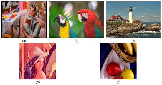
Figure 8.
Original images. (a) Barbara; (b) Parrots; (c) Buildings; (d) Lena; (e) Fruits.
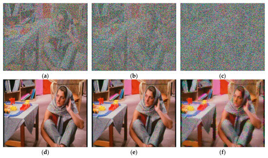
Figure 9.
Noisy image and denoising images (Barbara). (a) 70%; (b) 80%; (c) 90%; (d) 70% (23.25/0.8259); (e) 80% (22.17/0.7757); (f) 90% (19.79/0.6663).
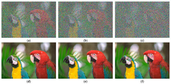
Figure 10.
Noisy image and denoising images (Parrots). (a) 70%; (b) 80%; (c) 90%; (d) 70% (27.12/0.9416); (e) 80% (25.61/0.9219); (f) 90% (23.80/0.8831).
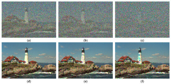
Figure 11.
Noisy image and denoising images (Buildings). (a) 70%; (b) 80%; (c) 90%; (d) 70% (22.85/0.8050); (e) 80% (21.66/0.7515); (f) 90% (20.26/0.6908).
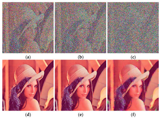
Figure 12.
Noisy image and denoising images (Lena). (a) 70%; (b) 80%; (c) 90%; (d) 70% (27.83/0.9657); (e) 80% (26.25/0.9504); (f) 90% (22.72/0.9101).
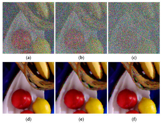
Figure 13.
Noisy image and denoising images (Fruits). (a) 70%; (b) 80%; (c) 90%; (d) 70% (28.17/0.9406); (e) 80% (25.72/0.9053); (f) 90% (24.54/0.8690).
5. Conclusions and Outlook
This paper proposed a hybrid decision-making adaptive median filtering algorithm integrating a dual-window detection mechanism and PSO to improve the inherent defects of the MF in image denoising, i.e., the blurring of edges caused by the fixed window and the limitations of manually setting the maximum window parameter of the AMF, as well as its insufficient ability to retain details under the high-density pepper noise.
This method constructed a hierarchical noise detection model. First, a 3 × 3 small window was utilized to quickly locate suspected noise points. The accuracy of noise recognition was further enhanced by a 5–35-pixel large window dynamically optimized by PSO, solving the problem that traditional methods rely on manual parameter adjustment. In the noise processing stage, the algorithm introduced a hybrid decision-making model based on the statistical characteristics of local pixels. It intelligently selected median filtering, spatial distance weighted averaging, or pixel retention operations according to the features of the neighborhood structure, effectively balancing the intensity of noise suppression and the degree of image detail retention. In addition, the PSO algorithm was used to globally optimize the large window’s size parameters, achieving full-process automation from noise detection to parameter adjustment, significantly reducing the cost of manual parameter adjustment. Experimental results showed that, in the case of high-density salt-and-pepper noise, the PSNR and SSIM of the proposed algorithm had significant improvements relative to other compared methods. Especially when dealing with images containing complex textures, it can effectively suppress the SPN while preserving image edges and texture features, avoiding the over-smoothing problem common to traditional methods. This research provides a solution that is both robust and adaptable for image preprocessing in high-noise environments such as medical images and remote sensing data, demonstrating potential to enhance image quality and the accuracy of subsequent analysis in practical applications.
In the future, the algorithm can be extended to scenarios such as Gaussian noise and mixed noise. By analyzing the statistical characteristics of different types of noise, the detection mechanism can be optimized to make the parameter optimization of PSO more targeted. Meanwhile, we can explore combining the algorithm with deep learning models. By leveraging their ability to acquire global image features, deep learning models can assist in window size selection and filtering decisions, further enhancing processing effects in complex noise environments.
Author Contributions
Conceptualization, J.M. and L.S.; methodology, J.M.; writing—original draft preparation, J.M. and J.C.; writing—review and editing, J.M. and J.C.; funding acquisition, J.C. and L.S. All authors have read and agreed to the published version of the manuscript.
Funding
This work was supported by the National Natural Science Foundation of China (grant #: 12174004) and the Ankang College Educational Teaching Reform Program (grant #: YJRG202503).
Institutional Review Board Statement
Not applicable.
Informed Consent Statement
Not applicable.
Data Availability Statement
Data are contained within the article.
Acknowledgments
The authors would like to thank the anonymous reviewers for their valuable comments.
Conflicts of Interest
The authors declare no conflicts of interest.
References
- Azzeh, J.; Zahran, B.; Alqadi, Z. Salt and pepper noise: Effects and removal. JOIV Int. J. Inform. Vis. 2018, 2, 252–256. [Google Scholar] [CrossRef]
- Jin, Y.Y.; Han, X.W.; Zhou, S.N. A review of image enhancement algorithms. Comput. Syst. Appl. 2021, 30, 18–27. [Google Scholar]
- Chen, P.Y.; Lien, C.Y. An efficient edge-preserving algorithm for removal of salt-and-pepper noise. IEEE Signal Process. Lett. 2008, 15, 833–836. [Google Scholar] [CrossRef]
- Zhang, X.; Xiong, Y. Impulse noise removal using directional difference based noise detector and adaptive weighted mean filter. IEEE Signal Process. Lett. 2009, 16, 295–298. [Google Scholar] [CrossRef]
- Gupta, V.; Chaurasia, V.; Shandilya, M. Random-valued impulse noise removal using adaptive dual threshold median filter. J. Vis. Commun. Image Represent. 2015, 26, 296–304. [Google Scholar] [CrossRef]
- Chan, R.H.; Ho, C.-W.; Nikolova, M. Salt-and-pepper noise removal by median-type noise detectors and detail-preserving regularization. IEEE Trans. Image Process. 2005, 14, 1479–1485. [Google Scholar] [CrossRef]
- Tyan, S.G. Median filtering: Deterministic properties. In Two-Dimensional Digital Signal Prcessing II: Transforms and Median Filters; Springer: Berlin/Heidelberg, Germany, 2006; Volume 43, pp. 197–217. [Google Scholar]
- Yang, Z.W.; Zheng, L.L.; Qu, H.S. Research on noise reduction algorithm of joint mean filtering and Poisson kernel bilateral filtering. Comput. Simul. 2020, 37, 460–463. [Google Scholar]
- Goel, N.; Kaur, H.; Saxena, J. Modified decision-based unsymmetric adaptive neighborhood trimmed-mean filter for removal of very high-density salt and pepper noise. Multimed. Tools Appl. 2020, 79, 19739–19768. [Google Scholar] [CrossRef]
- Brownrigg, D.R. The weighted median filter. Commun. ACM 1984, 27, 807–818. [Google Scholar] [CrossRef]
- Wang, Y.; Wang, J.; Song, X.; Han, L. An efficient adaptive fuzzy switching weighted mean filter for salt-and-pepper noise removal. IEEE Signal Process. Lett. 2016, 23, 1582–1586. [Google Scholar] [CrossRef]
- Hwang, H.; Haddad, R.A. Adaptive median filters: New algorithms and results. IEEE Trans. Image Process. 1995, 4, 499–502. [Google Scholar] [CrossRef]
- Riji, R.; Pillai, K.A.S.; Nair, M.S.; Wilscy, M. Fuzzy-based directional weighted median filter for impulse noise detection and reduction. Fuzzy Inf. Eng. 2012, 4, 351–369. [Google Scholar]
- Wang, W.; Du, W.; Li, Y.; Jia, Z. Advanced Adaptive Median Filter for Reducing Salt-and-Pepper Noise in GPR Data. IEEE Geosci. Remote Sens. Lett. 2025, 22, 3532986. [Google Scholar] [CrossRef]
- Guo, H.J.; Bai, W.J. Adaptive iterative mean filtering algorithm for removing image pretzel noise. J. Taiyuan Coll. (Nat. Sci. Ed.) 2020, 38, 23–28. [Google Scholar]
- Zhang, J.S.; Chen, M.J.; Xiong, X.Z. An adaptive nonlocal mean filter for removing pretzel noise. J. Sichuan Univ. Sci. Eng. (Nat. Sci. Ed.) 2022, 35, 59–65. [Google Scholar]
- Li, Z.X.; Yang, Y.; Huang, S.S.; Zhao, X.H.; Dong, Y.Y. Research on the fusion algorithm of mean and fast median filtering with adaptive weights. Comput. Digit. Eng. 2024, 52, 700–704. [Google Scholar]
- Fu, B.; Zhao, X.; Li, Y.; Wang, X.; Ren, Y. A convolutional neural networks denoising approach for salt and pepper noise. Multimed. Tools Appl. 2019, 78, 30707–30721. [Google Scholar] [CrossRef]
- Putra, B.P.E.; Prasetyo, H.; Suryani, E. Residual Transformer Fusion Network for Salt and Pepper Image Denoising. arXiv 2025, arXiv:2502.09000. [Google Scholar]
- Rafiee, A.A.; Farhang, M. A deep convolutional neural network for salt-and-pepper noise removal using selective convolutional blocks. Appl. Soft Comput. 2023, 145, 110535. [Google Scholar] [CrossRef]
- Siddique, M.F.; Saleem, F.; Umar, M.; Kim, C.H.; Kim, J.-M. A Hybrid Deep Learning Approach for Bearing Fault Diagnosis Using Continuous Wavelet Transform and Attention-Enhanced Spatiotemporal Feature Extraction. Sensors 2025, 25, 2712. [Google Scholar] [CrossRef]
- Zhou, J.X.; Zhou, F.Q. Wavelet denoising analysis based on improved cooperative quantum particle swarm optimization. Electron. Opt. Control. 2022, 29, 47–50. [Google Scholar]
- Hassan, F.; Rahim, L.A.; Mahmood, A.K.; Abed, S.A. A hybrid particle swarm optimization-based wavelet threshold denoising algorithm for acoustic emission signals. Symmetry 2022, 14, 1253. [Google Scholar] [CrossRef]
- Jain, M.; Saihjpal, V.; Singh, N.; Singh, S.B. An Overview of Variants and Advancements of PSO Algorithm. Appl. Sci. 2022, 12, 8392. [Google Scholar] [CrossRef]
- Elsayed, E.K.; Salem, D.R.; Aly, M. A Fast Quantum Particle Swarm Optimization Algorithm for Image Denoising Problem. Int. J. Intell. Eng. Syst. 2020, 13, 98–112. [Google Scholar] [CrossRef]
- Wang, G.; Guo, S.; Han, L.; Cekderi, A.B.; Song, X.; Zhao, Z. Asymptomatic COVID-19 CT image denoising method based on wavelet transform combined with improved PSO. Biomed. Signal Process. Control. 2022, 76, 103707. [Google Scholar] [CrossRef]
- Garncarek, Ł.; Powalski, R.; Stanisławek, T. LAMBERT: Layout-aware language modeling for information extraction. In Proceedings of the International Conference on Document Analysis and Recognition, Lausanne, Switzerland, 5–10 September 2021; pp. 532–547. [Google Scholar]
- Loupas, T.; McDicken, W.N.; Allan, P.L. An adaptive weighted median filter for speckle suppression in medical ultrasonic images. IEEE Trans. Circuits Syst. 2002, 36, 129–135. [Google Scholar] [CrossRef]
Disclaimer/Publisher’s Note: The statements, opinions and data contained in all publications are solely those of the individual author(s) and contributor(s) and not of MDPI and/or the editor(s). MDPI and/or the editor(s) disclaim responsibility for any injury to people or property resulting from any ideas, methods, instructions or products referred to in the content. |
© 2025 by the authors. Licensee MDPI, Basel, Switzerland. This article is an open access article distributed under the terms and conditions of the Creative Commons Attribution (CC BY) license (https://creativecommons.org/licenses/by/4.0/).