Article

A Modified Nonlocal Macro–Micro-Scale Damage Model for the Simulation of Hydraulic Fracturing

Department of Engineering Mechanics, Hohai University, Nanjing 210098, China
*
Author to whom correspondence should be addressed.
Modelling 2025, 6(3), 58; https://doi.org/10.3390/modelling6030058
Submission received: 12 May 2025 / Revised: 17 June 2025 / Accepted: 18 June 2025 / Published: 26 June 2025

Abstract

The nonlocal macro–meso-scale damage (NMMD) model, implemented in the framework of the finite element method, has been demonstrated to be a promising numerical approach in simulating crack initiation and propagation with reliable efficacy and high accuracy. In this study, the NMMD model was further enhanced by employing an identical degradation mechanism for both the tensile and shear components of shear stiffness, thereby overcoming the limitation of equal degradation in shear and tensile stiffness inherent in the original model. Additionally, a more refined and physically sound seepage evolution function was introduced to characterize the variation in permeability in porous media with geometric damage, leading to the development of an improved NMMD model suitable for simulating coupled seepage–stress problems. The reliability of the enhanced NMMD model was verified by the semi-analytical solutions of the classical KGD problem. Finally, based on the modified NMMD model, the effects of preset fracture spacing and natural voids on hydraulic fracture propagation were investigated.

1. Introduction

Hydraulic fracturing plays a pivotal role in oil and shale gas extraction, offering significant value in enhancing hydrocarbon production. The fundamental principle of hydraulic fracturing is to inject a high-pressure water or water-based solution containing proppants and chemical additives into the target rock layer. When the injection pressure exceeds the tensile strength of the rock, fractures initiate and propagate within the rock matrix, forming a complex network of fractures. These cracks greatly increase the permeability of the rock, enabling the efficient release of previously inaccessible hydrocarbon resources. Therefore, a comprehensive understanding of fracture propagation mechanics is essential for optimizing hydraulic fracturing operations and maximizing hydrocarbon recovery.
To clarify the mechanism of rock fracture development in hydraulic fracturing, scholars have conducted extensive experimental, theoretical, and numerical simulations. In terms of experiments, all have been based on a true triaxial hydraulic fracturing test system [1,2,3,4], and the effects of stress difference, perforation pattern (perforation angle, perforation cluster number, number of perforations per cluster), crack initiation position, fracturing fluid viscosity, injection rate, and natural fractures on crack propagation in limestone samples [1], layered samples composed of natural sandstone and coal [2], and raw coal samples have been studied [3]. However, indoor experiments are often limited by conditions, scale, and cost, making it difficult to observe the real-time propagation process of cracks. In addition, current theoretical research often idealizes basic assumptions, making it difficult to accurately reflect the complex mechanisms of the hydraulic fracturing process. Therefore, numerical simulation methods are widely used in the study of hydraulic fracturing problems.
The numerical methods for simulating crack propagation are mainly divided into two broad categories: the discrete approach, based on fracture mechanics, and the smeared (spatially continuous) approach, based on damage mechanics. The former not only needs to provide crack propagation criteria by calculating fracture mechanics indicators such as stress intensity factor and J-integral, but also to solve the problem of mesh topology changes during crack propagation. Therefore, the calculation process is relatively cumbersome, whether it uses the finite element method (FEM), which continuously reconstructs the mesh [5,6]; the extended finite element method (XFEM) [7,8,9], which does not require mesh reconstruction but needs to update enrichment degrees of freedom; or the discrete element method (DEM), which can only fracture along discrete elements [10,11,12,13,14,15]. The DEM does not require a direct criterion for crack extension and can simulate crack propagation on a fixed mesh. However, cracks are presented in a smeared manner and it is difficult to obtain the crack width, meaning that the cubic law for fracture flow cannot be used in hydraulic fracturing simulation. Therefore, this type of crack simulation method based on smearing, such as peridynamics [16,17,18,19,20,21], the phase field method [22,23,24,25,26,27,28], and the nonlocal macro–micro-scale consistent damage (NMMD) method [29,30,31,32,33,34], faces challenges in simulating fracture flow during hydraulic fracturing.
Peridynamics, which has recently flourished, has attracted widespread attention due to its advantage of the natural generation of complex cracks, especially when involving the simulation of crack initiation, branching, or convergence. Faced with the coupling problem between fracture flow pressure and fracture width during hydraulic fracturing, Qin Mingqi et al. [35,36] achieved a fracture flow coupling simulation of hydraulic fracturing based on bond-based peridynamics by using the damage separation criterion of material point and obtaining crack width data from the relative displacement along the perpendicular direction of the crack of material points on both sides of the crack. However, the computational efficiency and accuracy of peridynamics are relatively low [19], and accuracy improvement requires the use of more time-consuming, bond-associated, state-based peridynamics [37] or peridynamics with high-order differential operators [18,19], resulting in a higher cost for the accurate calculation of crack width. Another popular method for simulating crack propagation, the phase field model, directly treats the phase transition caused by fracture as a variational variable in the calculation of the minimum value of the energy function [22,23], and considers the gradient effect of phase transition in the energy dissipation of crack formation, which localizes cracks in the form of damage. Faced with the problem of calculating crack width in hydraulic fracturing, Santillán et al. [37,38,39] approximated the crack width of a section perpendicular to the fracturing direction by integrating the inner product of displacement and damage phase gradient to obtain displacement jumps, enabling the fracture phase field method to capture the interaction between fracture flow and deformation during hydraulic fracturing. Zhuang et al. [40,41] avoided calculating the displacement jumps of hydraulic fracturing and treated the fracture as a highly permeable porous medium, using the seepage–stress coupling model of porous media to simulate fracture flow, in which the permeability of the fractured area increased linearly with the damage value, representing the phase transition. However, the linearized permeability model is only applicable to those areas within the damage threshold range, ignoring the permeability changes with damage in minor damage areas. The permeability of severely damaged areas is directly equal to that of completely fractured areas, making Zhuang’s model somewhat rough.
Due to the finite element framework, the computational efficiency and accuracy of the phase field method are higher than those of peridynamics. However, in the phase field model of hydraulic fracturing, involving three fields of hydra–mechanical–phase coupling, both the monolithic solution scheme and the staggered solution scheme still require a large amount of computation. Recently, Lu and Chen [30] proposed a nonlocal macro–meso-scale consistent damage (NMMD) model by combining the basic ideas of fracture phase field theory and peridynamics, providing a new perspective on the simulation of crack propagation. In the NMMD model, the microstructure of any point in a material is considered a nonlocal architecture composed of massive bonds surrounding that point, and the initiation and propagation of cracks are caused by continuous bond breakage at the meso-scale. The degradation of stiffness of that point is further determined by its geometric damage, which is evaluated using the weighted average of the bond damage around that point within a certain range. The NMMD model can reflect size effects, has no mesh dependence [30], and can simulate the possible bifurcation phenomenon of dynamic cracks [31]. Moreover, the theoretical system of the NMMD model is complete and self-consistent [42], involving the characteristic length calibration [43] and the intrinsic relationship between energy degradation mode and characteristic length [33], which can reveal the dependence of fracture toughness and fracture energy on the initial crack size [43]. Most importantly, it has been shown [44] that the computational efficiency and accuracy of the NMMD method are much higher than those of the fracture phase field method and peridynamics, especially after optimizing nonlocal architecture [32]. In addition, given the simple construction pattern of the NMMD model, it can be easily extended to the failure simulation of layered rocks by defining the critical elongation rate as an elliptical distribution function with direction [34], and to the failure simulation of complex stress states by introducing the nonlocal structured strain and decomposing it into volume expansion and deviation [44,45].
Based on the consideration of the above advantages of the NMMD method in simulating crack propagation, this method is applied in this study to simulate hydraulic fracturing, and the fracture flow is treated as a highly permeable porous medium. In contrast to Zhuang’s model [40,41] and displacement-jump-based approaches [37,38,39] in the phase field model, this study aims to extend the NMMD model in simulating hydraulic fracturing problems with a balance between the relatively rational evolution of permeability with respect to damage and the sophisticated algorithm dealing with displacement jumps.
The structure of this paper is as follows: Section 2 briefly introduces the fundamental theory of the NMMD model, which overcomes the issue of equal degradation in shear and tensile stiffness present in the original model. Section 3 elaborates on the improved NMMD model for hydraulic fracturing in porous media by incorporating the seepage evolution function. In Section 4, three numerical examples are presented to demonstrate the reliability and advantages of the enhanced NMMD method. Finally, Section 5 summarizes the study and discusses the relevant conclusions.

2. Brief Summary of NMMD Model

In the NMMD model [30], the material microstructure is represented as a nonlocal network of multiple bonds originating from a single point. Crack formation and growth occur through progressive bond rupture at the meso-scale. Therefore, the geometric damage, reflecting the loss of continuity at the macroscale, can be quantified by weighting the sum of the related bond damage. As bond breakage continues, material stiffness progressively degrades. Consequently, stiffness reduction can be determined from the point-wise damage resulting from bond failure.

2.1. Microstructural-Scale Damage

Consider a spatial entity Ω d d { 1 , 2 , 3 } represented by boundary Ω , and use spatial coordinates x = x 1 , , x d and x = ( x 1 , , x d ) . to distinguish the material points inside it. The material point pairs can be defined as
N : = { ( x , x ) Ω × Ω L ( x , x ) Ω = , x x }
Among them, L x , x is a line segment determined by a pair of material points x and x . For any material point x , the nonlocal structure of its material point is shown in Figure 1, where l represents the characteristic length [46].
For the microstructural lever, define the deformation rate of material point pairs as
λ ( x , x , t ) = 1 | ξ | ( u ( x , t ) u x , t ) ν
where ξ is the bond vector from x to x , | ξ | is the corresponding bond length, ν = ξ / | ξ | is the corresponding unit bond vector, and u x , t and u ( x , t ) are the displacement of point x and x at time t, respectively. The stretch rate is further defined as
λ + ( x , x , t ) = λ ( x , x , t ) H ( λ ( x , x , t ) )
where H is Heaviside step function. When λ < 0 , H λ = 0 , otherwise H λ = 1 . Once the stretch rate surpasses critical threshold λ c , the pairwise interaction between points progressively diminishes until it fully vanishes. To model this irreversible behavior, a history-dependent parameter κ is introduced, representing the maximum attained elongation rate during loading. Specifically, this is expressed as
κ ( x , x , t ) = max τ 0 , t λ + x , x , τ λ c , 0 , ( x , x ) N
where t represents the time, or virtual time for the static problem, κ = 0 corresponds to the elastic phase, and κ denotes full material separation. Consequently, the micro-scale damage ω ( x , x , t ) 0 , 1 is formulated as an exponential function of the historically attained peak stretch rate.
ω ( x , x , t ) ω ^ ( x , x , t ) = 1 exp γ κ
where γ is a material brittleness index reflecting the brittleness degree. When κ = 0 , ω ( x , x , t ) = 0 , meaning that the bond is in an intact state. The damage to material bonds develops with the increase of κ . When κ increases to a certain value, the material point pair is completely damaged.

2.2. Geometric Damage Reflecting Macro-Scale Continuity Loss and Free Energy Damage Reflecting Stiffness Degradation

The macroscopic damage state of a material point is characterized by geometric damage d ω x , t , computed as the weighted mean of microstructural damage values ω across all connected point pairs to x .
d ω x , t = D l x φ ( x , x ) ω ( x , x , t ) d V
where d V = V d ( x ) is the Lebesgue measure, and φ ( x , x ) + is the influence function.
Geometric-based damage directly quantifies material degradation through microscopic defects such as crack density and porosity, while energy-based damage describes the energy dissipation required for damage evolution from a thermodynamic perspective. The essential correlation between the two lies in the fact that the propagation of geometric defects is driven by energy (such as the need to overcome surface energy for crack propagation), and energy dissipation depends on the geometric distribution of defects. From damage mechanics principles, the progression of geometric damage necessarily results in free energy density redistribution. This energy dissipation mechanism can be mathematically represented through the degradation function g d ω , formulated as
g d ω = 1 ψ 0 ε ψ ε , d ω
where ψ ε , d ω is the Helmholtz free energy, ε = S u is the strain tensor, S is the symmetric gradient operator, and ψ 0 is the energy density function of the material without damage.
ψ 0 ε = 1 2 ε : E : ε
where E is the fourth-order elastic stiffness tensor.
Due to the irreversibility of damage, the energy degradation function table should clearly exhibit a monotonic decrease. Therefore, g d ω , which represents the deformation energy storage capacity of any material point, needs to meet the requirements
g 0 = 1 , g 1 = 0 d d ω g < 0 , d d ω g 1 = 0
where g 0 = 1 indicates the material point is in an undamaged state, and g 1 = 0 indicates the material’s ability to store deformation energy is completely lost; d d ω g < 0 means that the damage reflects a process of energy dissipation; when d ω = 1 , it means that there is no damage-driving force provided. Therefore, as energy is released, the force driving the development of damage becomes smaller, leading to the conclusion that the free energy damage Φ is always greater than the geometric damage of d ω [28], i.e.,
Φ = 1 g d ω > d d d ω g d ω < 1
Thus, the energy degradation factor of this model can be constructed as the convex function [30]
g d ω = 1 d ω p 1 + q 1 1 d ω p , p > 1 , q > 0
where p and q are parameters controlling the energy dissipation rate.

2.3. Nonlocal Damage Constitutive Model for Tensile or Tensile–Shear Fracture

Considering that the hydraulic fracturing process is mainly dominated by tensile or tensile–shear failure, this study only focuses on the degradation of deformation stiffness that reflects tensile or tensile–shear. The strain tensor ε can be decomposed into tensile and compressed parts
ε + = a = 1 3 ε a + n a n a ε = a = 1 3 ε a n a n a
where ε + and ε are tension and compression strain tensor, respectively; ε a is the principal strain; and n a is the corresponding principal direction. Operators · + and · are defined as · + = + / 2 and · = / 2 . For isotropic material, the strain energy density in tension and compression can be obtained as
ψ ε + ε = λ 2 tr ε + 2 + ϑ tr ε + 2 ψ ε ε = λ 2 tr ε 2 + ϑ tr ε 2
where λ is the Lame constant, ϑ is the shear modulus, and tr denotes the trace operator. Thus, the elastic strain energy density is expressed as
ψ ε ε = g d w ψ ε + ε + ψ ε ε
Therefore, the nonlocal damage constitutive equation can be given as
σ = g d w ψ ε + ε + ψ ε ε = g d w λ tr ε + I + 2 ϑ ε + + λ tr ε I + 2 ϑ ε
where I is a unit tensor.

3. Modified NMMD Model for Hydraulic Fracture in Porous Media

In this section, the evolution of the permeability field related to geometric damage in the NMMD model is introduced, starting from the evolution of the permeability field in porous media, which is an irreversible process of growth. Then, the momentum equilibrium equation of the NMMD model and the mass balance of fluid is coupled with the Darcy seepage law, endowing the damaged permeability field and forming the governing equations of the proposed extended NMMD model for simulating hydraulic fracture problems. Details of the weak form and numerical implementation of the proposed model are also given.

3.1. Fluid Flow in the Isotropic Medium

For porous media such as rock or concrete, geometric damage reflecting the loss in continuity directly affects the permeability of the medium. It is assumed that the fluid in porous media is compressible and viscous. The porous medium domain can be decomposed into three parts: the reservoir domain, the transition domain, and the fracture domain. In the reservoir domain, the permeability is not significantly affected by geometric damage, while in the transition domain, the permeability increases linearly with the development of geometric damage. In the fractured domain, the permeability coefficient gradually tends towards a stable value for a complete cracked state. Therefore, the evolution law of the medium permeability coefficient with geometric damage can be constructed as
k = f d w k 0 = k f k 0 k 0 d w α sin 2 π d w 2 π + 1 k 0
where f d w is the seepage evolution factor, k 0 is the permeability coefficient of the intact zone, k f is the permeability coefficient of the completely fractured domain, and α 0 , 1 is an interpenetrating parameter, reflecting the sensitivity of permeability growth due to spatial discontinuity. Figure 2 shows the variation in permeability evolution with respect to geometric damage d ω for different interpenetrating parameters. When α 0 , the permeability evolves linearly with the geometric damage.

3.2. Governing Equations

The hydraulic fracturing process in porous media can be regarded as a quasi-static problem. Assuming that the medium is always in a saturated state during hydraulic fracturing, the equilibrium equation for porous media is given as
σ + ρ b = 0 σ β p I + ρ b = 0
where ρ is the density of the mixture, β is the Biot coefficient, b is the body force b = 0 g T , for the plane problem, and b = 0     0 g T for three dimension problem; here, g is the gravity acceleration. Assuming that the fluid flow during hydraulic fracturing follows Darcy’s law,
q = k ν p + ρ f b
where ν is the viscosity of the fluid, k denotes the permeability tensor, and for the isotropic medium, k = f d w k 0 I . ρ f denotes the density of the fluid. From the flow balance condition, the seepage equation can be obtained as
q + 1 Q p ˙ + β ε ˙ v = 0 k ν p + ρ f b + 1 Q p ˙ + β ε ˙ v = 0
where q represents the seepage density vector, Q is the compression modulus of the fluid, and β ε ˙ v denotes the drainage caused by the volume compression of the medium. Here, ε v is the volume strain. The displacement u p and pore pressure p p for any a point p x , t can be gained by the shape function interpolation of the element, as follows:
u N = N u u e p N = N p p e
Here, N u and N p are the displacement and pore pressure interpolation shape function matrix, respectively. u e and p e are the nodal displacement and nodal pore pressure in an element, respectively.
The equilibrium Equation (19) can be discretized using the standard Galerkin method as
Λ N e e = 1 Ω e g d w B u T DB u d Ω u Λ N e e = 1 Ω e β B u T m N u d Ω p = Λ N e e = 1 Ω e N u T ρ b d Ω + Λ N e e = 1 Γ e N u T f ¯ d Ω Λ N e e = 1 Ω e β B u T m N p d Ω u ˙ + Λ N e e = 1 Ω e 1 Q N p T N p d Ω p ˙ + Λ N e e = 1 Ω e B p T k d w ν B p d Ω p = Λ N e e = 1 Ω e B p T k d w ν ρ f b d Ω
where Λ N e e = 1 is the elemental assemble operator, and u and p are the total nodal displacement vector and the total nodal pore pressure vector, respectively. B u is the strain matrix and B p is the pore pressure gradient matrix. Their corresponding subarrays B u i and B p i for elemental node i are
B u i = N u i x 0 0 N u i y N u i y N u i x ; B u i = N p i x N p i y
and ε v = m T ε = m T B u u is used; here, m is the vector of the delta Dirac function defined as m = 1   1   0 T for the plane strain problem or axisymmetric problem.
Let K = Λ N e e = 1 Ω e g d w B u T D B u d Ω , Q = Λ N e e = 1 Ω e B u T m N p d Ω , S = Λ N e e = 1 Ω e 1 Q N p T N p d Ω , R u = Λ N e e = 1 Ω e N u T ρ b d Ω + Λ N e e = 1 Γ e N u T f ¯ d Ω , H = Λ N e e = 1 Ω e B p T k d w ν B p d Ω , R p = Λ N e e = 1 Ω e B p T k d w ν ρ f b d Ω
Then, the seepage–stress coupling Equation (23) can be simplified as
K u Q p = R u Q u ˙ + S p ˙ + H p = R p

4. Numerical Examples

4.1. Verification: KGD Hydraulic Fracturing Problem

Shown in Figure 3 are the geometry, injection, and constrained boundary conditions of the KGD hydraulic fracturing problem. Both L 1 and L 2 are 10.0 m, and the prescribed displacement and pressure of the surrounding boundaries are set to zero (i.e., permeable boundaries). The pre-existing crack length l p r e = 1.0   m , and the water injection rate is Q = 2 × 10 4   m 2 /s, while the time step Δ t = 0.01   s . The parameters p and q in the energetic degradation function [30] are set to 3 and 4, respectively, while the interpenetrating parameter α is set to 0.4, and the other relevant material parameters are shown in Table 1.

4.1.1. Convergence of Mesh Sizes with Semi-Analytical Solution

As is well known, the KGD problem is widely used for the validation of hydraulic fracturing models. A semi-analytical solution [47,48] to this problem was obtained by assuming that the fluid inside the crack is incompressible, ignoring the actual injection pressure path prior to hydraulic crack propagation, namely
L c = 0.65 G Q 3 υ 1 μ t ,
where Q is the injection rate of fluid, G is the shear modulus, υ is the fluid viscosity, μ is Poisson’s ratio, and t 2 3 is the time. And the pressure of the fracturing fluid injected into the hole is
p = σ min + 0.96 2 G 3 Q υ 1 μ 3 L c 2 1 4 ,
where σ min is the minimum ground stress, which is set to zero here.
To investigate the convergence of the extended NMMD model, we first consider different sizes of finite element discretizations in solving Equation (23). In view of the deformation gradient at the crack front being too large during hydraulic fracturing, it is required that the mesh in the fracturing area be sufficiently dense to accurately track the hydraulic fracturing process. Therefore, this paper uses four different grid sizes for encryption in the potential crack propagation domain, i.e., h = 20 mm, 40 mm, 60 mm and 160 mm. Extracted from the numerical results of the extended NMMD model, the injection pressures within the crack under different mesh densities are shown in Figure 4. It can be seen that the numerical solution of the injection pressure gradually converges to the semi-analytical solution, namely Equations (24) and (25), as the minimum mesh size tends to zero. It should be pointed out that the linear component in the semi-analytical solution is the actual injection pressure path prior to hydraulic crack propagation. In other words, these results directly demonstrate that the extended NMMD model is robust and reliable in simulating the hydraulic fracturing process.

4.1.2. Influence of the Interpenetrating Parameter

As mentioned before, the geometry-based damage in the NMMD model is a physical quantity ranging from [0, 1] that reflects the degree of spatial discontinuity. In this subsection, we would like to discuss the influence of the interpenetrating parameter on the results of the extended NMMD model.
To this end, three cases of α = 0.40 , 0.45 and α = 0.50 are considered. Shown in Figure 5 are the corresponding variations in injection pressure within crack interior and crack propagation length with respect to injection time. As can be seen in Figure 5a, before the injection pressure reaches its peak value, the interpenetrating parameter would control the increasing rate of injection pressure. Recalling the variation in permeability evolution factor with geometry-based damage in Figure 2, minor damages are insufficient to cause a significant increase in the permeability coefficient at a small interpenetrating parameter, resulting in the injection pressure increases at a faster rate when the value of the interpenetrating parameter is small. After the peak values of injection pressure, the larger the value of the interpenetrating parameters input, the smaller the response of the injection pressure output. In Figure 5b, on the other hand, one clearly sees that crack propagation lengths obtained using the extended NMMD model are very closed to the semi-analytical one, except for the stage before the critical cracking moment (about 0.8 s). This is because during the derivation of the semi-analytical solution, the time required for fluid injection was neglected, resulting in an infinite pressure at the beginning of the injection (see Figure 5a), which contradicts the real physical situation. In contrast, the extended NMMD model can capture actual behavior that occurs in the hydraulic crack initiation if and only if the injection pressure reaches its peak.
Shown in Figure 6 are the distributions of geometry-based damage at different stages, shown in Figure 5b, which reflect the process of the pre-existing crack gradually extending under hydraulic action.

4.1.3. Comparison with Phase Field Models

To verify the effectiveness of the extended nonlocal macro–micro-damage model constructed in this paper, we will compare the numerical results of the NMMD model based on seepage stress coupling with analytical solutions, and further compare them with the numerical results of other models to demonstrate the superiority of our model.
Shown in Figure 7 are the evolution of injection pressure and crack propagation length obtained by the extended NMMD model, phase field models based on the displacement-jump approach and endowed with the linearized permeability assumption, and the semi-analytical solutions. It can be seen that the numerical results of the extended NMMD model are more consistent with the semi-analytical solutions after the peak value of injection pressure than those of Zhuang’s model. This indicates that the evolution of permeability field with non-linearity, rather than linearity, adopted in the extended NMMD model is more capable of depicting the essential feature of hydraulic fracturing behavior. On the other side, the extended NMMD model shares almost the same accuracy with the displacement-jump-based phase field model in simulating the KGD problem. Unfortunately, the computational efficiency was not provided directly in [37]. However, in the extended NMMD model, there is no need to calculate the displacement jumps like Chukwudozie’s model does, which involves complicated and time-consuming algorithms. Moreover, it has been proven numerically that the CPU time of the NMMD model is merely one-tenth of that of phase field model for the same benchmark cracking problem with similar degrees of freedom and hardware. Therefore, it is reasonable to believe that the proposed extended NMMD model could provide a potential solution with its attractive computational efficiency in simulations of hydraulic fracturing of porous media.

4.2. Double-Fracture Hydraulic Fracturing with Different Spacing

The modified NMMD model based on constructed seepage–stress coupling was used to simulate the fracturing problem of multiperforated horizontal wells. The calculation model for the synchronous fracturing of multiperforated horizontal wells is shown in Figure 8a. Due to its geometric symmetry, we take the half structure for calculation, as shown in Figure 8b. The length of the model is 20.0   m , the height is 5.0   m , and the displacement and pressure on the boundary are both 0.0. The two preset crack lengths are all 1.0   m , with a spacing of d. The calculation is carried out using four-nodal isoparameter elements, with the main material parameters set as follows: elastic modulus E = 24.0 GPa, Poisson’s ratio ν = 0.2 , permeability coefficient in the undamaged area k 0 = 1 × 10 9  mm/s, permeability coefficient in the completely damaged area k f = 1 × 10 3  mm/s, viscosity coefficient υ = 0.001   MPa s , Biot coefficient β = 1.0 , and porosity n = 0.19 . The main calculation parameters are set as follows: energy degradation parameters p, q, and γ are 4, 15, and 2000, respectively; seepage evolution parameter α = 1.0 ; critical elongation rate λ c = 0.0001 ; and time incremental step Δ t = 0.01   s . The injection rate of fracturing fluid is Q = 3 × 10 2  m2/s.
The damage distribution of three different preset crack spacings after 2.0 s of liquid injection is shown in Figure 9. It can be seen that when the crack spacing is 4.0 m, the crack first expands along the preset direction by approximately 0.65 m and then expands outward at a 22° deflection angle. When the crack spacing is 6.0 m, the crack first expands along the preset direction by approximately 1.22 m and then expands outward at a deviation angle of 15°. When the crack spacing is 8.0 m, the cracks always propagate along the predetermined direction without deflection.
Figure 10 shows the variation curve of the average pressure at the tips of two preset cracks of different spacings as a function of injection time. It is not difficult to see that as the injection continues, the pressure at the tip of the preset crack increases, which, in turn, causes the crack to expand. After the crack begins to expand, the injected fracturing fluid can enter the expansion section, so the preset pressure at the crack tip decreases. For different distances between two cracks, the average pressure at the tip varies slightly over time. As the spacing increases, the peak pressure decreases. It can be seen that the crack propagation speed also varies. This proves that there is a mutual interference relationship between the two cracks, and this interference relationship weakens with the increase in spacing.

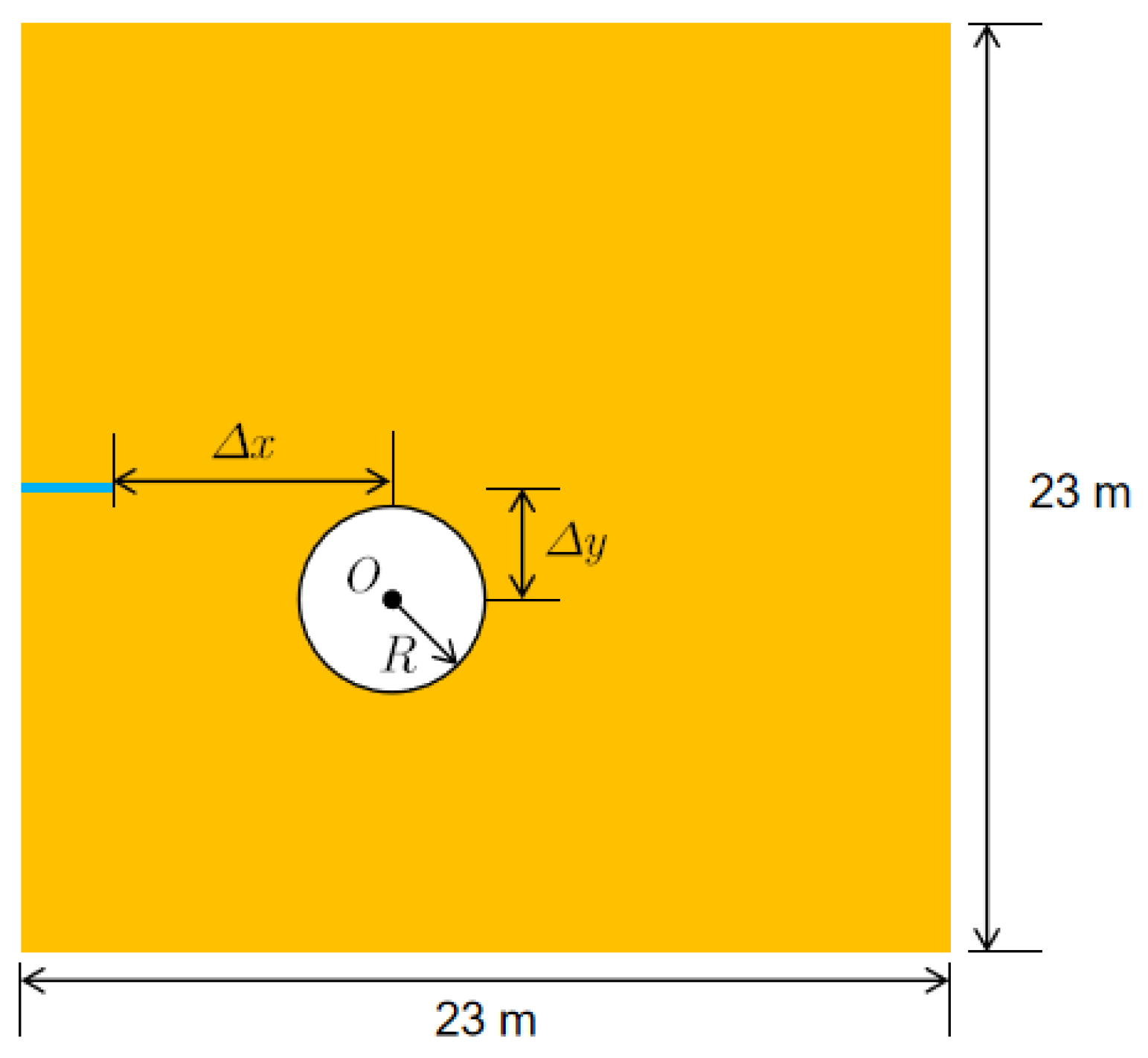
4.3. Hydraulic Fracturing with Natural Pores

In practical engineering, the problem of natural pores may be encountered during the hydraulic fracturing process of preset cracks. A two-dimensional model is shown in Figure 11. The model is a square with a side length of 23.0   m , and the preset crack length is 2.3   m . There is a natural hole within the square. The difference in the horizontal axis between the circular center and the preset crack tip is Δ x , and the corresponding difference in the vertical axis is Δ y . All four edges are fixed, and they are all permeable boundaries, that is, with a pressure of 0.0. The calculation is carried out using four-nodal isoparameter elements. The main material parameters are set as follows: elastic modulus E =   17.0   GPa , Poisson’s ratio ν = 0.2 , permeability coefficient in the undamaged area k 0 = 3.5 × 10 9 mm/s, permeability coefficient in the completely damaged area k f = 3.5 × 10 4 mm/s, viscosity coefficient υ = 0.001   MPa s , Biot coefficient β = 1.0 , and porosity n = 0.19 . The main calculation parameters are set as follows: energy degradation parameters p, q, and γ are 4, 15, and 2000, respectively; seepage evolution parameter α = 1.0 ; critical elongation rate λ c = 0.00015 ; and time step Δ t = 0.01   s . The injection rate of the fracturing fluid is Q = 1 × 10 2  m2/s.
To explore the influence of natural pores on the hydraulic fracturing path, the six cases listed in Table 2 were chosen according to the arrangement of the holes and their position and size. With the injection of fracturing fluid, after a period of time, the preset crack expands to intersect with the natural pores and further expands. The damage distributions under various cases are shown in Figure 12.
The damage paths of these cases show that natural pores have an inducing effect on the propagation of hydraulic fractures, even when the natural pores are small. With the continuous injection of fracturing fluid, new damage occurs when natural pores are filled with the fluid, ultimately forming new cracks. When a natural hole is basically level with the hydraulic fracture, cracks are evenly generated from the hole opening, and the number of generated cracks is large (such as in A, B, and E). However, when the natural hole is offset from the hydraulic fracture, only one crack (such as in C, D, and F) appears from the hole opening for fracturing. Furthermore, the smaller the size of the hole, the fewer the cracks generated by the water pressure in the filled hole after the hydraulic cracks merge with the natural hole.

5. Conclusions

In this study, we modified the macro–meso-scale consistent damage model (NMMD) proposed by Lu and Chen [30], where the tensile–shear part of shear stiffness is decomposed and weakened by the same degradation mechanism as tensile stiffness, overcoming the problem of the equal degradation of shear stiffness and tensile stiffness in the original model. Then, by introducing a more refined and physically sound seepage evolution function to describe the variation in the permeability of porous media with geometric damage, the NMMD model was extended to simulate coupled seepage–stress problems. And then, the reliability and rationality of the proposed extended NMMD model are verified using the semi-analytical solutions of the classical KGD problem. Finally, based on the improved NMMD model proposed in this study, two hydraulic fracturing scenarios in porous media were selected and simulated: dual-fracture hydraulic fracturing and hydraulic fracturing with natural voids. The effects of preset fracture spacing and natural voids on hydraulic fracture propagation were investigated. The numerical results once again demonstrate the advantages of the NMMD model, which requires no mesh reconstruction or fracture tracking techniques. Moreover, the enhanced NMMD model retains its significant computational efficiency, showing great potential for solving coupled problems.
It should be noted that the modified NMMD model in this study is not yet applicable to the numerical simulation of coupled problems in anisotropic porous media. Further improvements will be pursued in future research.

Author Contributions

Program implementation, Simulation, and Writing—original-draft, C.L.; Conceptualization, Methodology, and Writing—review and editing, X.X. All authors have read and agreed to the published version of the manuscript.

Funding

This research was funded by the National Natural Science Foundation of China (No. 11932006, 12202314).

Data Availability Statement

Dataset available on request from the authors.

Conflicts of Interest

The authors declare no conflicts of interest.

References

  1. Yang, W.; Geng, Y.; Zhou, Z.; Li, L.; Ding, R.; Wu, Z.; Zhai, M. True triaxial hydraulic fracturing test and numerical simulation of limestone. J. Cent. South Univ. 2020, 27, 3025–3039. [Google Scholar] [CrossRef]
  2. Tan, P.; Jin, Y.; Yuan, L.; Xiong, Z.-Y.; Hou, B.; Chen, M.; Wan, L.-M. Understanding hydraulic fracture propagation behavior in tight sandstone–coal interbedded formations: An experimental investigation. Pet. Sci. 2019, 16, 148–160. [Google Scholar] [CrossRef]
  3. Chen, D.; Li, N.; Sun, W. Rupture properties and safety assessment of raw coal specimen rupture process under true triaxial hydraulic fracturing based on the source parameters and magnitude. Process Saf. Environ. Prot. 2022, 158, 661–673. [Google Scholar] [CrossRef]
  4. Li, M.; Zhou, F.; Dong, E.; Zhang, G.; Zhuang, X.; Wang, B. Experimental study on the multiple fracture simultaneous propagation during extremely limited-entry fracturing. J. Petrol. Sci. Eng. 2022, 218, 110906. [Google Scholar] [CrossRef]
  5. Bao, J.Q.; Fathi, E.; Ameri, S. A coupled finite element method for the numerical simulation of hydraulic fracturing with a condensation technique. Eng. Fract. Mech. 2014, 131, 269–281. [Google Scholar] [CrossRef]
  6. Bao, J.Q.; Fathi, E.; Ameri, S. Uniform investigation of hydraulic fracturing propagation regimes in the plane strain model. Int. J. Numer. Anal. Methods Geomech. 2015, 39, 507–523. [Google Scholar] [CrossRef]
  7. Belytschko, T.; Black, T. Elastic crack growth in finite elements with minimal remeshing. Int. J. Numer. Methods Eng. 1999, 45, 601–620. [Google Scholar] [CrossRef]
  8. Gordeliy, E.; Peirce, A. Coupling schemes for modeling hydraulic fracture propagation using the XFEM. Comput. Methods Appl. Mech. Eng. 2013, 253, 305–322. [Google Scholar] [CrossRef]
  9. Li, J.; Dong, S.; Hua, W.; Yang, Y.; Li, X. Numerical Simulation on Deflecting Hydraulic Fracture with Refracturing Using Extended Finite Element Method. Energies 2019, 12, 2044. [Google Scholar] [CrossRef]
  10. Zhang, Q.; Wang, Z.; Xia, X. Interface stress element method and its application in analysis of anti-sliding stability of gravity dam. Sci. China Technol. Sci. 2012, 55, 3285–3291. [Google Scholar] [CrossRef]
  11. Yan, C.; Jiao, Y.-Y.; Zheng, H. A fully coupled three-dimensional hydro-mechanical finite discrete element approach with real porous seepage for simulating 3D hydraulic fracturing. Comput. Geotech. 2018, 96, 73–89. [Google Scholar] [CrossRef]
  12. Huang, L.; Liu, J.; Zhang, F.; Dontsov, E.; Damjanac, B. Exploring the influence of rock inherent heterogeneity and grain size on hydraulic fracturing using discrete element modeling. Int. J. Solids Struct. 2019, 176–177, 207–220. [Google Scholar] [CrossRef]
  13. Yang, W.; Li, S.; Geng, Y.; Zhou, Z.; Li, L.; Gao, C.; Wang, M. Discrete element numerical simulation of two-hole synchronous hydraulic fracturing. Geomech. Geophys. Geo-Energy Geo-Resour. 2021, 7, 55. [Google Scholar] [CrossRef]
  14. Deng, S.; Li, H.; Ma, G.; Huang, H.; Li, X. Simulation of shale–proppant interaction in hydraulic fracturing by the discrete element method. Int. J. Rock Mech. Min. Sci. 2014, 70, 219–228. [Google Scholar] [CrossRef]
  15. Marina, S.; Imo-Imo, E.K.; Derek, I.; Mohamed, P.; Yong, S. Modelling of hydraulic fracturing process by coupled discrete element and fluid dynamic methods. Environ. Earth Sci. 2014, 72, 3383–3399. [Google Scholar] [CrossRef]
  16. Silling, S.A. Reformulation of elasticity theory for discontinuities and long-range forces. J. Mech. Phys. Solids 2000, 48, 175–209. [Google Scholar] [CrossRef]
  17. Silling, S.A.; Epton, M.; Weckner, O.; Xu, J.; Askari, E. Peridynamic States Constitutive Modeling. J. Elast. 2007, 88, 151–184. [Google Scholar] [CrossRef]
  18. Gu, X.; Li, X.; Xia, X.; Madenci, E.; Zhang, Q. A robust peridynamic computational framework for predicting mechanical properties of porous quasi-brittle materials. Compos. Struct. 2023, 303, 116245. [Google Scholar] [CrossRef]
  19. Gu, X.; Zhang, Q.; Madenci, E.; Xia, X. Possible causes of numerical oscillations in non-ordinary state-based peridynamics and a bond-associated higher-order stabilized model. Comput. Methods Appl. Mech. Eng. 2019, 357, 112592. [Google Scholar] [CrossRef]
  20. Cao, C.; Gu, C.; Wang, C.; Wang, C.; Xu, P.; Wang, H. A Peridynamics-Smoothed Particle Hydrodynamics Coupling Method for Fluid-Structure Interaction. J. Mar. Sci. Eng. 2024, 12, 1968. [Google Scholar] [CrossRef]
  21. Zeleke, M.A.; Ageze, M.B. A Review of Peridynamics (PD) Theory of Diffusion Based Problems. J. Eng. 2021, 2021, 7782326. [Google Scholar] [CrossRef]
  22. Bourdin, B.; Francfort, G.A.; Marigo, J.-J. Numerical experiments in revisited brittle fracture. J. Mech. Phys. Solids 2000, 48, 797–826. [Google Scholar] [CrossRef]
  23. Miehe, C.; Welschinger, F.; Hofacker, M. Thermodynamically consistent phase-field models of fracture: Variational principles multi-field FE implementations. Int. J. Numer. Methods Eng. 2010, 83, 1273–1311. [Google Scholar] [CrossRef]
  24. Wu, J.-Y. A unified phase-field theory for the mechanics of damage and quasi-brittle failure. J. Mech. Phys. Solids 2017, 103, 72–99. [Google Scholar] [CrossRef]
  25. Xia, X.; Qin, C.; Lu, G.; Gu, X.; Zhang, Q. Simulation of Corrosion-Induced Cracking of Reinforced Concrete Based on Fracture Phase Field Method. Comput. Model. Eng. Sci. 2024, 138, 2257–2276. [Google Scholar] [CrossRef]
  26. Deogekar, S.; Vemaganti, K. A computational study of the dynamic propagation of two offset cracks using the phase field method. Eng. Fract. Mech. 2017, 182, 303–321. [Google Scholar] [CrossRef]
  27. Yang, J.; Kim, J. A phase-field method for two-phase fluid flow in arbitrary domains. Comput. Math. Appl. 2020, 79, 1857–1874. [Google Scholar] [CrossRef]
  28. Shen, R.; Waisman, H.; Guo, L. Fracture of viscoelastic solids modeled with a modified phase field method. Comput. Methods Appl. Mech. Eng. 2019, 346, 862–890. [Google Scholar] [CrossRef]
  29. Huang, D.; Lu, G.; Liu, Y. Nonlocal Peridynamic Modeling and Simulation on Crack Propagation in Concrete Structures. Math. Probl. Eng. 2015, 2015, 858723. [Google Scholar] [CrossRef]
  30. Lu, G.; Chen, J. A new nonlocal macro-meso-scale consistent damage model for crack modeling of quasi-brittle materials. Comput. Methods Appl. Mech. Eng. 2020, 362, 112802. [Google Scholar] [CrossRef]
  31. Lu, G.; Chen, J. Dynamic cracking simulation by the nonlocal macro-meso-scale damage model for isotropic materials. Int. J. Numer. Methods Eng. 2021, 122, 3070–3099. [Google Scholar] [CrossRef]
  32. Lv, W.; Lu, G.; Xia, X.; Gu, X.; Zhang, Q. Discrepancy-informed quadrature strategy for the nonlocal macro-meso-scale consistent damage model. Comput. Methods Appl. Mech. Eng. 2024, 432, 117315. [Google Scholar] [CrossRef]
  33. Lv, W.; Lu, G.; Xia, X.; Gu, X.; Zhang, Q. Energy degradation mode in nonlocal Macro-Meso-Scale damage consistent model for quasi-brittle materials. Theor. Appl. Fract. Mech. 2024, 130, 104288. [Google Scholar] [CrossRef]
  34. Xia, X.; Wang, X.; Lu, G.; Gu, X.; Lv, W.; Zhang, Q.; Ma, L. A new nonlocal macro-micro-scale consistent damage model for layered rock mass. Theor. Appl. Fract. Mech. 2024, 133, 104540. [Google Scholar] [CrossRef]
  35. Qin, M.; Yang, D. Numerical investigation of hydraulic fracture height growth in layered rock based on peridynamics. Theor. Appl. Fract. Mech. 2023, 125, 103885. [Google Scholar] [CrossRef]
  36. Qin, M.; Yang, D.; Chen, W.; Yang, S. Hydraulic fracturing model of a layered rock mass based on peridynamics. Eng. Fract. Mech. 2021, 258, 108088. [Google Scholar] [CrossRef]
  37. Chukwudozie, C.; Bourdin, B.; Yoshioka, K. A variational phase-field model for hydraulic fracturing in porous media. Comput. Methods Appl. Mech. Eng. 2019, 347, 957–982. [Google Scholar] [CrossRef]
  38. Santillán, D.; Juanes, R.; Cueto-Felgueroso, L. Phase Field Model of Hydraulic Fracturing in Poroelastic Media: Fracture Propagation, Arrest, and Branching Under Fluid Injection and Extraction. JGR Solid Earth 2018, 123, 2127–2155. [Google Scholar] [CrossRef]
  39. Yoshioka, K.; Naumov, D.; Kolditz, O. On crack opening computation in variational phase-field models for fracture. Comput. Methods Appl. Mech. Eng. 2020, 369, 113210. [Google Scholar] [CrossRef]
  40. Zhou, S.; Zhuang, X. Phase field modeling of hydraulic fracture propagation in transversely isotropic poroelastic media. Acta Geotech. 2020, 15, 2599–2618. [Google Scholar] [CrossRef]
  41. Zhuang, X.; Zhou, S.; Sheng, M.; Li, G. On the hydraulic fracturing in naturally-layered porous media using the phase field method. Eng. Geol. 2020, 266, 105306. [Google Scholar] [CrossRef]
  42. Ren, Y.; Lu, G.; Chen, J. Physically consistent nonlocal macro–meso-scale damage model for quasi-brittle materials: A unified multiscale perspective. Int. J. Solids Struct. 2024, 293, 112738. [Google Scholar] [CrossRef]
  43. Lu, G.; Chen, J.; Ren, Y. New insights into fracture and cracking simulation of quasi-brittle materials based on the NMMD model. Comput. Methods Appl. Mech. Eng. 2024, 432, 117347. [Google Scholar] [CrossRef]
  44. Ren, Y.; Chen, J.; Lu, G. A structured deformation driven nonlocal macro-meso-scale consistent damage model for the compression/shear dominate failure simulation of quasi-brittle materials. Comput. Methods Appl. Mech. Eng. 2023, 410, 115945. [Google Scholar] [CrossRef]
  45. Ren, Y.; Chen, J.; Lu, G. Characterize the pairwise deformation gradient without least squares in 2D: Application in the NMMD model. Comput. Methods Appl. Mech. Eng. 2025, 436, 117715. [Google Scholar] [CrossRef]
  46. Lu, G. On the Choice of the Characteristic Length in the NMMD Model for the Simulation of Brittle Fractures. Buildings 2024, 14, 3932. [Google Scholar] [CrossRef]
  47. Detournay, E.; Garagash, D.I. The near-tip region of a fluid-driven fracture propagating in a permeable elastic solid. J. Fluid Mech. 2003, 494, 1–32. [Google Scholar] [CrossRef]
  48. Detournay, E. Propagation Regimes of Fluid-Driven Fractures in Impermeable Rocks. Int. J. Geomech. 2004, 4, 35–45. [Google Scholar] [CrossRef]
Figure 1. The nonlocal structure of the material point.
Modelling 06 00058 g001
Figure 2. Permeability evolution with respect to geometric damage d ω ( k f k 0 = 1000 ).
Modelling 06 00058 g002
Figure 3. The KGD hydraulic problem: geometry, injection, and constrained boundary conditions.
Modelling 06 00058 g003
Figure 4. Convergence of injection pressure with respect to different mesh sizes, where the semi-analytical solution is taken from [48].
Modelling 06 00058 g004
Figure 5. Comparisons between numerical results of extended NMMD model with different interpenetrating parameters and semi-analytical solution [48].
Modelling 06 00058 g005
Figure 6. The distribution of geometry-based damage at different stages shown in Figure 5.
Modelling 06 00058 g006
Figure 7. Comparison of numerical results of this model with other methods [37,41] and analytical solutions (where M is the dimensionless fluid viscosity coefficient).
Modelling 06 00058 g007
Figure 8. Geometric model of multiperforated horizontal wells.
Modelling 06 00058 g008
Figure 9. Distribution of damage after injection of fluid with different preset crack spacings.
Modelling 06 00058 g009
Figure 10. The pressure at the preset crack tip with the injection time for different crack spacings.
Modelling 06 00058 g010
Figure 11. Calculation model with natural pores.
Modelling 06 00058 g011
Figure 12. The damage distribution under various cases.
Modelling 06 00058 g012aModelling 06 00058 g012b
Table 1. Material and calculation parameters of the calculation model.
ParameterValue
Shear modulus G9.0 GPa
Poisson’s ratio μ 0.2
Biot coefficient 1.0
Fluid viscosity ν 0.001 Pa·s
Injection rate Q 0 1.0 × 10 4 m2/s.
 Permeability coefficient of undamaged area k 0 5.88 × 10 15   mm / s
Permeability coefficient of completely damaged area k f 5.88 × 10 8   mm / s
Porosity n0.19
Critical elongation rate λ c r 1 × 10 4
Brittleness index γ 2000
p3.0
q15.0
Table 2. Arrangement position and size of natural pores.
Case Δ x (m) Δ y R (m)
A5.702.3
B8.702.3
C5.74.52.3
D8.74.52.3
E5.701
F5.700.3
Disclaimer/Publisher’s Note: The statements, opinions and data contained in all publications are solely those of the individual author(s) and contributor(s) and not of MDPI and/or the editor(s). MDPI and/or the editor(s) disclaim responsibility for any injury to people or property resulting from any ideas, methods, instructions or products referred to in the content.

