Article

Modeling and Optimization of Maintenance Strategies in Leasing Systems Considering Equipment Residual Value

College of Engineering Science and Technology, Shanghai Ocean University, Shanghai 201306, China
*
Author to whom correspondence should be addressed.
Modelling 2025, 6(3), 52; https://doi.org/10.3390/modelling6030052
Submission received: 7 May 2025 / Revised: 17 June 2025 / Accepted: 22 June 2025 / Published: 24 June 2025

Abstract

This study addresses the limitations of existing maintenance decision-making approaches that predominantly rely on single-objective strategies for leased production systems with complex series–parallel configurations. An integrated opportunity-based adaptive maintenance strategy is proposed, and a multi-objective optimization model incorporating multiple maintenance alternatives is developed. First, a proportional hazards model to characterize the degradation-dependent failure rates of key components is used to characterize equipment failure rates, which inform the selection of maintenance actions. Second, the effects of virtual age and maintenance strategies on the residual value of leased equipment are analyzed, leading to the formulation of a net residual value model from the lessor’s perspective. Simultaneously, a customer cost model is established by considering both product quality loss and downtime loss. Finally, the NSGA II algorithm is employed to solve the proposed multi-objective optimization model, yielding optimal preventive maintenance intervals, opportunistic maintenance thresholds, preventive maintenance thresholds, and the corresponding Pareto front. A case study illustrates the strategy’s superior flexibility and practical applicability, with its effectiveness further validated through comparative analysis against traditional maintenance strategies.

1. Introduction

Research indicates that maintenance activities account for approximately 15–40% of total manufacturing costs [1], posing a significant challenge to the operational efficiency and profitability of enterprises. To alleviate the economic burden of equipment maintenance, equipment leasing has become an effective way for various industries to reduce costs and improve efficiency. Liu et al. [2] demonstrated that, within a leasing framework, optimal production volume and carbon reduction investments tend to be lower than those under green credit financing models, implying that leasing offers superior economic and environmental benefits to manufacturers. In other words, the leasing strategy provides manufacturers with greater economic and environmental benefits. Equipment leasing, a user-oriented product-service system [3], allows lessees to use equipment without owning it, while the lessor is responsible for the maintenance and management of the equipment. This model not only reduces the initial investment costs for enterprises but also enhances equipment utilization through specialized service provision. According to statistics, approximately 80% of U.S. companies engaged in leasing [4], and this trend is increasingly prevalent on a global scale. Li et al. [5] analyzed the impact of leasing on financial markets, noting that leasing capital accounts for approximately 20% of the productive fixed capital used by U.S. publicly listed companies. Among small and financially constrained firms, this proportion exceeds 40%. Leasing benefits both parties: The lessor achieves economies of scale through managing equipment logistics and repeat leasing, while the lessee can focus on core production activities, enhancing competitiveness [6,7].
In recent years, with the increasing complexity of manufacturing systems, leasing companies have encountered new challenges in equipment maintenance coupled with intensifying market competition. As a result, the study of maintenance strategies has become particularly critical. For example, Tlili et al. [8] developed a mathematical model to determine the optimal preventive maintenance (PM) intervals and minimum sales volume to maximize the profit of leased equipment. Wang et al. [9] considered factors such as penalty costs, failure distributions, discount rates, and customer usage patterns and proposed a total cost minimization model. Ben et al. [10] introduced an optimization model that integrates warranty and PM strategies for leased equipment, aiming to maximize the lessor’s expected total profit. Liu et al. [11] investigated the combination of periodic inspections and hybrid PM strategies to minimize the maintenance cost from the lessor’s perspective. Although these studies provide important theoretical foundations for reducing maintenance costs, they often overlook customer-centric considerations, leading to incomplete or one-sided maintenance strategies. To address long-term sustainability in leasing partnerships, some researchers have focused on balancing the interests of both lessors and lessees in single-equipment scenarios. For instance, Liu et al. [4] proposed a cost-sharing model assuming that a single lessee requires only one piece of equipment to maximize overall benefit while satisfying both parties. Zhang et al. [12] explored how system availability and operational performance influence customer satisfaction and further predicted lessee satisfaction and lessor market share. However, most of these studies focus on maintenance decisions for individual equipment units, which are insufficient to address the complexities of real-world leasing systems composed of multiple devices arranged in series–parallel configurations.
The focus of maintenance research has increasingly shifted from single-equipment systems to multi-equipment systems [13,14,15], as maintenance decisions significantly impact both operational and maintenance costs. Consequently, the optimization of maintenance strategies for multi-unit systems has attracted increasing attention in recent years. Zhao et al. [16] proposed an opportunistic maintenance (OM) strategy for multi-component systems under condition monitoring, demonstrating its effectiveness in reducing downtime and associated costs. Zheng et al. [17] developed an optimal opportunity-based maintenance policy for a mechanical system comprising two economically dependent components in series, introducing a multi-unit maintenance strategy centered on system availability. Compared to single-equipment systems, multi-equipment rental systems exhibit significantly greater complexity in both production quality control and maintenance decision-making. At present, studies in the context of equipment leasing often concentrate on individual aspects such as production scheduling, maintenance, and quality control, while integrated optimization of all three remains relatively scarce. For instance, Ben et al. [18] analyzed maintenance policies and extended warranty periods for leased equipment from the lessor’s perspective. Xia et al. [19] examined capacity balancing in real-world manufacturing settings and proposed a novel OM strategy that addresses the challenges posed by complex series–parallel structures and multi-stage capacity planning, intending to maximize rental profits. Liu et al. [20] studied pricing and inventory decisions for leased equipment and formulated a mixed-integer nonlinear programming model to maximize the net present value of the lessor’s profit while accounting for constraints such as rental income, production cost, lessee creditworthiness, transportation, maintenance, upgrades, and inventory holding costs. It is worth noting that production, maintenance, and quality control are closely interrelated, and jointly designing maintenance strategies can significantly reduce operational costs while improving manufacturing system performance. Therefore, this study incorporates a monotonically increasing relationship between product defect rate and equipment degradation level to quantify the impact of degradation on product quality. This enables lessees to optimize maintenance strategies, achieve simultaneous improvements in quality, cost, and delivery performance, and ultimately enhance market competitiveness and customer satisfaction.
Current research on leased equipment maintenance predominantly focuses on scenarios involving new equipment. However, with the growing global emphasis on environmental sustainability and resource circularity, the consideration of equipment service age and residual value has become increasingly important. Liu et al. [20] examined the impact of equipment age on pricing strategies, while Milošević et al. [21] investigated the relationship between the residual value of construction machinery and its years of service. Chang et al. [22] explored how the length of the leasing period influences maintenance strategies for leased equipment with residual value.
In existing research, single-stage maintenance strategies—such as PM and condition-based maintenance (CBM)—have been widely applied to isolated components or static systems to optimize maintenance costs and system reliability [23]. However, as manufacturing systems evolve toward multi-stage, multi-equipment series–parallel configurations, traditional single-stage strategies have begun to reveal limitations. These include inefficiencies in coordinating structural and economic dependencies among devices and in utilizing maintenance opportunities effectively [24]. To address these challenges, this study draws upon recent advancements in maintenance methods for multi-stage, multi-equipment systems, such as group-based maintenance decision models [25], a preventive maintenance model for multi-machine systems under imperfect interventions [26], and dynamic maintenance models incorporating opportunistic maintenance [27]. These approaches not only consider equipment degradation and maintenance costs but also introduce system-level interaction effects to enable more efficient maintenance decisions. Building upon these approaches, this study extends the optimization of single-stage PM into a multi-objective, multi-stakeholder framework by establishing a bi-level optimization model that considers both the lessor’s and lessee’s objectives. By integrating elements such as PHM-based failure modeling, residual value evaluation, and customer loss modeling into a unified framework, the proposed integrated opportunistic-based adaptive maintenance (I-OBAM) strategy offers a practical and implementable solution for maintenance decision-making in real-world leasing environments.
In summary, existing research on equipment maintenance in leasing scenarios largely centers on single-machine cases and often adopts single-objective optimization frameworks. These studies typically fail to capture the structural complexity inherent in multi-equipment leased production systems. Furthermore, as the equipment leasing market continues to expand, growing attention is being paid to factors such as equipment aging and residual value—topics that remain underexplored in current literature. To address these gaps, the I-OBAM strategy incorporates multiple objectives, including maintenance cost, equipment degradation, and residual value. By examining the influence of virtual service age and maintenance activities on residual value, a net residual value model is constructed for the lessor. Additionally, a customer cost model is developed that incorporates product quality losses and downtime costs. The proposed strategy aims to offer a more flexible and effective maintenance solution for the equipment leasing industry while contributing new theoretical insights and practical guidance for future research in this field.

2. Model Descriptions

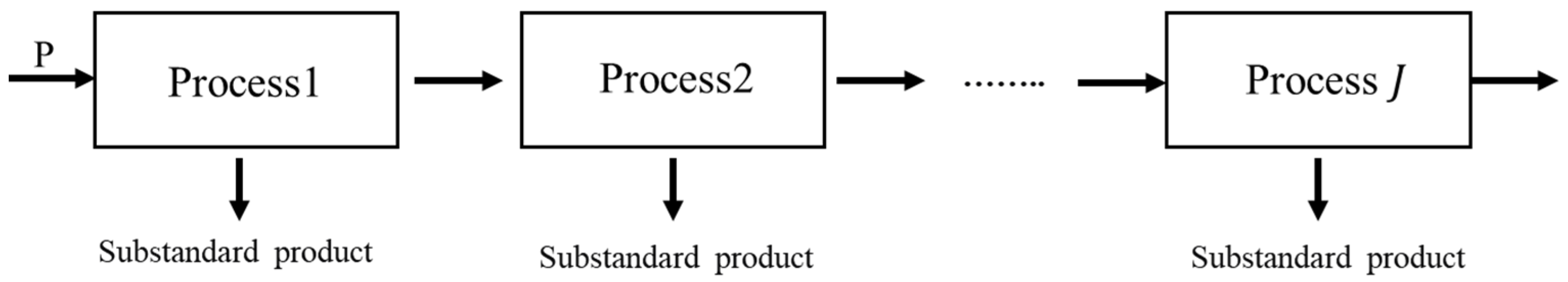
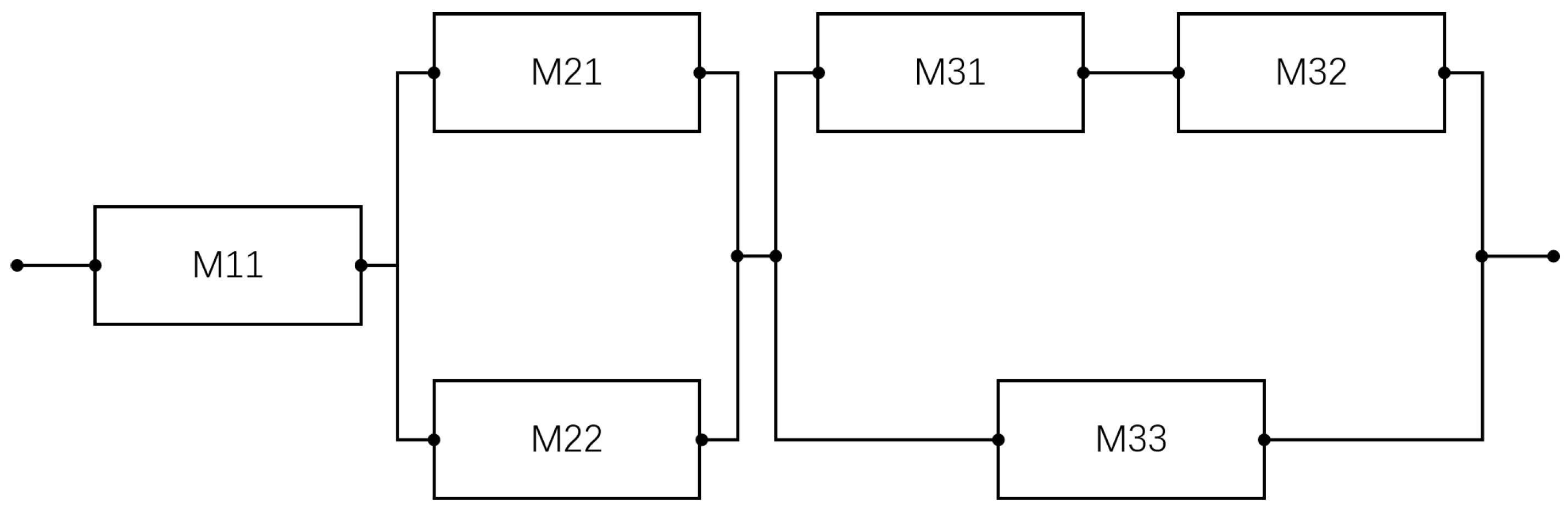
2.1. Leased Production System

The lessee rents equipment for the production of a specific type of product. The overall system comprises a leased production line consisting of J sequential processing stages, as shown in Figure 1. Each stage j ( j = 1 , 2 , ,   J ) is equipped with k j parallel-configured devices. For instance, within process j , one can find devices M j 1 , M j 2 , …, M j k j . The system supports both independent and coordinated operation modes. A disruption at any single processing stage results in the interruption of the entire production flow. All equipment is provided and maintained by the lessor, while the lessee pays rental fees based on usage. To improve maintenance efficiency and ensure uninterrupted production, both parties share real-time equipment condition data and collaborate in the optimization of maintenance strategies and decision-making processes.

2.1.1. Degradation Process of Critical Components

The machining quality of a product is closely tied to the condition of the equipment’s critical components, such as bearings and cutting tools. As these components progressively degrade, the precision and stability of the equipment decline, resulting in a gradual deterioration of product quality, including dimensional accuracy and surface finish. To describe the stochastic degradation process of these critical components, a Gamma process, characterized by non-negative and independent increments, is employed for modeling. Let X j k ( t ) denote the degradation level at time t , with X j k ( t ) 0 . The degradation increment over the time interval [ t 1 , t 2 ], denoted as ΔX = X j k ( t 2 ) X j k ( t 1 ) , is assumed to follow a Gamma distribution with shape parameter η j k ( t 2 t 1 ) and scale parameter θ j k . The probability density function is given as follows [28]:
f j k ( t 2 t 1 ) ( x ) = θ j k η j k ( t 2 t 1 ) x η j k [ ( t 2 t 1 ) 1 ] Γ [ η j k ( t 2 t 1 ) ] e θ j k x ,       x 0
At each processing stage, sensors continuously monitor leased equipment in real time, collecting data such as machining errors and vibration frequency. The defect rate of machine M j k is assumed to increase monotonically with its degradation level. This relationship is described by the following nonlinear expression [29]:
p ˜ j k ( t ) = p ˜ 0 + a [ 1 exp ( c X j k ( t ) b ) ]
where p ˜ 0 represents the initial defect rate when the system is in a brand-new state; a represents the boundary value for quality degradation; c and b are constants.

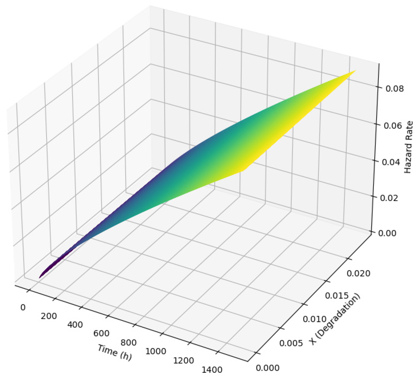
2.1.2. Proportional Hazards Model

The proportional hazards model (PHM) enables quantification of the influence of covariates on failure rates, thereby providing more accurate and reliable predictions. In this study, we consider a scenario involving a single covariate process, denoted by X = { X j k ( t ) : t 0 } , which represents the degradation process of a critical component. The PHM is expressed as the product of a baseline hazard function h 0 ( t ) and a covariate function g ( ) . The general form of the model is given as follows [30]:
h ( t X j k ( t ) ) = h 0 ( t ) g ( X j k ( t ) )
where h 0 ( t ) describes the effect of the inherent characteristics of the system (i.e., the baseline failure behavior), while g ( ) quantifies the influence of the covariate X j k ( t ) on the failure rate.

2.1.3. Overview of Maintenance Strategy

Maintenance activities are typically implemented using a single-machine PM strategy, where only the equipment that reaches a predefined maintenance threshold is serviced. However, this approach often leads to missed opportunities for system-level downtime optimization. To address this issue, this study proposes three types of maintenance actions. Based on the degradation state of the equipment, different maintenance strategies are selected. Let δ denote the maintenance effectiveness coefficient, reflecting the extent to which each maintenance action mitigates degradation. A hybrid failure rate model is employed to describe the impact of maintenance. By reasonably scheduling maintenance types and intervals, the goal is to achieve an optimal balance between maintenance effectiveness and cost.
Maintenance type M1: routine maintenance (RM). When the equipment’s failure rate has not yet reached the OM threshold D j k o m , RM is performed. This includes activities such as dust removal, lubrication, and tightening of components. The effectiveness of such maintenance is relatively low, but the cost is minimal, making it suitable for daily maintenance operations.
X j k M 1 ( t ) = ( 1 δ M 1 ) X j k ( t )
h M 1 ( t X j k ( t ) ) = h ( v n ( t ) X j k M 1 ( t ) )
Here, δ M 1 ( 0 , 1 ) represents the maintenance effectiveness of the RM activity.
Maintenance type M2: OM. This study proposes performing OM on leased equipment whose degradation level exceeds the OM threshold D j k o m , during either system-level downtime due to failure or scheduled periodic maintenance. OM is particularly suitable for complex equipment systems requiring multi-level maintenance at regular intervals. It is especially effective in resource-constrained environments where equipment performance has a direct impact on production efficiency. The improvement in equipment failure rate resulting from OM is described as follows:
X j k M 2 ( t ) = ( 1 δ M 2 ) X j k ( t )
h M 2 ( t X j k ( t ) ) = h ( v n ( t ) X j k M 2 ( t ) )
where δ M 2 ( 0 , 1 ) represents the maintenance effectiveness of the OM activity, and δ M 2 > δ M 1 .
Maintenance type M3: PM. When the equipment’s failure rate exceeds the PM threshold D j k p m , PM is performed. This activity partially restores the equipment’s condition and slows the rate of failure growth by reducing its virtual age. However, it does not restore the equipment to a like-new state. At this stage, the age reduction factor is relatively high, and the associated maintenance cost is also significantly greater.
X j k M 3 ( t ) = ( 1 δ M 3 ) X j k ( t )
h M 3 ( t X j k ( t ) ) = h ( v n ( t ) X j k M 3 ( t ) )
where δ M 3 ( 0 , 1 ) represents the maintenance effectiveness of the PM activity, and δ M 3 > δ M 2 .
In practical production operations, maintenance activities reduce the failure rate of leased equipment and improve its performance, but they cannot fully restore the equipment to a like-new condition. Therefore, at time t , the virtual age of the equipment is denoted by ν ( t ) , and it can be computed using the following equation [20]:
v ( t ) = t ( 1 ω Mi ) n τ
where n represents the maintenance interval and ω Mi ( i = 1 , 2 , 3 ) is the age reduction factor, reflecting the effect of different maintenance strategies on the degradation rate of the leased equipment.

2.1.4. Model Assumptions

To facilitate the development of the model, the following assumptions are made based on practical considerations:
(1)
The generation of defective products is solely determined by the condition of the equipment.
(2)
Maintenance activities do not introduce new failures; that is, after each maintenance action, the equipment is restored to a reasonable operational state through appropriate repair measures.
(3)
Compared to the duration of the lease period, maintenance time is negligible.
(4)
Corrective maintenance (CM) restores the equipment to operational status without altering its degradation level.
Several commonly adopted idealized assumptions are made in the modeling process of this study, including negligible maintenance duration, maintenance activities introducing no secondary failures, and CM not altering the equipment’s degradation state. These assumptions are widely used in the existing literature and help to ensure the mathematical tractability and analytical clarity of the model [17,31,32]. However, they may impose certain limitations in practical applications, as discussed below: (1) In real-world scenarios, particularly for complex or remotely deployed equipment, maintenance activities can consume significant time. The assumption of instantaneous maintenance may introduce biases in estimating system availability and customer waiting time, potentially underestimating the impact of maintenance-induced service interruptions in a leasing context. (2) In practice, maintenance actions may introduce new risks or fail to eliminate the original faults due to human errors, variations in spare part quality, or suboptimal repair strategies. Neglecting the possibility of secondary failures could lead to an overestimation of the reliability improvements resulting from maintenance interventions. (3) The assumption that corrective maintenance does not alter the degradation state overlooks the potential partial restoration or performance deterioration that may occur after emergency repairs. In some industrial settings, corrective actions taken under time constraints may compromise the remaining useful life of the equipment, thereby affecting its subsequent degradation trajectory.
Given these considerations, future research could enhance the current model by incorporating more realistic assumptions, such as randomly distributed maintenance durations and uncertainty in repair quality. These extensions would improve the model’s applicability to real-world leasing systems and enhance its predictive accuracy.

3. Optimization Modeling of Leasing Maintenance Strategy

3.1. Imperfect Maintenance Cost of the Lessor

The lessee utilizes the leased equipment to produce a certain product. During the lease period T L , all maintenance activities are performed by the lessor, who also bears the associated maintenance costs. Suppose the total number of maintenance actions during the lease term is N , then the maintenance cycle length is τ = T L / ( N + 1 ) ,   n = 1 , , N , where N is a positive integer.
The total cost C total ( t ) consists of the PM cost C PM and the CM cost C CM and is expressed as:
C total = C PM + C CM
where the maintenance cost C PM includes the cost of RM C M 1 , OM cost C M 2 , and PM cost C M 3 . The maintenance cost C PM is as follows:
C PM = C M 1 + C M 2 + C M 3

3.1.1. Maintenance Cost

The maintenance cost model uses a piecewise function to define the relationship between different levels of maintenance activities and their corresponding costs, expressed as follows:
c pm = { c j k M 1 if   h ( t X j k ( t ) ) < D j k o m , c j k M 2 if   D j k o m h ( t X j k ( t ) ) < D j k p m , c j k M 3 if   h ( t X j k ( t ) ) D j k p m .
The cost of RM is expressed as:
C M 1 = t = 1 T L j = 1 J k = 1 K c j k M 1 o j k ( t )
where o j k ( t ) is a binary variable indicating whether RM is performed on equipment at time t ( o j k ( t ) = 1 denotes performing RM on M j k , and o j k ( t ) = 0 denotes not performing RM), and c j k M 1 is the cost per RM action.
The cost of OM is expressed as:
C M 2 = t = 1 T L j = 1 J k = 1 K c j k M 2 u j k ( t )
where u j k ( t ) is a binary variable indicating whether OM is performed at time t ( u j k ( t ) = 1 denotes performing OM on M j k , and u j k ( t ) = 0 denotes not performing OM), and c j k M 2 is the cost per OM action.
The cost of PM is expressed as:
C M 3 = t = 1 T L j = 1 J k = 1 K c j k M 3 z j k ( t )
where z j k ( t ) is a binary variable indicating whether PM is performed at time t ( z j k ( t ) = 1 denotes performing PM on M j k , and z j k ( t ) = 0 denotes not performing PM), and c j k M 3 is the cost per PM action.

3.1.2. Failure and Penalty Costs

The CM cost C CM consists of two components: the penalty cost due to equipment failure and the cost of post-failure repair. The objective function is expressed as:
min C CM = min t = 1 T L { c P e n a l t y ( t ) + c R e p a i r ( t ) }
where c P e n a l t y ( t ) denotes the penalty cost at time t , and c R e p a i r ( t ) denotes the repair cost at time t .
Specifically, the total penalty cost at time t is:
c P e n a l t y ( t ) = j = 1 J k = 1 K s j k f j k ( t )
where s j k is the penalty coefficient, representing the fine imposed for equipment failure. f j k ( t ) is a binary variable indicating whether failure occurs at time t ( f j k ( t ) = 1 for failure, 0 otherwise).
Let m j k ( t ) be a binary variable indicating whether CM is performed at time t ( m j k ( t ) = 1 for repair, 0 otherwise). Then, the repair cost at time t is:
c R e p a i r ( t ) = j = 1 J k = 1 K c j k c m m j k ( t )
where c j k c m is the unit cost of corrective repair.

3.1.3. Leased Equipment Residual Value Model

The residual value B j k ( T L ) of leased equipment at the end of the lease term is influenced by its virtual age and maintenance history. To more accurately reflect the depreciation of value, the following age-based residual value model is used [21]:
B j k ( T L ) = B j k 0 1 v j k ( T L ) t j k
where B j k ( T L ) is the residual value of equipment M j k at the end of the lease term. B j k 0 is the initial residual value of equipment M j k . v j k ( T L ) is the virtual age of equipment M j k at the end of the lease term. t j k (non-zero) is the initial virtual age of the equipment M j k .
Now, the net residual value, which is defined as the difference between the equipment’s residual value and the total maintenance cost during the lease period, can be obtained as follows:
Π ( τ , D j k o m , D j k p m ) = j = 1 J k = 1 K B j k ( T L ) C total
where C total represents the total cost incurred during the lease period, and is the net residual value at the end of the lease term.

3.2. Customer Cost Model

From the perspective of leasing system operations, the operational status of equipment has a direct impact on the lessee’s performance. During equipment usage, the lessee mainly faces two types of loss risks: the first is downtime loss caused by equipment failure, and the second is quality loss resulting from performance degradation. This section considers failure-induced downtime and quality degradation driven by equipment reliability and develops a cost model of the lessee’s losses.
During the operation of leased equipment, failures often lead to system shutdowns, causing production interruptions. The economic loss resulting from such equipment unavailability is referred to as downtime loss, which is expressed as:
Q 1 = n = 1 N d = 1 Λ ( τ n ) c d P t d
where c d is the unit cost of downtime loss, and t d is the downtime due to failures.
Given the existence of a quality propagation effect between production stages—i.e., defective products from earlier stages negatively affect the quality in subsequent ones—this model assumes that defective items are removed at each stage and do not proceed to the next, as illustrated in Figure 2.
Let P denotes the constant input rate of raw materials. Then, at the first processing stage, the product output rate is given as follows [33]:
p 1 ( t ) = P [ 1 h 1 P ˜ 1 ( t ) T ]
The specific reasoning process is as follows:
p 1 ( t ) = P [ p 11 p ˜ 11 ( t ) + p 12 p ˜ 12 ( t ) + + p 1 K p ˜ 1 K ( t ) ] = P { 1 [ p 11 P p ˜ 11 ( t ) + p 12 P p ˜ 12 ( t ) + + p 1 K P p ˜ 1 K ( t ) ] } = P { 1 [ h 11 p ˜ 11 ( t ) + h 12 p ˜ 12 ( t ) + + h 1 K p ˜ 1 K ( t ) ] }
where h 1 = ( h 11 ,   h 12 ,   ,   h 1 K ) ,   h 1 k = p 1 k / P denotes the production capacity proportion of equipment M j k in the first processing stage, p ˜ j ( t ) = ( p ˜ j 1 ( t ) ,   p ˜ j 2 ( t ) ,   ,   p ˜ j K ( t ) represents the vector of quality degradation for all machines in stage j , as defined in Equation (2), and p ˜ j k ( t ) is the defective rate of M j k at time t .
Similarly, the output rate of the m th stage is as follows:
p m ( t ) = p m 1 ( t ) [ 1 h m P ˜ m ( t ) T ] = P j = 1 m [ 1 h j P ˜ j ( t ) T ]
The overall output rate of the system at time t is as follows:
p J ( t ) = P j = 1 J [ 1 h j P ˜ j ( t ) T ]
The defect rate of the entire production system at time τ n is given by:
r ( τ n ) = P p J ( τ n ) = P P j = 1 J [ 1 h j P ˜ j ( τ n ) T ] = P { 1 j = 1 J [ 1 h j P ˜ j ( τ n ) T ] }
where τ n denotes the starting time of the n th PM cycle.
Now, the quality-related losses can be obtained as follows:
Q 2 = n = 1 N c q r ( τ n )
where c q is the unit cost associated with quality loss caused by defective products. r ( τ n ) is the defect rate of the system at time τ n . The expected number of failures during the lease term, based on the PHM, is given as follows:
Λ ( τ n ) = τ n 1 τ n h ( t X j k ( t ) ) d t = τ n 1 τ n h 0 ( t ) g ( X j k ( t ) ) d t
The cost model of the lessee’s losses can be obtained as follows:
Q ( τ , D j k o m , D j k p m ) = Q 1 + Q 2 = n = 1 N d = 1 Λ ( τ n ) c d P t d + n = 1 N c q r ( τ n )

3.3. Cost Models for Both Parties in the Leasing System

For any optimization problem, the objective function plays a crucial role, as it defines the goal of the optimization and directly influences the solution [34]. In the leasing system, the primary objective of the lessor is to maximize the net residual value, while the lessee’s main objective is to minimize the total loss cost. The optimization problem is to solve the following non-linear, mixed-integer, and stochastic model:
max Π ( τ , D j k o m , D j k p m ) min Q ( τ , D j k o m , D j k p m ) s . t { τ :   n o n n e g a t i v e , D j k o m , D j k p m :   i n t e g e r , D j k o m D j k p m .
The maintenance decision-making process during the lease period is illustrated in Figure 3.

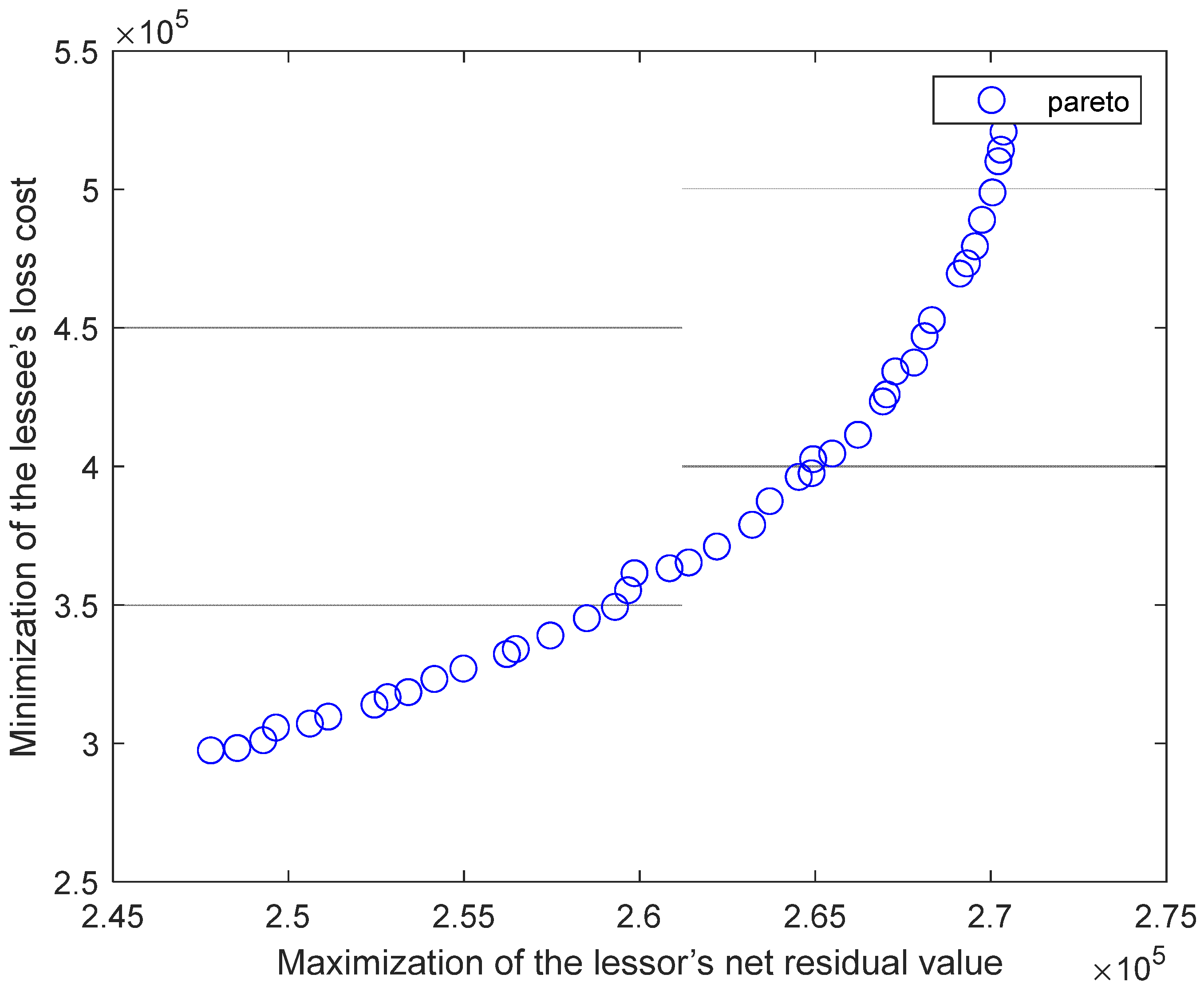
4. Experimentation and Analysis of the Results

4.1. Case Study

This section presents a case study to demonstrate and validate the proposed model. The case involves a machining center, where a company leases six pieces of equipment configured in a series–parallel system (as shown in Figure 4) to process cylindrical gear housings. These housings are used to connect the reducer and the differential, forming a key component in the reducer–differential assembly [35]. The specific task of the machining center is to bore holes for bearing seats. The quality of these holes, measured by their diameter and depth, is influenced by the degradation level of the boring cutter. Based on the system structure, there are four types of system-level downtime scenarios: ① Failure of M 11 ; ② Simultaneous failure of M 21 and M 22 ; ③ Simultaneous failure of M 31 and M 33 ; ④ Simultaneous failure of M 32 and M 33 . When the system experiences downtime due to these failures, CM can be performed, and OM can be considered taking this downtime opportunity.
In the case analysis of this study, we adopt the PHM to characterize the failure rate of the equipment in detail. The general form of the PHM is given in Equation (3). In practical applications, there are various forms of baseline hazard functions and link functions. However, the most commonly used is the Weibull PHM. This model consists of a Weibull-distributed baseline hazard function and an exponential link function. The baseline hazard function is defined as:
h 0 ( t ) = α j k β j k ( t β j k ) α j k 1
where α j k and β j k denote the shape and scale parameters of the Weibull distribution.
The specific formulation is as follows:
h ( t X j k ( t ) ) = α j k β j k ( t β j k ) α j k 1 exp ( γ j k X j k ( t ) )
where γ j k is the regression coefficient of the covariate.
Accordingly, the system’s reliability function is given by:
R j k ( t ) = Pr ( ξ > t X j k ( u ) , 0 < u < t ) = exp { 0 t α j k β j k ( t β j k ) α j k 1 exp [ γ j k X j k ( u ) ] d u }
where ξ represents the system’s lifetime at failure.
The values of model parameters are summarized in Table 1. The corresponding maintenance costs for the equipment are shown in Table 2 (All cost values in the table are expressed in USD). Additionally, the parameters are set as follows: p 0 = 0.004, a = 0.08, c = 0.005, b = 1.2. The production rate P is 400 units/day, the quality loss c q is 15 $/unit, and the downtime loss c d is 50 $/hour. The downtime duration t d ~ Exp ( 1.2 ) is measured in hours. The lease period T L is assumed to be 3 years. The age reduction factors are ω M 1 = 0.8, ω M 2 = 0.6, and ω M 3 = 0.4; the maintenance effect coefficients are σ M 1 = 0.2, σ M 2 = 0.4, and σ M 3 = 0.6.
Figure 5 presents a three-dimensional surface generated by substituting the parameters of equipment M 11 into the Weibull PHM, illustrating how the failure rate of the equipment varies with time and the degradation level of its core components. The x-axis represents time (in hours), the y-axis indicates the degradation level of core components (modeled using a Gamma process), and the z-axis denotes the failure rate (governed by the Weibull-based PHM, influenced jointly by time and degradation). From the figure, it is observed that in the early stages, the failure rate remains relatively low even as time progresses, provided the degradation level is low. However, once the degradation becomes significant, the failure rate escalates exponentially. This nonlinear relationship underscores the urgency of implementing proactive maintenance in the later stages of equipment health deterioration. The figure provides intuitive guidance for maintenance planning, enabling practitioners to identify “risk escalation inflection points” and optimize inspection frequency and intervention timing, thereby improving system availability.
The NSGA-II algorithm promotes the formation of the Pareto front by favoring non-dominated individuals and encouraging diversity among solutions [36]. The parameter settings are as follows: population size = 80, generations = 100, crossover probability = 0.8, mutation probability = 0.3. As shown in Figure 6, the Pareto-optimal solutions of the multi-objective optimization problem are displayed, with objectives being the maximization of the lessor’s net residual value and the minimization of the lessee’s loss cost. The x-axis represents the lessor’s net residual value (in USD), and the y-axis denotes the lessee’s loss cost (in USD). All values are normalized to enhance visualization. The Pareto front exhibits a typical nonlinear trade-off between the two objectives, reflecting how different maintenance strategies affect the interests of both parties. Solutions near the lower-right corner achieve both high residual value and low customer loss, representing ideal strategies. This figure serves as a decision-support tool for maintenance planning negotiations, helping companies balance economic returns and customer satisfaction. For instance, if the firm prioritizes customer retention, it may select solutions with lower loss costs; conversely, a focus on asset recovery may favor strategies that maximize equipment residual value.
Figure 7 and Figure 8 present the evolutionary curves of the lessor’s net residual value and the lessee’s loss cost over the course of the optimization, respectively. As seen in the figures, both objectives stabilize around the 40th generation, indicating that the NSGA-II algorithm exhibits good convergence and stability. This suggests that the model can produce consistent and repeatable outputs in practical deployment, contributing to the reliability of decision implementation. Furthermore, the evolution process can assist users in evaluating algorithm performance under different parameter settings, serving as a basis for future parameter tuning or sensitivity analysis.
To further address the multi-objective optimization problem, the entropy weight method (EWM) is employed to calculate the weights of each objective. First, both objectives are normalized, and a composite objective function is constructed using their weighted values. The resulting minimization form is expressed as:
Z = w 1 ( 1 Π Π min Π max Π min ) + w 2 Q Q min Q max Q min
where max and min denote the maximum and minimum net residual values, Q max and Q min represent the maximum and minimum loss costs, and w 1 and w 2 are the weights assigned to the net residual value and loss cost objectives, respectively, subject to the constraint w 1 + w 2 = 1 . When w 1 = 0.36 and w 2 = 0.64 , the overall objective function reaches its minimum, indicating that the loss objective (i.e., factors related to downtime and product quality) has a greater impact on the overall system performance. Under this condition, the maximum net residual value for the lessor is USD 270,362.00, and the minimum loss for the lessee is USD 297,499.59. The optimal PM cycle τ is 26 days. The OM thresholds D j k o m for the leased equipment are (0.324, 0.290, 0.259, 0.294, 0.300, 0.300), and the PM thresholds D j k o m are (0.534, 0.610, 0.600, 0.498, 0.503, 0.555). The maintenance costs incurred for each piece of equipment during the lease period are detailed in Table 3.
Table 4 provides detailed information to better illustrate the maintenance decision-making process. The values 1, 2, 3, and 4 represent RM, OM, PM, and CM activities, respectively.
Specifically, after the first two maintenance cycles, the failure rates of all devices remained below the OM thresholds, and RM was performed. After the third maintenance cycle, OM was performed on M 33 , while the other devices underwent RM. At the end of the 10th cycle, M 21 received RM, M 11 , M 22 , M 31 , and M 33 underwent OM, and M 32 received PM. After the 19th maintenance cycle, M 32 underwent PM, and the remaining devices received OM. Following the 20th cycle, M 21 , M 22 , M 32 , and M 33 underwent OM, while M 11 and M 31 underwent PM. An unexpected failure of M 11 occurred at the 30th maintenance cycle, resulting in system shutdown. At this point, other devices had reached their OM thresholds, so OM was performed, and CM was carried out on the failed device to restore system operation. Similarly, at the 38th maintenance cycle, another unexpected failure caused system downtime, during which OM was performed on other devices, and CM was executed on the failed device to resume operation.

4.2. Sensitivity Analysis

To evaluate the impact of key parameter variations on maintenance strategies and overall system performance, a sensitivity analysis was conducted on the lessor’s maintenance costs (including RM cost c j k M 1 , OM cost c j k M 2 , PM cost c j k M 3 , CM cost c j k c m , and penalty cost s j k ) and the lessee’s loss-related costs (downtime loss c d and quality loss c q ). Each parameter was varied within a range of ±25% and ±50%. The analysis focuses on the resulting changes in the maintenance cycle τ , OM thresholds D j k o m , PM thresholds D j k p m , the lessor’s net residual value , and the lessee’s loss cost Q , with weighted values ( w 1 , w 2 ) . The results are summarized in Table 5 below.
The analysis reveals that lessee-side costs, especially c d and c q , have a pronounced impact on maintenance frequency and lessee outcomes. Specifically, as c d increases, the optimal τ decreases and D j k o m are lowered, indicating that the system prioritizes frequent interventions to minimize service interruptions. On the lessor side, increases in c j k M 1 , c j k M 2 , and c j k M 3 result in longer maintenance cycles and higher thresholds, as the system reduces intervention frequency to contain direct maintenance expenditures. Among these, the c j k M 1 shows the highest sensitivity—raising c j k M 1 by 50% reduces by approximately 6.98%. This highlights the critical role of c j k M 2 in determining maintenance scheduling efficiency and economic returns for the lessor. Notably, shifts in s j k and c j k M 3 also affect both and τ , though to a lesser degree. The maintenance thresholds adapt accordingly to balance early or deferred maintenance decisions under different cost structures. Across all scenarios, the D j k o m consistently remain lower than the D j k p m , preserving the intended hierarchy of maintenance actions. Additionally, the weight distribution varies slightly with parameter changes, reflecting the model’s capability to dynamically adjust its optimization focus between lessor profit and lessee satisfaction under different economic priorities.
Overall, the I-OBAM strategy demonstrates stable performance across diverse cost environments, confirming its robustness and applicability in real-world rental scenarios with variable stakeholder cost structures.

4.3. Comparison of the Proposed Model with Two Other Conventional Models

To comprehensively evaluate the effectiveness of the proposed I-OBAM strategy, this study conducts a systematic comparison with two traditional maintenance strategies under the same leasing parameters and equipment reliability characteristics. The first is the streamlined reactive-level preventive maintenance (S-RLPM) strategy, which triggers routine or preventive maintenance based on the health status of individual equipment and predefined maintenance thresholds D j k p m . However, it does not take advantage of system-level downtime windows for coordinated interventions, which may lead to inefficient use of maintenance resources and scattered intervention timing. The corresponding maintenance cost is expressed as follows:
C S R L P M = n = 1 N ( c j k M 1 I { h ( t X j k ( t ) ) < D j k p m } + c j k M 3 I { h ( t X j k ( t ) ) > D j k p m } + c j k c m m j k ( t ) + s j k f j k ( t ) )
where N is the total number of maintenance actions during the lease term; c j k M 1 is the RM cost; c j k M 3 is the PM cost; c j k c m is the CM cost; s j k is the penalty cost; D j k p m is the PM thresholds; and I (A) is an indicator function that equals 1 if event A occurs and 0 otherwise.
The second strategy is the focused preventive risk-based maintenance (F-PRPM) strategy, where maintenance actions are triggered only when the device failure rate exceeds a predefined risk threshold. This strategy does not incorporate the OM mechanism, nor does it account for RM. It is more suitable for rental scenarios with relatively simple system structures or lower fault-tolerance requirements. The maintenance cost function is expressed as follows:
C F P R P M = n = 1 N ( c j k M 3 I { h ( t X j k ( t ) ) > D j k p m } + c j k c m m j k ( t ) + s j k f j k ( t ) )
To more intuitively illustrate the structural and operational differences between the proposed I-OBAM strategy and the two conventional benchmark strategies (S-RLPM and F-PRPM), the core characteristics of the three approaches are summarized in Table 6.
These two strategies are compared with the I-OBAM strategy, and the results are shown in Table 7.
(1) S-RLPM: Under this strategy, each leased device follows optimized preventive maintenance thresholds to determine whether to undergo routine or preventive maintenance. However, it does not consider maintenance opportunities arising from system-level downtime. Although the net residual value is slightly higher than that under the I-OBAM strategy, the significantly increased loss cost leads to a higher overall cost. Compared with the F-PRPM strategy, the S-RLPM demonstrates a slight advantage in improving the equipment condition, resulting in a marginally higher residual value.
(2) F-PRPM: This strategy only triggers preventive maintenance when the device failure rate exceeds the predefined threshold. Due to the high cost of preventive maintenance and lack of system-level optimization, it performs poorly. Since the F-PRPM does not incorporate system-level considerations and only reacts to high failure rates, it yields a slightly higher residual value but incurs greater loss costs. While its residual value and loss cost are similar to those of the S-RLPM, the absence of RM results in less effective cost optimization.
The above cost comparison indicates that the I-OBAM strategy exhibits significant advantages in jointly considering the growth characteristics of equipment failure rates and system-level maintenance optimization. First, by balancing routine and OM, the strategy effectively reconciles system reliability and maintenance costs, achieving better economic outcomes. Second, it accounts for environmental factors and inter-device dependencies, thus avoiding the local optimization limitations found in traditional strategies. Finally, by utilizing maintenance windows during system-wide downtime, it avoids redundant maintenance and resource waste. Moreover, the I-OBAM strategy recognizes the impact of regular light maintenance on equipment, ensuring system reliability while optimizing the allocation of maintenance resources, thereby attaining higher economic efficiency at a relatively low cost.

5. Conclusions

This study focuses on optimizing maintenance strategies for leased production equipment operating within series–parallel systems. The PHM is employed to characterize the failure rate evolution of equipment, thereby supporting condition-based maintenance decisions. For the lessor, a net residual value evaluation model is developed, accounting for the effects of virtual age and maintenance actions. For the lessee, a customer loss cost model is constructed based on quality loss and downtime. Within a multi-objective optimization framework, the NSGA-II algorithm is applied to obtain the Pareto optimal solution set, and the EWM is used to determine the relative importance of each objective. Experimental results demonstrate that the proposed strategy offers strong flexibility and adaptability, providing effective decision support for real-world leasing systems.
Despite offering a novel perspective on maintenance decision-making for multi-equipment leasing systems, the proposed model still requires improvements in dynamic responsiveness and generalizability when applied to more complex production environments and fluctuating market demands. For instance, the assumption that maintenance is instantaneous and fully effective may limit the model’s applicability in realistic scenarios. Moreover, the model does not explicitly incorporate lessee behavioral feedback (such as overuse or breach of contract), the impact of market volatility, or nonlinear depreciation processes, all of which may reduce its practical relevance. Notably, although sustainability is introduced as a key motivation for this research, the current model does not explicitly include environmental indicators such as carbon emissions or energy consumption. Future research can therefore extend this work in several directions: incorporating stochastic maintenance outcomes and delay factors to enhance realism; modeling contractual variations and customer behavioral responses to improve the representation of actual leasing dynamics; developing more representative residual value functions based on real-time market data and depreciation curves; and integrating environmental objectives into the optimization framework to better support sustainable leasing practices. Additionally, to promote industrial implementation, efforts should be made to enhance the model’s scalability and to develop real-time dynamic optimization algorithms that support high-quality development in the equipment leasing industry.

Author Contributions

Conceptualization and writing—original draft preparation, B.D.; software and resources, S.S.; supervision and writing—review and editing, G.C.; formal analysis, Y.W. All authors have read and agreed to the published version of the manuscript.

Funding

This research was funded by the National Natural Science Foundation of China (Grant No. 52371282).

Data Availability Statement

The data are contained within the article.

Conflicts of Interest

The authors declare no conflicts of interest.

References

  1. Wireman, T. Benchmarking Best Practices for Maintenance, Reliability and Asset Management; Industrial Press: Norwalk, CT, USA, 2014. [Google Scholar]
  2. Liu, B.; Shi, Y.; Yang, H. Optimal production and carbon reduction investment decision for manufacturers with leasing–selling strategies considering financing. Int. Trans. Oper. Res. 2025, 32, 3168–3196. [Google Scholar] [CrossRef]
  3. Tseng, M.-L.; Tan, R.R.; Chiu, A.S.; Chien, C.-F.; Kuo, T.C. Circular economy meets industry 4.0: Can big data drive industrial symbiosis? Resour. Conserv. Recycl. 2018, 131, 146–147. [Google Scholar] [CrossRef]
  4. Liu, B.; Wang, Y.; Yang, H.; Segerstedt, A.; Zhang, L. Maintenance service strategy for leased equipment: Integrating lessor-preventive maintenance and lessee-careful protection efforts. Comput. Ind. Eng. 2021, 156, 107257. [Google Scholar] [CrossRef]
  5. Li, K.; Yu, J. Leasing as a mitigation of financial accelerator effects. Rev. Financ. 2023, 27, 2015–2056. [Google Scholar] [CrossRef]
  6. Tukker, A. Product services for a resource-efficient and circular economy–a review. J. Clean. Prod. 2015, 97, 76–91. [Google Scholar] [CrossRef]
  7. Cook, M. Fluid transitions to more sustainable product service systems. Environ. Innov. Soc. Transit. 2014, 12, 1–13. [Google Scholar] [CrossRef]
  8. Tlili, L.; Anis, C.; Bouazizi, M. Optimal preventive maintenance policy for leased equipment for free with minimum quantity of consumables purchasing commitment by the lessee. J. Qual. Maint. Eng. 2023, 29, 708–725. [Google Scholar] [CrossRef]
  9. Wang, K.; Jing, H.; Wang, D.-D.; Jiang, F. Joint quality and maintenance decisions under servitization business model. Int. J. Prod. Res. 2024, 62, 1567–1585. [Google Scholar] [CrossRef]
  10. Ben Mabrouk, A.; Chelbi, A. Optimal maintenance policy for equipment leased with base and extended warranty. Int. J. Prod. Res. 2023, 61, 898–909. [Google Scholar] [CrossRef]
  11. Liu, B.; Pang, J.; Yang, H.; Zhao, Y. Optimal condition-based maintenance policy for leased equipment considering hybrid preventive maintenance and periodic inspection. Reliab. Eng. Syst. Saf. 2024, 242, 109724. [Google Scholar] [CrossRef]
  12. Zhang, Y.; Zhang, X.; Zeng, J.; Wang, J.; Xue, S. Lessees’ satisfaction and optimal condition-based maintenance policy for leased system. Reliab. Eng. Syst. Saf. 2019, 191, 106532. [Google Scholar] [CrossRef]
  13. Cao, Y.; Lu, C.; Dong, W. Importance measures for multi-state systems with multiple components under hierarchical dependences. Reliab. Eng. Syst. Saf. 2024, 248, 110142. [Google Scholar] [CrossRef]
  14. Chen, R.; Wang, S.; Zhang, C.; Dui, H.; Zhang, Y.; Zhang, Y.; Li, Y. Component uncertainty importance measure in complex multi-state system considering epistemic uncertainties. Chin. J. Aeronaut. 2024, 37, 31–54. [Google Scholar] [CrossRef]
  15. Cheng, G.; Shen, J.; Wang, F.; Li, L.; Yang, N. Optimal mission abort policy for a multi-component system with failure interaction. Reliab. Eng. Syst. Saf. 2024, 242, 109791. [Google Scholar] [CrossRef]
  16. Zhao, H.; Xu, F.; Liang, B.; Zhang, J.; Song, P. A condition-based opportunistic maintenance strategy for multi-component system. Struct. Health Monit. 2019, 18, 270–283. [Google Scholar] [CrossRef]
  17. Zheng, J.; Yang, H.; Wu, Q.; Wang, Z. A two-stage integrating optimization of production scheduling, maintenance and quality. Proc. Inst. Mech. Eng. Part B J. Eng. Manuf. 2020, 234, 1448–1459. [Google Scholar] [CrossRef]
  18. Ben Mabrouk, A.; Chelbi, A. Joint preventive maintenance and extended warranty strategy for leased unreliable equipment submitted to imperfect repair at failure. IFAC-Pap. 2022, 55, 1201–1206. [Google Scholar] [CrossRef]
  19. Xia, T.; Sun, B.; Chen, Z.; Pan, E.; Wang, H.; Xi, L. Opportunistic maintenance policy integrating leasing profit and capacity balancing for serial-parallel leased systems. Reliab. Eng. Syst. Saf. 2021, 205, 107233. [Google Scholar] [CrossRef]
  20. Liu, Y.; Liu, B.; Yang, H. Optimal pricing and financing strategies for leased equipment considering maintenance and lessees’ options. Int. J. Prod. Econ. 2024, 269, 109157. [Google Scholar] [CrossRef]
  21. Milošević, I.; Petronijević, P.; Arizanović, D. Determination of residual value of construction machinery based on machine age. Građevinar 2020, 72, 45–55. [Google Scholar]
  22. Chang, W.L.; Lo, H.-C. Joint determination of lease period and preventive maintenance policy for leased equipment with residual value. Comput. Ind. Eng. 2011, 61, 489–496. [Google Scholar] [CrossRef]
  23. Cao, Y.; Wang, P.; Xv, W.; Dong, W. Joint optimization of quality-based multi-level maintenance and buffer stock within multi-specification and small-batch production. Front. Eng. Manag. 2025, 1–20. [Google Scholar] [CrossRef]
  24. Zuo, W.; Fan, Y.; Xu, X.; Jiang, A. Grouping-maintenance of multi-components production system under ecological background. J. Ind. Eng. Manag. 2024, 17, 664–680. [Google Scholar] [CrossRef]
  25. Zhu, Z.; Xiang, Y.; Zeng, B. Multicomponent maintenance optimization: A stochastic programming approach. Inf. J. Comput. 2021, 33, 898–914. [Google Scholar] [CrossRef]
  26. Ruiz-Hernández, D.; Pinar-Pérez, J.M.; Delgado-Gómez, D. Multi-machine preventive maintenance scheduling with imperfect interventions: A restless bandit approach. Comput. Oper. Res. 2020, 119, 104927. [Google Scholar] [CrossRef]
  27. Vu, H.C.; Do, P.; Fouladirad, M.; Grall, A. Dynamic opportunistic maintenance planning for multi-component redundant systems with various types of opportunities. Reliab. Eng. Syst. Saf. 2020, 198, 106854. [Google Scholar] [CrossRef]
  28. Abdel-Hameed, M. A gamma wear process. IEEE Trans. Reliab. 1975, 24, 152–153. [Google Scholar] [CrossRef]
  29. Ben Mabrouk, A.; Chelbi, A.; Radhoui, M. Optimal imperfect maintenance strategy for leased equipment. Int. J. Prod. Econ. 2016, 178, 57–64. [Google Scholar] [CrossRef]
  30. Cox, D.R. Regression models and life-tables. J. R. Stat. Soc. Ser. B (Methodol.) 1972, 34, 187–202. [Google Scholar] [CrossRef]
  31. Cheng, G.Q.; Zhou, B.H.; Li, L. Integrated production, quality control and condition-based maintenance for imperfect production systems. Reliab. Eng. Syst. Saf. 2018, 175, 251–264. [Google Scholar] [CrossRef]
  32. Huang, Y.-S.; Ho, J.-W.; Hung, J.-W.; Tseng, T.-L. A customized warranty model by considering multi-usage levels for the leasing industry. Reliab. Eng. Syst. Saf. 2021, 215, 107769. [Google Scholar] [CrossRef]
  33. Cheng, G.; Li, L. Joint optimization of production, quality control and maintenance for serial-parallel multistage production systems. Reliab. Eng. Syst. Saf. 2020, 204, 107146. [Google Scholar] [CrossRef]
  34. Wickramasinghe, A.; Vilathgamuwa, M.; Nourbakhsh, G.; Corry, P. A Review of Dynamic Operating Envelopes: Computation, Applications and Challenges. Modelling 2025, 6, 29. [Google Scholar] [CrossRef]
  35. Lu, B.; Zhou, X. Opportunistic preventive maintenance scheduling for serial-parallel multistage manufacturing systems with multiple streams of deterioration. Reliab. Eng. Syst. Saf. 2017, 168, 116–127. [Google Scholar] [CrossRef]
  36. West, W.; Goupee, A.; Hallowell, S.; Viselli, A. Development of a Multi-Objective Optimization Tool for Screening Designs of Taut Synthetic Mooring Systems to Minimize Mooring Component Cost and Footprint. Modelling 2021, 2, 728–752. [Google Scholar] [CrossRef]
Figure 1. Multi-process leased production system.
Modelling 06 00052 g001
Figure 2. Quality degradation diagram.
Modelling 06 00052 g002
Figure 3. Maintenance decision flowchart.
Modelling 06 00052 g003
Figure 4. Leasing system structure.
Modelling 06 00052 g004
Figure 5. Failure rate variation with two factors graph.
Modelling 06 00052 g005
Figure 6. Pareto optimal solutions for multi-objective problem.
Modelling 06 00052 g006
Figure 7. Lessor’s objective optimization process.
Modelling 06 00052 g007
Figure 8. Lessee’s objective optimization process.
Modelling 06 00052 g008
Table 1. Equipment-related parameters.
α j k β j k η j k θ j k γ j k
M 11 1.81138.20.0132.960.0336
M 21 2.28234.60.2572.350.0216
M 22 2.16204.60.1733.430.0241
M 31 1.17142.10.4171.860.0152
M 32 1.56154.30.3253.230.0217
M 33 2.18254.60.2072.150.0306
Table 2. Related maintenance costs.
B j k 0 t j k c j k M 1 c j k M 2 c j k M 3 c j k c m s j k
M 11 100,00072242003105001000120
M 21 120,0006000220350400120070
M 22 130,0005544280340410121070
M 31 160,0003024160310420122060
M 32 110,00010,800140320310111060
M 33 100,0006600180210410101080
Table 3. Maintenance cost details.
RM CostOM CostPM CostCM Cost
M 11 3000155055005000
M 21 4400420000
M 22 4760217012000
M 31 800510000
M 32 1400288068200
M 33 1980336001010
Table 4. Partial decision-making process.
1231019203038
M 11 11122342
M 21 11112222
M 22 11122222
M 31 11122322
M 32 11133222
M 33 11222224
Table 5. Sensitivity analysis of system parameters.
ParametersVariation Range τ D j k o m D j k p m Q ( w 1 , w 2 )
-Basic case26(0.324, 0.29, 0.259, 0.294, 0.3, 0.3)(0.534, 0.61, 0.6, 0.498, 0.503, 0.555)270,362.00297,499.59(0.36, 0.64)
c j k M 1 −50%25(0.324, 0.312, 0.244, 0.309, 0.272, 0.283)(0.558, 0.515, 0.43, 0.497, 0.475, 0.448)284,726.26297,418.7(0.21, 0.79)
−25%23(0.332, 0.304, 0.269, 0.292, 0.3, 0.32)(0.547, 0.523, 0.481, 0.485, 0.482, 0.487)277,222.67293,226.43(0.28, 0.72)
+25%27(0.314, 0.292, 0.254, 0.299, 0.291, 0.305)(0.529, 0.515, 0.45, 0.532, 0.509, 0.52)263,831.90300,082.93(0.47, 0.53)
+50%29(0.333, 0.282, 0.275, 0.297, 0.298, 0.297)(0.553, 0.47, 0.446, 0.464, 0.468, 0.468)251,487.78295,633.28(0.22, 0.78)
c j k M 2 −50%23(0.324, 0.286, 0.267, 0.285, 0.308, 0.291)(0.566, 0.496, 0.484, 0.521, 0.485, 0.478)284,037.09285,734.19(0.22, 0.78)
−25%26(0.331, 0.299, 0.244, 0.304, 0.312, 0.308)(0.518, 0.514, 0.452, 0.514, 0.579, 0.536)272,973.42295,680.75(0.37, 0.63)
+25%28(0.33, 0.302, 0.255, 0.298, 0.298, 0.301)(0.543, 0.488, 0.462, 0.541, 0.489, 0.498)266,501.74290,989.52(0.49, 0.51)
+50%23(0.339, 0.294, 0.253, 0.277, 0.312, 0.318)(0.509, 0.469, 0.446, 0.471, 0.521, 0.472)261,948.23306,060.34(0.16, 0.84)
c j k M 3 −50%27(0.326, 0.291, 0.246, 0.284, 0.293, 0.288)(0.511, 0.527, 0.439, 0.484, 0.505, 0.509)279,190.44292,488.05(0.55, 0.45)
−25%23(0.331, 0.307, 0.256, 0.295, 0.297, 0.304)(0.534, 0.499, 0.454, 0.487, 0.524, 0.534)271,576.38310,204.82(0.54, 0.46)
+25%26(0.328, 0.287, 0.247, 0.299, 0.284, 0.3)(0.528, 0.495, 0.471, 0.485, 0.465, 0.481)266,885.17291,254.45(0.38, 0.62)
+50%27(0.333, 0.293, 0.27, 0.296, 0.299, 0.28)(0.589, 0.522, 0.466, 0.495, 0.492, 0.492)264,099.12287,070.96(0.57, 0.43)
c j k c m −50%26(0.321, 0.287, 0.257, 0.29, 0.295, 0.29)(0.523, 0.504, 0.465, 0.486, 0.528, 0.512)282,432.84288,921.15(0.34, 0.66)
−25%29(0.321, 0.291, 0.272, 0.295, 0.295, 0.302)(0.544, 0.481, 0.455, 0.495, 0.503, 0.488)275,080.84312,090.74(0.63, 0.37)
+25%23(0.311, 0.294, 0.256, 0.281, 0.29, 0.319)(0.481, 0.505, 0.456, 0.477, 0.491, 0.514)269,673.04302,211.79(0.38, 0.62)
+50%26(0.318, 0.293, 0.267, 0.294, 0.301, 0.283)(0.517, 0.473, 0.493, 0.473, 0.526, 0.517)261,344.01305,649.21(0.2, 0.8)
s j k −50%28(0.342, 0.3, 0.269, 0.298, 0.293, 0.301)(0.521, 0.508, 0.46, 0.52, 0.476, 0.506)282,656.92289,264.27(0.49, 0.51)
−25%25(0.316, 0.296, 0.261, 0.299, 0.307, 0.297)(0.492, 0.488, 0.45, 0.483, 0.512, 0.516)272,439.97294,761.94(0.71, 0.29)
+25%27(0.323, 0.277, 0.257, 0.295, 0.291, 0.316)(0.506, 0.443, 0.487, 0.503, 0.515, 0.511)265,870.04283,623.92(0.23, 0.77)
+50%24(0.325, 0.282, 0.259, 0.301, 0.288, 0.286)(0.534, 0.487, 0.455, 0.522, 0.502, 0.502)260,254.04308,731.47(0.48, 0.52)
c d −50%23(0.347, 0.273, 0.263, 0.273, 0.31, 0.308)(0.516, 0.455, 0.498, 0.464, 0.485, 0.501)276,322.51270,063.93(0.2, 0.8)
−25%25(0.326, 0.292, 0.248, 0.275, 0.3, 0.302)(0.534, 0.472, 0.474, 0.481, 0.463, 0.501)274,621.1285,059.54(0.13, 0.87)
+25%24(0.316, 0.288, 0.245, 0.29, 0.316, 0.291)(0.529, 0.495, 0.446, 0.431, 0.53, 0.505)279,944.42299,299.74(0.32, 0.68)
+50%23(0.317, 0.307, 0.247, 0.308, 0.282, 0.292)(0.519, 0.497, 0.448, 0.501, 0.491, 0.508)275,580.67302,928.61(0.12, 0.88)
c q −50%24(0.307, 0.287, 0.263, 0.293, 0.289, 0.289)(0.506, 0.513, 0.461, 0.503, 0.465, 0.527)261,154.58266,494.19(0.24, 0.76)
−25%28(0.329, 0.294, 0.256, 0.303, 0.307, 0.29)(0.533, 0.493, 0.463, 0.538, 0.522, 0.484)259,996.8276,709.62(0.61, 0.39)
+25%27(0.331, 0.31, 0.264, 0.282, 0.309, 0.318)(0.513, 0.498, 0.496, 0.499, 0.497, 0.489)282,357.61312,884.12(0.2, 0.8)
+50%24(0.317, 0.294, 0.281, 0.305, 0.303, 0.297)(0.49, 0.446, 0.481, 0.513, 0.501, 0.473)269,540.08328,939.72(0.35, 0.65)
Table 6. Structural and operational comparison.
Dimension/StrategyI-OBAMS-RLPMF-PRPM
Trigger mechanism D j k o m ,   D j k p m , with RM D j k p m , considers RM or PM D j k p m only, RM not considered
System-level opportunity maintenanceYes NoNo
Maintenance resource allocationDynamically scheduled using system downtime windowsIndependently scheduled per deviceReactive to individual device condition
Application suitabilityMulti-unit systems with high reliability and low lossSmall/medium-scale rentals focusing on operabilityRapid deployment with simplified logic
Table 7. Maintenance strategy comparison.
Strategy Q ( w 1 , w 2 )
I-OBAM270,362.00297,499.59(0.36, 0.64)
S-RLPM285,800.71397,802.77(0.34, 0.66)
F-PRPM271,798.65448,551.21(0.35, 0.65)
Disclaimer/Publisher’s Note: The statements, opinions and data contained in all publications are solely those of the individual author(s) and contributor(s) and not of MDPI and/or the editor(s). MDPI and/or the editor(s) disclaim responsibility for any injury to people or property resulting from any ideas, methods, instructions or products referred to in the content.

