A Novel Weak Fault Feature Extraction Method Based on Tensor Decomposition Model for Bearings

Abstract

The problem of extracting bearing weak fault features under variable-speed conditions with strong background noise interference remains challenging due to the limitations of existing feature extraction methods. These methods, especially those that rely on manual parameter tuning and rigid regularization, often struggle with noise suppression and robustness optimization, resulting in inaccurate extraction of weak fault features. To overcome this drawback, this study proposes a novel weak fault feature extraction method based on tensor decomposition model for bearings. First, the time–frequency tensor is constructed based on the short-time Fourier transform. Then, two types of fault properties in tensor are explored and an improved tensor decomposition model is proposed to realize the accurate extraction of weak fault features under variable-speed conditions. In addition, the decomposed feature tensor is conducted by a multichannel global energy-weighted fusion strategy, which significantly improves the robustness in extracting multichannel weak fault features. The effectiveness and superiority of the proposed method are systematically investigated through both simulated and experimental case studies. The results demonstrate that the method effectively eliminates background noise interference in measurements while augmenting the resolution of fault features.

1. Introduction

As the core supporting component of rotating machinery, the operational status of rolling bearings directly impacts equipment safety and reliability. Therefore, effective extraction of bearing fault characteristics is crucial for equipment health monitoring. In real industrial scenarios, bearings often operate under variable-speed conditions, leading to time-varying characteristics in fault frequency [1,2,3]. Meanwhile, bearing fault signals are frequently contaminated by strong background noise and interference from other components, posing significant challenges to feature extraction. Consequently, accurately extracting weak fault features from multichannel bearing measurement signals under variable-speed conditions with strong noise interference holds critical value for bearing fault diagnosis and equipment maintenance.

In recent years, time–frequency analysis techniques have provided new insights for variable-speed bearing fault diagnosis through joint time–frequency domain characterization [4]. As a powerful tool, time–frequency analysis simultaneously captures both temporal and spectral information of signals, enabling in-depth exploration of non-stationary signals’ time-varying characteristics and dynamic behaviors. A time–frequency representation (TFR) maps time-domain signals to the time–frequency plane via transformations such as short-time Fourier transform (STFT) [5] and wavelet transform (WT). These methods reveal fault features through energy distribution in the time–frequency plane. Among them, STFT treats non-stationary signals as a series of short-time stationary segments (achieved by applying sliding time windows) and performs Fourier transform on each segment to analyze the instantaneous spectrum at the window’s center time. It remains one of the most widely used time–frequency analysis methods. Compared to pure frequency-domain analysis, STFT exhibits unique advantages in fault detection under variable-speed conditions [6]. However, when the measured signal is contaminated by strong background noise, fault characteristics are easily obscured and become difficult to identify.

To effectively extract fault characteristic information from noisy environments, low-rank and sparse decomposition, as a feature extraction strategy, has been applied in multiple domains. Ma et al. [7] proposed a novel sparse low-rank matrix estimation method with nonconvex enhancement to extract the fault transients from observed noisy signal. Huang et al. [8] proposed an iteratively reweighted accurate sparse low-rank matrix estimation algorithm to further alleviate the problem of bias estimation and enhance the capabilities of the sparse low-rank method in effectively diagnosing bearing faults. However, the aforementioned methods are only applicable to bearings operating under constant-speed conditions. To address this limitation, Wang et al. employed a low-rank and sparse decomposition model to extract bearing fault characteristic components under variable-speed conditions [5,6]. Wang et al. employed a sparse low-rank algorithm to abstract the fault information from noisy signal interfered with by background noise and external interference [9,10]. Yu et al. proposed a new sparse time–frequency representation method to enhance TFA performance for bearing fault signals under variable-speed conditions [11]. However, the above fault diagnosis methods are limited to processing single-channel signals. With advancements in modern technology, the application of multi-sensor systems has simplified the acquisition of multichannel signals. By deploying multiple sensors at strategic locations on critical components, the collected multichannel signals can provide richer operational state information, significantly enhancing the accuracy and reliability of diagnostic results.

Tensors, as a natural and direct form of data representation for high-dimensional data, can maximize the preservation of data information and structure [12]. The structure correlation of multichannel signals and the fault modes has a certain mapping relationship, which can assist in the fault characteristics extraction from multichannel signals effectively. Based on this assumption, the multichannel processing method based on tensor decomposition has been widely researched in fault diagnosis. Yuan et al. [13] proposed a novel multichannel signals denoising method based on high order singular value decomposition. Ge et al. [14] studied tensor robust principal component analysis based on TSVD and achieved good applications in bearing faults diagnosis. This pioneering research demonstrates the feasibility of applying tensor low-rank and sparse estimation models in the field of fault diagnosis. However, most feature extraction methods based on tensor decomposition are based on constant-speed operating conditions, and are mostly based on the low-rank or sparsity of fault signals for tensor decomposition, which encounter challenges in extracting non-stationary fault features under strong background noise. To address the non-stationary characteristics and noise interference in multichannel variable-speed bearing signals, more improvements need to be proposed. On the one hand, how to characterize the time–frequency characteristics under variable-speed conditions in the tensor domain. On the other hand, how to explore the characteristics of multichannel fault signals to construct high-performance tensor decomposition models. In addition, how to improve the accuracy of fault signal extraction is also an urgent problem to be solved. Therefore, more improvements need to be proposed.

To address the non-stationary characteristics and noise interference in multichannel variable-speed bearing signals, this study proposes a fault feature extraction method for variable-speed rolling bearings via low-rank and sparse co-induced tensor singular space decomposition. The major contributions consist of the following three aspects:

(1)

In order to better display the multichannel signals under variable-speed conditions, the time–frequency tensor is constructed based on the short-time Fourier transform (STFT);

(2)

Two types of fault property in tensor are explored and an improved tensor decomposition model is proposed to realize the accurate extraction of weak fault features under variable-speed conditions;

(3)

The decomposed feature tensor is conducted by multichannel global energy-weighted fusion, which significantly improves the robustness in extracting multichannel weak fault features.

The remainder of this paper is arranged as follows. Section 2 introduces the tensor-related theory and tensor characterization method. The proposed method is described in Section 3. In Section 4, the effectiveness and superiority of the proposed method are validated through multichannel simulation signals. The superiority of the proposed method was verified through a laboratory typical fault simulation test in Section 5. Section 6 summarizes the main work and significance of this paper.

2. Methodology

2.1. Tensor Related Theory

Tensors are the high-dimensional extensions of vectors and matrices, symbolled as ($\mathcal{A},\mathcal{B},\mathcal{C}\cdots$) in this paper. Tensor singular value decomposition (TSVD) provides a simple and feasible mode decomposition approach for tensors [15]. For a third-order tensor $\mathcal{A}\in {ℝ}^{n_1\times n_2\times n_3}$, TSVD can decompose it into the form of tensor products by:

$$\mathcal{A}=\mathcal{U}\ast \mathcal{S}\ast {\mathcal{V}}^T$$

(1)

where $\mathcal{U}\in {ℝ}^{n_1\times n_1\times n_3}$, $\mathcal{V}\in {ℝ}^{n_2\times n_2\times n_3}$ are orthogonal tensor and $\mathcal{S}\in {ℝ}^{n_1\times n_2\times n_3}$ is a diagonal tensor as shown in Figure 1. TSVD can be computed efficiently via multiple matrix SVD in Fourier domain [16,17].

2.2. Tensor Construction of Multichannel Signals Based on Short-Time Fourier Transform

Under variable-speed operating conditions, the frequency of vibration signals exhibits continuous temporal variations, rendering the direct construction of a time-series attractor matrix inadequate for capturing these dynamic characteristics. Such an approach inherently overlooks the non-stationarity and localized variations of the signals, thereby rendering traditional signal processing methods designed for steady-state conditions inapplicable. As one of the most widely utilized time–frequency analysis techniques, the short-time Fourier transform (STFT) conceptualizes non-stationary processes as a superposition of multiple short-term stationary signals. By employing a windowing process to impart short-term stationarity and subsequently applying the Fourier transform to these segmented signals, STFT enables the analysis of the spectral content at the central moment, thereby effectively reflecting the temporal evolution of frequency components. Furthermore, by integrating tensors—the most direct and efficient representation of high-dimensional data—the high-order characterization of vibration signals based on STFT can comprehensively capture the time-varying characteristics of multichannel non-stationary signals. The time–frequency ridges within the time–frequency tensor, which encode fault-related features, provide a robust foundation for more comprehensive and detailed analytical insights.

STFT is an improvement based on the classical Fourier transform. For continuous time signals $s(t)$, the definition of STFT is as follows:

$${\mathrm{STFT}}_s(t,f)={{\displaystyle \int }}_{-\infty }^{+\infty }s(\tau ){\omega }^{\ast }(\tau -t)e^{-j2\pi f\tau }d\tau$$

(2)

where t and f represent time and frequency variables, respectively. $\omega (t)$ is a sliding window function, ${\omega }^{\ast }(t)$ is the conjugate of window function $\omega (t)$, and ${\mathrm{STFT}}_s(t,f)$ represents the spectral distribution of signal s at time t.

Based on the time–frequency transformation method mentioned above, we introduce a high-order tensor representation method based on STFT. Firstly, signals from multiple acceleration sensors at different positions and directions of the rotating equipment are collected. Then, STFT is used to convert the vibration signals of different channels from the time domain to the time–frequency domain, obtaining the time–frequency matrices of each channel. Finally, the time–frequency matrices of each channel are mapped into a forward slice of a tensor and arranged as tensors along the third-dimensional direction to obtain the time–frequency tensor $\mathcal{Z}\in {ℝ}^{N_1\times N_2\times N_3}$, where N₁, N₂, and N₃ are frequency, time, and channel number, respectively.

By exploring the spatial characteristics of fault features in the time–frequency tensor based on STFT, fault feature information can be effectively extracted from multi-source vibration signals of rolling bearings under variable-speed conditions.

3. Proposed Method

3.1. Exploration of Low-Rank and Sparsity Co-Induced Mechanism of Fault Features Within the Tensor

Under variable-speed operating conditions, the complex and dynamic operational states of rotating equipment render traditional fault diagnosis methods inadequate for effectively extracting signal characteristics. Therefore, conducting an in-depth investigation into the characteristic induction mechanisms of fault features embedded within time–frequency tensors, which are constructed from multichannel signals, is of paramount importance for effectively revealing latent fault information during the operational process. By analysing the time–frequency characteristics of multi-source signals under variable-speed conditions, we can capture variations in vibration patterns across different rotational speeds, which provides a robust foundation for the subsequent tensor singular space decomposition model. Consequently, this section will focus on a detailed exploration and elucidation of the characteristic mechanisms governing fault components within time–frequency tensors.

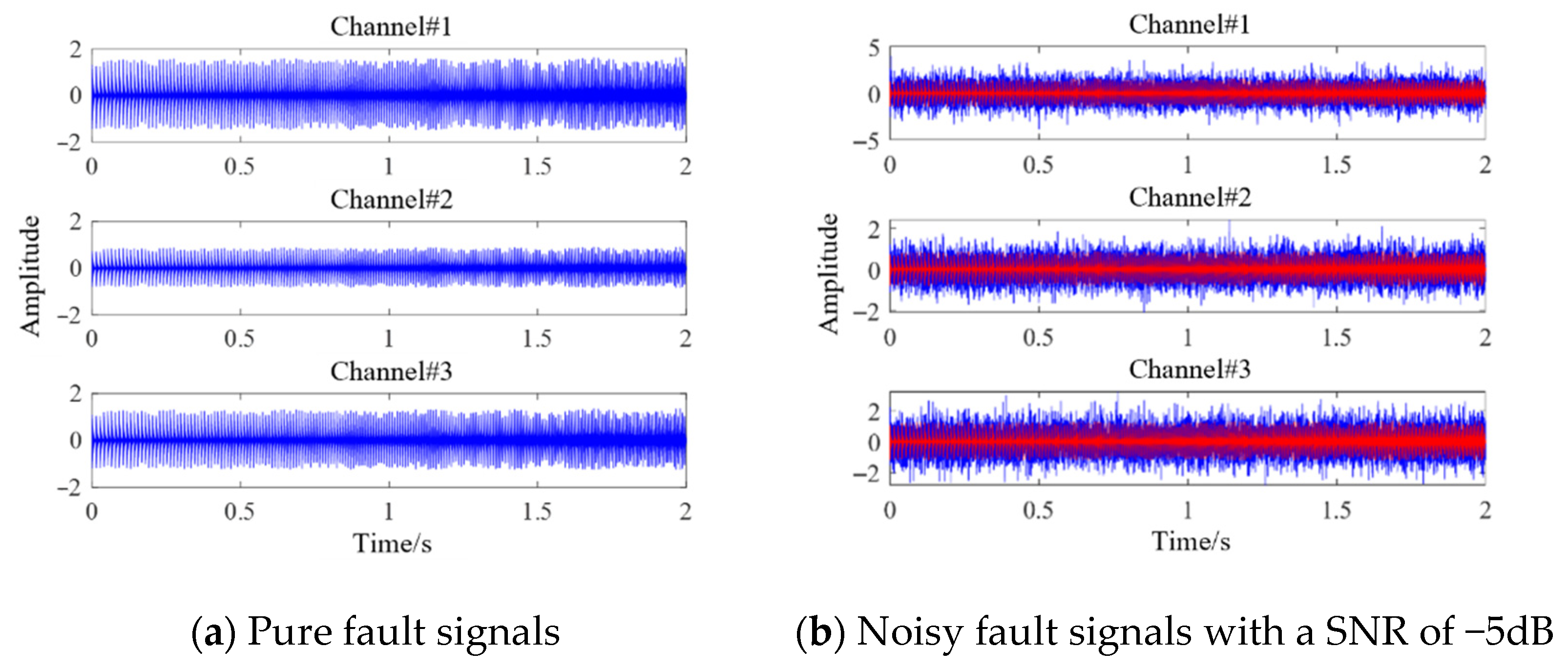
In this section, three time-domain signals of bearing outer race faults under variable-speed operating conditions are simulated to replicate the time-domain data collected by three channels in real-world scenarios. The detailed simulation parameters for the outer race fault signals will be thoroughly described in Section 4.1. The simulated pure fault time-domain signals are illustrated in Figure 2a. To simulate the variations in data collected by different sensors, the signal amplitudes for all three channels are randomly generated. In practical engineering applications, the collected fault signals are often accompanied by strong environmental noise and interference from other components. Therefore, Gaussian white noise with a signal-to-noise ratio (SNR) of -5dB is added to three outer race fault signals under the variable-speed conditions to replicate the complex acquisition environment. The simulated noisy fault time-domain signals are shown in Figure 2b, with the red portions representing the pure fault signals. From Figure 2, it is evident that the fault characteristics in the noisy signals are severely obscured by the noise and completely submerged under intense background interference.

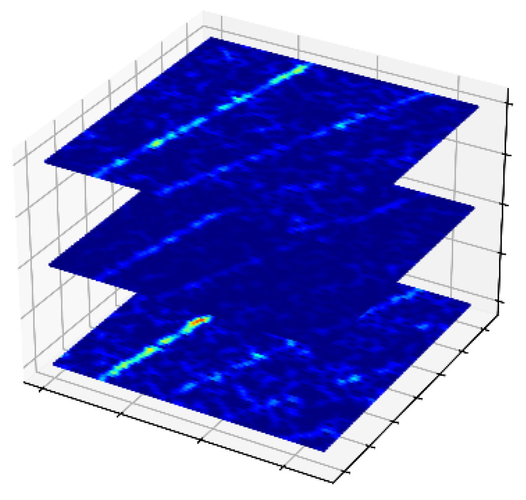
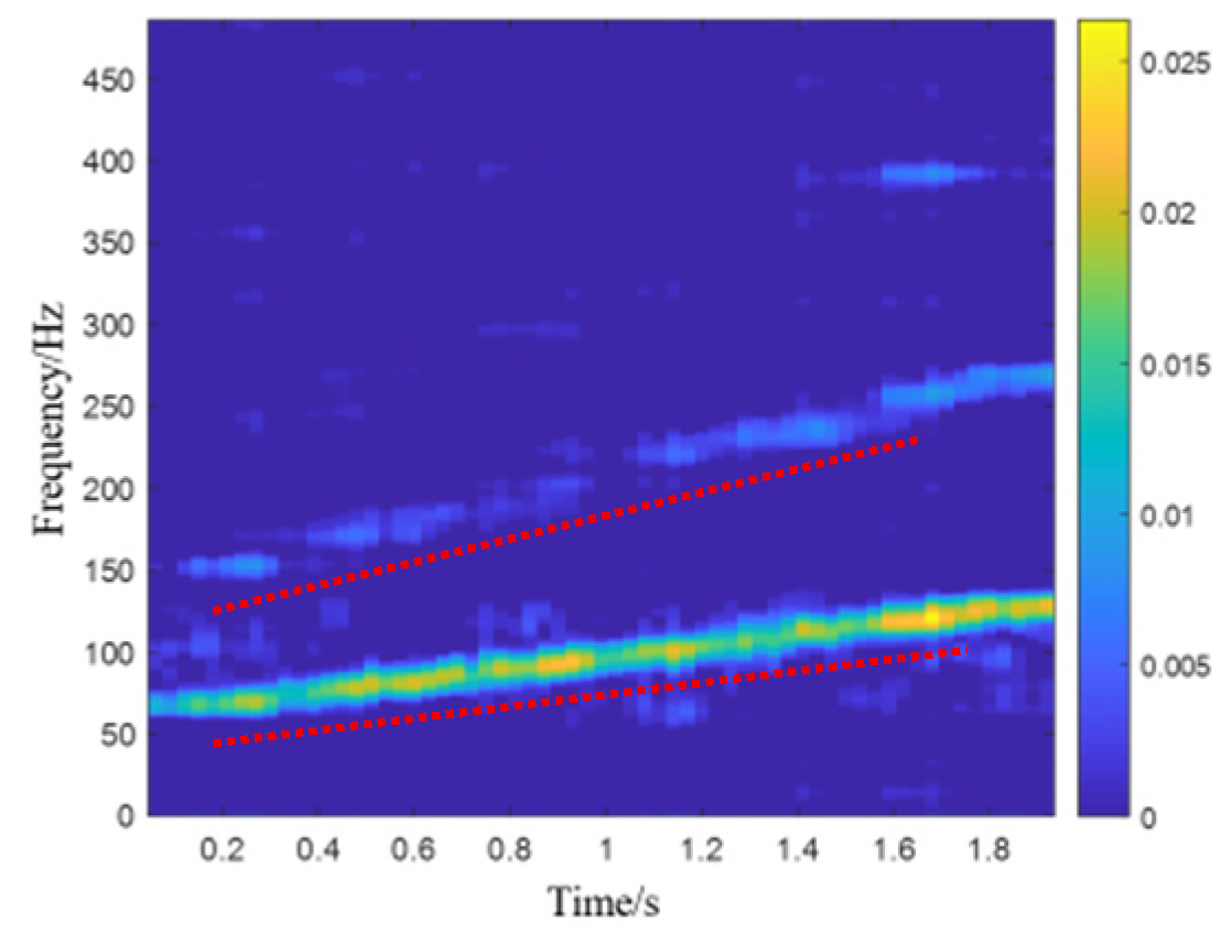
Based on the high-order tensor representation method of multichannel variable-speed signals in Section 2.2, STFT is used to calculate the time–frequency representation matrix of three pure fault signals collected from the same time range, as shown in Figure 3. Then, the time–frequency representation matrix obtained from each channel of data is used as a forward slice to form a third-order tensor $\mathcal{X}\in {ℝ}^{N_1\times N_2\times N_3}$, where N₁, N₂, and N₃ represent frequency, time, and channel number, respectively. The results are shown in Figure 4.

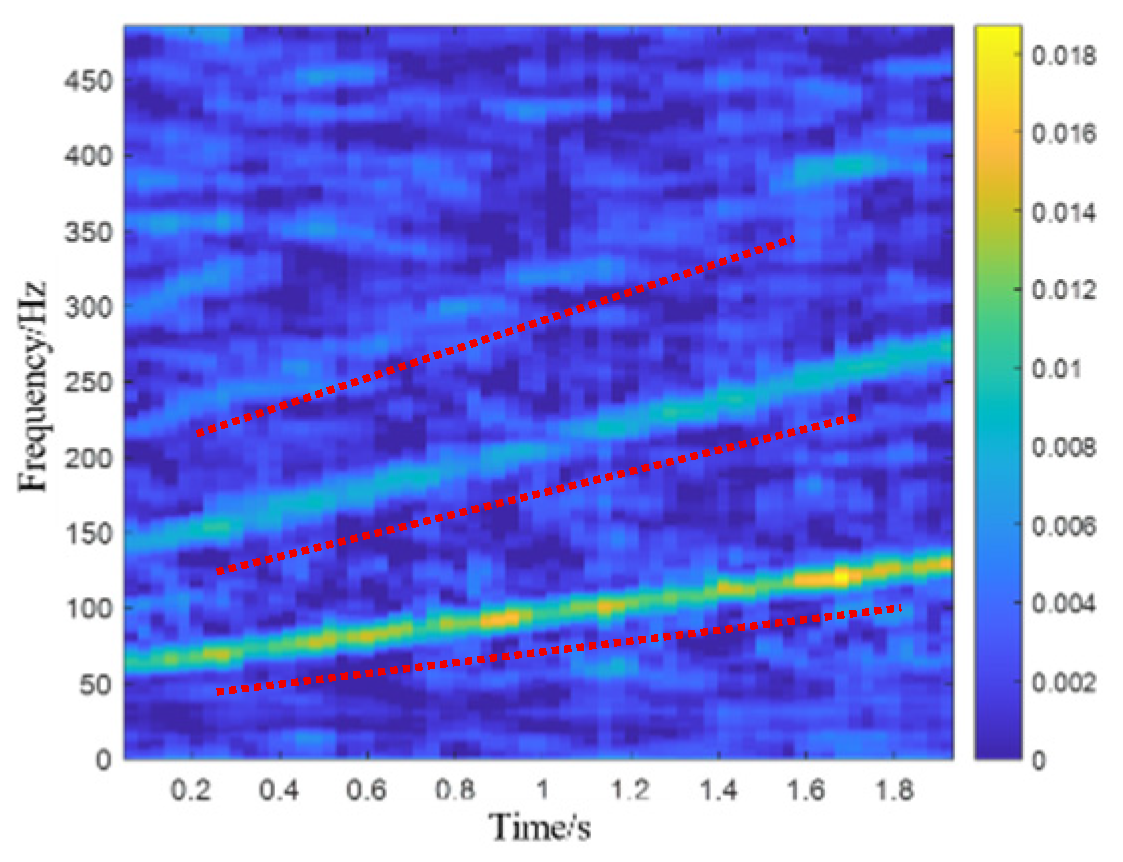
Meanwhile, we also performed time–frequency transformation and higher-order tensor characterization on the simulated noisy outer race fault signals, obtaining the corresponding time–frequency representation matrices and time–frequency tensors, as shown in Figure 5 and Figure 6.

From Figure 5 and Figure 6, it can be observed that the time–frequency ridges of the fault signals in the time–frequency tensor constructed from the noisy signals are severely contaminated by noise, making them difficult to be clearly identified. To better extract the fault features, it is necessary to conduct an in-depth exploration and analysis of the structural characteristics of the time–frequency tensor.

Based on the TSVD method mentioned in Section 2.1, the tensor constructed from the signals is processed. After decomposition, the singular values of the first frontal slice of the diagonal tensor can represent the tubal rank characteristics of the tensor. Therefore, we apply TSVD to the tensor constructed from the pure fault signals and arrange the singular values of the first slice in descending order, as shown in Figure 7. From Figure 7, it is evident that the first singular value dominates the distribution, indicating that the time–frequency representation tensor of the pure outer race fault exhibits strong low tubal rank characteristics.

At the same time, it is clearly visible from Figure 4 that in the time–frequency representation tensor, most of the tensor elements are zero, with significant values only appearing at the time–frequency ridges representing the fault features. Moreover, distinct peaks are observed at the same positions across different channels, demonstrating that the time–frequency tensor of the pure outer race fault possesses strong tubal sparsity characteristics.

However, the time–frequency representation tensor of noisy signals typically does not exhibit these two structural characteristics. To eliminate background noise interference, considering these two characteristics of fault features, this study proposes a low-rank sparse co-induced mechanism. The introduction of this mechanism lays the foundation for the subsequent tensor singular space decomposition model, thereby achieving effective separation of fault features from noise.

3.2. Tensor Singular Space Decomposition Model

Based on the two types of fault structural characteristics discovered in the time–frequency tensor under variable-speed in the previous section: low-rank and sparsity, we decide to use tensor low-rank and sparsity approximation method to extract fault features and separate them from the original signal.

The goal is to estimate a low-rank sparse tensor $\mathcal{X}$ from a noisy tensor $\mathcal{Y}$ , such as:

$$\mathcal{Y}=\mathcal{X}+\mathcal{W}$$

(3)

where $\mathcal{W}$ represents the additive Gaussian white noise tensor.

Based on the low-rank and sparsity co-induced mechanism mentioned above to estimate the fault tensor, we first propose the following optimization problem:

$$\arg \underset{\mathcal{X}\in {ℝ}^{N_1\times N_2\times N_3}}{\min }\left\{{\displaystyle \frac{1}{2}}\parallel \mathcal{Y}-\mathcal{X}{\parallel }_{ F}^2+{\lambda }_0\parallel \mathcal{X}{\parallel }_{ \ast }+{\lambda }_1\parallel \mathcal{X}{\parallel }_{ 1}\right\}$$

(4)

where $\parallel •{\parallel }_{ \ast }$ is the tensor nuclear norm, $\parallel •{\parallel }_{ 1}$ is the 1-norm, and ${\lambda }_{ \mathrm{i}}$ ≥ 0 is the regularization parameter. The tensor nuclear norm induces low-rank in tensor singular spaces, while the 1-norm induces sparsity of elements in tensors.

However, when the 1-norm is used as a sparsity inducing regularization, it fails to induce data with certain structural relationships. Therefore, the sparsity problem in the above formulation is generally considered too relaxed. Additionally, the performance of the tensor nuclear norm constrained by singular space low-rankness is suboptimal.

To more accurately estimate the non-zero signal values with specific structural relationships in the tensor, smoother constraints are preferred over the 1-norm. Furthermore, penalty functions with greater flexibility can induce low-rankness more effectively than tensor nuclear norm. Thus, this study proposes the following tensor singular space decomposition model:

$$\arg \underset{\mathcal{X}\in {ℝ}^{N_1\times N_2\times N_3}}{\min }\{{\displaystyle \frac{1}{2}}\parallel \mathcal{Y}-\mathcal{X}{\parallel }_{ F}^2+{\lambda }_0{\displaystyle \sum _{i=1}^{n_3}{\displaystyle \sum _{j=1}^n{f}_{\tau ,\gamma }({\sigma }_j^{(i)}(\mathcal{X}))}}+{\lambda }_1\parallel \mathcal{X}{\parallel }_{ 1,1,2}\}$$

(5)

where $f_{\tau ,\gamma }(\sigma )$ is the adaptive threshold function, $\parallel •{\parallel }_{ 1, 1, 2}$ is the 112-norm of the tensor. The adaptive threshold function is used to constrain the low-rank property of tensor singular values. The 112-norm constrains the sparsity of elements in the tensor. The adaptive threshold function is defined as follows:

$$f_{\tau ,\gamma }(\sigma )=\left\{\begin{array}{l}0\hspace{0.17em}\hspace{0.17em}\hspace{0.17em}\hspace{0.17em}\hspace{0.17em}\hspace{0.17em}\hspace{0.17em}\hspace{0.17em}\hspace{0.17em}\hspace{0.17em}\hspace{0.17em}\hspace{0.17em}\hspace{0.17em}\hspace{0.17em}\hspace{0.17em}\hspace{0.17em}\hspace{0.17em}\hspace{0.17em}\hspace{0.17em}\hspace{0.17em}\hspace{0.17em}\hspace{0.17em}\hspace{0.17em}\hspace{0.17em}\hspace{0.17em}\hspace{0.17em}\hspace{0.17em}\hspace{0.17em}\hspace{0.17em}\hspace{0.17em}\hspace{0.17em}\hspace{0.17em},\sigma \le \tau \\ \sigma ·\left(1-{({\displaystyle \frac{\tau }{\sigma }})}^{\gamma }\right) ,\sigma >\tau \end{array}\right.$$

(6)

where $\tau$ is the threshold, and $\gamma$ controls the shape of the inverse proportional function. More detailed information can be found in [18]. The new constraint sparsity 112-norm is proposed in the above equation, so the following mainly elaborates on the superiority of the 112-norm.

As mentioned above, the 1-norm as a penalty function for inducing sparsity is relatively lenient. The reason is that the 1-norm treats each element in the forward slice independently, without considering the correlation between fault features in multiple forward slices and cannot induce data with certain structural relationships. Therefore, we introduce the 112-norm of the tensor, defined as the sum of the 2-norm of all pipe vectors in a certain dimension of the tensor. Here, we take the third dimension as an example, as follows:

$$\parallel \mathcal{A}{\parallel }_{ 1,1,2}={\displaystyle \sum _{i_1}^{I_1}{\displaystyle \sum _{i_2}^{I_2}{‖\mathcal{A},(i_1,i_2,:)‖}_2}}$$

(7)

The 112-norm to some extent enhances the continuity and sparsity between multiple forward slices of the tensor, constraining the structural correlation between multiple channels.

This decomposition model introduces structured sparse norm constraints on fault features and combines adaptive threshold functions to achieve a dynamic balance of low-rank constraints, which can achieve good fault feature extraction results.

3.3. Algorithm Derivation

The alternating direction multiplier method (ADMM) algorithm will be used for aforementioned low-rank and sparsity co-induced tensor singular space decomposition model.

Firstly, an auxiliary variable $\mathcal{Z}$ is set to decompose the complex optimization problem into several simple sub-problems. Then, the optimization problem is transformed into the following equation:

$$\arg \underset{\mathcal{X}}{\min }\{{\displaystyle \frac{1}{2}}\parallel \mathcal{Y}-\mathcal{X}{\parallel }_{ F}^2+{\lambda }_0{\displaystyle \sum _{i=1}^{n_3}{\displaystyle \sum _{j=1}^n{f}_{\tau ,\gamma }({\sigma }_j^{(i)}(\mathcal{Z}))}}+{\lambda }_1\parallel \mathcal{X}{\parallel }_{ 1,1,2}\} \mathrm{s}.\mathrm{t}. \hspace{0.17em}\mathcal{X}=\mathcal{Z}$$

(8)

According to the ADMM, the above problem is transformed into the following three sub-problems, where $\mu$ is the penalty coefficient and $\mathcal{D}$ is the Lagrange multiplier:

$$\mathcal{X}=\arg \underset{\mathcal{X}}{\min }\{{\displaystyle \frac{1}{2}}\parallel \mathcal{Y}-\mathcal{X}{\parallel }_{ F}^2+{\displaystyle \frac{\mu }{2}}{‖\mathcal{X}-(\mathcal{Z}+\mathcal{D})‖}_{ F}^2+{\lambda }_1\parallel \mathcal{X}{\parallel }_{ 1,1,2}\}$$

(9)

$$\mathcal{Z}=\arg \underset{\mathcal{Z}}{\min }\{{\displaystyle \frac{\mu }{2}}{‖\mathcal{X}-(\mathcal{Z}+\mathcal{D})‖}_{ F}^2+{\lambda }_0{\displaystyle \sum _{i=1}^{n_3}{\displaystyle \sum _{j=1}^n{f}_{\tau ,\gamma }({\sigma }_j^{(i)}(\mathcal{Z}))}}\}$$

(10)

$$\mathcal{D}=\mathcal{D}-(\mathcal{X}-\mathcal{Z})$$

(11)

Combining the quadratic term and ignoring the constant term, sub-problem (9) can be rewritten as:

$$\mathcal{X}=\arg \underset{\mathcal{X}}{\min }\{{\displaystyle \frac{1}{2}}\parallel {\displaystyle \frac{1}{1+\mu }}(\mathcal{Y}+\mu (\mathcal{Z}+\mathcal{D}))-\mathcal{X}{\parallel }_{ F}^2+{\displaystyle \frac{{\lambda }_1}{1+\mu }}\parallel \mathcal{X}{\parallel }_{ 1,1,2}\}$$

(12)

There are four parameters that need to be determined in the proposed tensor singular space decomposition model, namely the parameters $\tau$ and $\gamma$ of the adaptive threshold function, and the regularization parameters ${\lambda }_0$ and ${\lambda }_1$ of the decomposition model. The selection method of adaptive threshold function parameters has been discussed in [18] and will not be elaborated on here. The regularization parameters that constrain the low-rank and sparsity of faults play a decisive role in the decomposition model. The selection of these two regularization parameters affects the proportion of the two characteristics of faults in the estimation model, directly affecting the extraction effect of fault features. Therefore, in this section, we need to determine the regularization parameters ${\lambda }_0$ and ${\lambda }_1$ (${\lambda }_i={\beta }_i\sigma$) of the decomposition model.

Therefore, the final optimization problem solving process is shown in Algorithm 1.

Algorithm 1. Solve low-rank and sparsity co-induced tensor singular space decomposition model by ADMM

Input: tensor $\mathcal{Y}\in {ℝ}^{N_1\times N_2\times N_3}$, parameters ${\lambda }_0,{\lambda }_1,\tau ,\gamma ,\mu ,\xi$, maximum iterations $k_{\max }$;

While convergence is not satisfied do

1. Update ${\mathcal{X}}_{k+1}$ by: ${\mathcal{X}}_{k+1}=\arg \underset{\mathcal{X}}{\min }{\displaystyle \frac{1}{2}}\parallel {\displaystyle \frac{1}{1+\mu }}(\mathcal{Y}+\mu ({\mathcal{Z}}_k+{\mathcal{D}}_k))-\mathcal{X}{\parallel }_{ F}^2+{\displaystyle \frac{{\lambda }_1}{1+\mu }}\parallel \mathcal{X}{\parallel }_{ 1,1,2}$;

2. Update ${\mathcal{Z}}_{k+1}$ by: ${\mathcal{Z}}_{k+1}=\arg \underset{\mathcal{Z}}{\min }{\displaystyle \frac{\mu }{2}}{‖{\mathcal{X}}_{k+1}-(\mathcal{Z}+{\mathcal{D}}_k)‖}_{ F}^2+{\lambda }_0{\displaystyle \sum _{i=1}^{n_3}{\displaystyle \sum _{j=1}^n{f}_{\tau ,\gamma }({\sigma }_j^{(i)}(\mathcal{Z}))}}$;

3. Update ${\mathcal{D}}_{k+1}$ by: ${\mathcal{D}}_{k+1}={\mathcal{D}}_k-({\mathcal{X}}_{k+1}-{\mathcal{Z}}_{k+1})$;

4. Check for convergence: ${‖{\mathcal{X}}_{k+1}-{\mathcal{X}}_k‖}_{\infty }\le \xi ,{‖{\mathcal{Z}}_{k+1}-{\mathcal{Z}}_k‖}_{\infty }\le \xi ,{‖{\mathcal{X}}_{k+1}-{\mathcal{Z}}_{k+1}‖}_{\infty }\le \xi$.

End

Output: $\mathcal{X}$

3.4. Global Energy Weighted Fusion Evaluation Strategy

The fault features $\mathcal{X}\in {ℝ}^{N_1\times N_2\times N_3}$ extracted by the above methods are still tensors. In order to better identify fault, this study proposes a time–frequency ridge energy weighted fusion evaluation strategy. By fusing the fault feature tensor along the channel direction, a fused time–frequency matrix is obtained. Considering that each channel contains different levels of fault information, this study proposes a global energy weighted fusion matrix. Taking three channels as an example, the global energy weighted fusion steps are as follows:

(1) Calculate the total energy of each channel:

$$E_i=\sum _{t,f}{\left|X_i(t,f)\right|}^2,(i=1,2,3)$$

(13)

(2) Calculate normalized weights:

$$w_i={\displaystyle \frac{E_i}{E_1+E_2+E_3}}$$

(14)

(3) Multichannel signal weighted fusion:

$$X_{\mathrm{global}}(t,f)=\sum _{i=1}^3{w}_i\cdot X_i(t,f)$$

(15)

The energy of the signal is positively correlated with the amount of useful information, so high-energy channels usually contain stronger fault characteristic components, while low-energy channels may be more susceptible to noise interference. By assigning higher weights to high-energy channels, information from signal-dominant regions can be prioritized during multichannel fusion. If a channel has significant energy in the critical frequency band, global energy weighting will amplify the contribution of that channel, making the fusion matrix clearer.

In order to achieve accurate extraction of fault features, a grid search method is used to optimize the two regularization parameters ${\lambda }_0$ and ${\lambda }_1$ of the tensor singular space decomposition model. Firstly, the upper and lower boundaries of the regularization parameters are determined as $0\le {\lambda }_i\le 1$. Then, the step size for the grid search is determined to be 0.01. To better evaluate the effectiveness of extracting fault time–frequency ridges from the time–frequency matrix, the sparsity of the fault time–frequency ridges in the fused time–frequency matrix needs to be calculated. As an excellent sparsity measure, the Gini Index (GI) is sensitive to the impulse characteristics of signals and is often used for fault detection in rotating mechanical equipment. Compared with other indicators, GI has a unique resistance to random interference, which makes GI-based indicators less susceptible to random pulses caused by external impacts or electromagnetic interference of the bearing housing. Therefore, the MSGI (mean spectral Gini index) is defined as:

$$\mathrm{MSGI}={\displaystyle \frac{1}{N_2}}{\displaystyle \sum _{i=1}^{N_2}\mathrm{GI}(X_{global}(i))}$$

(16)

where $X_{global}(i)$ is the i-th column of matrix $X_{global}$. This indicator calculates the mean Gini index of frequencies on each time-series of the fused time–frequency matrix. The MSGI is highly sensitive to the non-uniformity of the energy distribution in the time–frequency power spectrum and can capture small changes. By measuring the non-uniformity of the energy distribution of the signal in frequency, it provides information on the sparsity of the signal. A higher MSGI indicates a high concentration of ridge energy, indicating better fault feature extraction performance, while a lower value indicates a more dispersed time–frequency ridge distribution, indicating poorer feature extraction performance.

3.5. Fault Diagnosis Method for Variable-Speed Multichannel Signals

Aiming at the technical challenges faced by fault diagnosis of rotating machinery under variable-speed conditions, a method under low-rank and sparsity co-induced tensor singular space decomposition model is proposed in this study. The flowchart of this method is shown in Figure 8, which includes the following three main steps:

(1) High-order tensor construction of multichannel signals. Collect multichannel time-domain signals under variable-speed conditions, and then use a tensor construction method based on STFT to transform the multichannel temporal signals into time–frequency representation matrices and arrange them along the channel direction as time–frequency representation tensors;

(2) Low-rank and sparsity fault feature extraction. Using the grid search method to traverse regularization parameters ${\lambda }_0$ and ${\lambda }_1$, and extracting fault feature components based on tensor singular space decomposition model induced by low-rank and sparsity properties of faults;

(3) Accurate extraction and fusion evaluation of fault features. Perform global energy weighted fusion on the extracted fault feature tensor along the channel dimension to obtain a weighted fusion time–frequency matrix and calculate the MSGI of the fusion matrix. For the metrics of the fusion matrix for all traversed parameters ${\lambda }_0$ and ${\lambda }_1$, select the corresponding fusion time–frequency matrix with the highest MSGI as the basis for final fault diagnosis.

4. Simulation Analysis

To verify the effectiveness of the proposed method in extracting fault features from complex background noise environments under variable-speed conditions, this section simulates three segments of outer race fault signals with different amplitudes to simulate the vibration signals of a three-channel bearing outer race fault under variable-speed conditions. The proposed method is also compared with the TRPCA method (which uses tensor nuclear norm to constrain faults and 1-norm to constrain noise), the traditional tensor singular space decomposition method (which uses tensor nuclear norm and 1-norm to jointly constrain faults), and the adaptive low-rank-induced tensor singular space decomposition method (which uses an adaptive threshold function and 1-norm to jointly constrain faults). The superiority of the proposed method is validated. The TRPCA method assumes that the original tensor is composed of a low-rank tensor and a sparse tensor, which differs from the proposed model in that the proposed model jointly induces the low-rank and sparsity properties of faults.

4.1. Simulation of Fault Signal Modeling Under Variable-Speed Conditions

The measured bearing vibration signal under variable-speed conditions $z(t)\in {ℝ}^{N\times 1}$ can be expressed as [19,20]:

$$z(t)=A(t)\sum _{i=1}^M{\mathrm{e}}^{-\beta (t-T_i)}\sin [2\pi f_{\mathrm{n}}(t-T_i)]u(t-T_i)+n(t)$$

(17)

where $A(t)$ is the amplitude, M is the number of impacts, $\beta$ is the damping coefficient, $u(t)$ is the unit step function, $f_{\mathrm{n}}$ is the resonance frequency, and $n(t)$ represents the background noise signal. $T_i$ is the occurrence time of the i-th fault pulse, which can be expressed as $T_i=i{T}_{\mathrm{p}}+{\tau }_i$, where $T_{\mathrm{p}}$ is the time period of each pulse, and ${\tau }_i$ is the random slip. $A\left(t\right)$ can be calculated by the following formula:

$$A\left(t\right)=1+\mu \cos \left(2\pi {\int }_0^t{f}_{\mathrm{r}}\left(\tau \right)\mathrm{d}\tau \right)$$

(18)

where $\mu$ represents the amplitude modulation factor. When $\mu$ = 0, it represents an outer race fault, and when $\mu$ > 0, it represents an inner race fault. $f_r$ represents the rotational frequency of the bearing.

The parameters of the simulated outer race fault vibration signal are as follows: damping coefficient $\beta$ = 300, resonance frequency $f_{\mathrm{n}}$ = 2000 Hz, random slip ${\tau }_i$ is distributed between (−0.01, 0.01), and the bearing rotational frequency $f_r$ = 6t + 25. The sampling frequency $f_{\mathrm{s}}$ = 10,000 Hz, and the sampling time is 2 s. To simulate the multichannel variable-speed conditions, a random matrix is used to obtain simulation signals with different amplitudes for the three channels. The simulated pure fault time-domain signal is shown in the Figure 2a. To simulate the complex operating environment in real conditions, Gaussian white noise with a SNR of −5 dB is added to the simulated three-channel outer race fault vibration signal. The simulated noisy fault signal is shown in Figure 2b, where the red part represents the fault signal. It can be seen from the figure that the fault feature signal in the noisy signal is severely interfered with by noise, completely submerged in the strong background interference. The Hilbert transform is used to calculate the envelope of the original signal, and the STFT transform method is used to convert the signal into a time–frequency representation, which is then arranged along the channel dimension to form a high-order time–frequency tensor. The tensor constructed from the simulated noisy signal is shown in Figure 4 and Figure 6, respectively. By comparing the figures, it is evident that the time–frequency ridge of the fault characteristic frequency is severely interfered with by background noise. To effectively diagnose the bearing, it is necessary to extract the bearing fault features.

4.2. Result Analysis and Method Comparison

The proposed method for bearing fault feature extraction under variable-speed conditions is applied to the simulated outer race fault signal, with the maximum number of iterations $k_{\max }$ = 500. The parameters ${\lambda }_0$ and ${\lambda }_1$ are traversed to obtain the data corresponding to the maximum MSGI. The extracted bearing fault feature tensor is shown in Figure 9, and the final time–frequency representation is obtained through global energy-weighted fusion, as shown in Figure 10. The MSGI value of the weighted fusion time–frequency matrix is 0.9204, and the decomposition model parameters are ${\lambda }_0$ = 0.34 and ${\lambda }_1$ = 0.57. From the figure, the outer race fault features and their harmonic components can be clearly seen, and the background noise interference is effectively removed. This verifies that the proposed method can effectively remove background noise interference and extract the outer race fault features.

To validate the effectiveness and superiority of the proposed low-rank and sparsity co-induced tensor singular space decomposition method, the results are compared with those obtained using the TRPCA method, the traditional tensor singular space decomposition method, and the adaptive low-rank-induced tensor singular space decomposition method. The TRPCA method uses tensor kernel norm to constrain fault components and 1-norm to constrain noise components. The traditional tensor singular space decomposition method uses tensor kernel norm and 1-norm to jointly constrain faults. And adaptive low-rank-induced tensor singular space decomposition method uses an adaptive threshold function and 1-norm to jointly constrain faults. The main difference between them lies in the induction mechanism of tensor decomposition and the threshold function. Except for this difference, all methods use their optimal parameter values to ensure the rigor of the comparison.

The fault feature extraction results based on the TRPCA method and the fused time–frequency representation are shown in Figure 11 and Figure 12, respectively. It can be seen that this method fails to achieve satisfactory fault feature extraction, and the background noise cannot be effectively removed. This is attributed to the TRPCA method not fully considering the characteristics of fault features and not taking into account the sparsity of fault features, so this method cannot accurately extract fault features.

The fault feature extraction results based on the traditional tensor singular space decomposition method and the fused time–frequency representation are shown in Figure 13 and Figure 14, respectively Compared to the original time–frequency representation, the fault feature frequencies and their harmonic components are somewhat enhanced, but the proportion of noise also increases, making it impossible to achieve effective feature extraction. This indicates that the characteristics of the fault features within the tensor are not fully and precisely constrained.

The fault feature extraction results based on the adaptive low-rank-induced tensor singular space decomposition method and the fused time–frequency representation are shown in Figure 15 and Figure 16, respectively. The results show significant improvement compared to the traditional tensor singular space decomposition method, indicating that the improvement in low-rank constraints is effective. However, the overall performance is still slightly inferior to the proposed method, as the noise interference cannot be completely removed, and optimal feature extraction cannot be achieved. The proposed model further improves the constraints on the sparsity characteristics of fault features, enabling the method to remove noise while enhancing the structural correlation of sparsity between slices of fault features. Therefore, the proposed method can effectively extract fault features under strong background noise interference.

The MSGI indicators corresponding to the above methods are shown in

Table 1. The MSGI of each method in simulation analysis.

Method	The Proposed Method	The TRPCA Method	The Traditional Tensor Singular Space Decomposition Method	The Adaptive Low-Rank-Induced Tensor Singular Space Decomposition Method
MSGI	0.9204	0.4407	0.6742	0.8534

. From the table, we can see that the MSGI of the method proposed in this paper is much higher than that of the other three compared methods, indicating that the sparsity of the extracted fault fusion time–frequency matrix is the best.

5. Experimental Validation

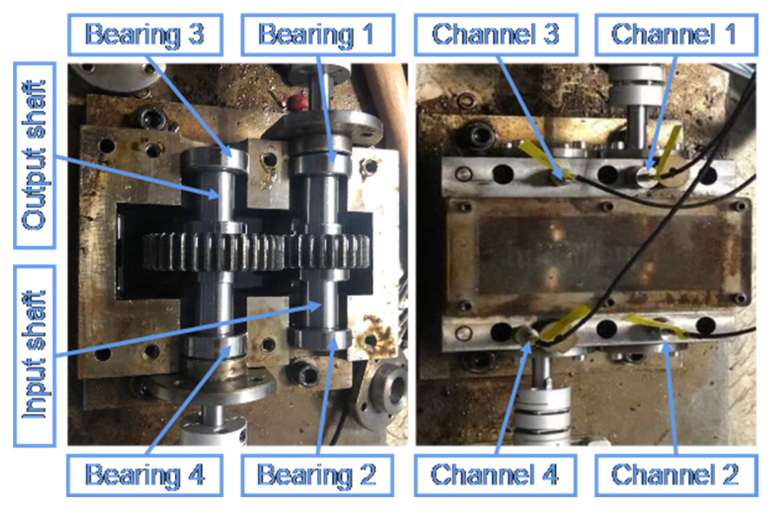
Experiments were conducted using the typical fault simulation test bench for bearings in a fixed-axis gear reducer at the State Key Laboratory of Mechanical System and Vibration at Shanghai Jiao Tong University. The experimental setup, as shown in Figure 17, mainly consists of a transmission platform, a control platform, and a data acquisition system. The gear reducer is equipped with four bearings. To obtain more realistic bearing vibration signals, four measurement points were set up at the input and output ends of the high-speed shaft and the input and output ends of the low-speed shaft of the gear reducer. Acceleration sensors (PCB352C04) were installed at each measurement point, with each sensor serving as a signal acquisition channel. Thus, four-channel fault signal data can be collected from these four measurement points. The installation positions of the bearings and sensors on the test bench are shown in Figure 17. Under healthy conditions, all bearings and other components in the gear reducer are considered to operate under normal conditions. Under fault conditions, an outer race fault bearing (type 7203) was installed on the low-speed shaft. The bearing was treated with localized pitting using electrical discharge machining, resulting in a weak fault. The sampling rate was 51,200 Hz, and the low-speed shaft was first accelerated and then decelerated, with a total of 37 s of data collected. This article extracts the acceleration time period data from 12 to 16 s as the analysis signal and extracts fault features from it. The experimental bearing parameters are shown in

Table 2. Test bearing parameters.

Type	Pitch Diameter (mm)	Rolling Element Diameter (mm)	Number of Rolling Elements	Contact Angle (°)
7203	28.5	7.14	10	15

.

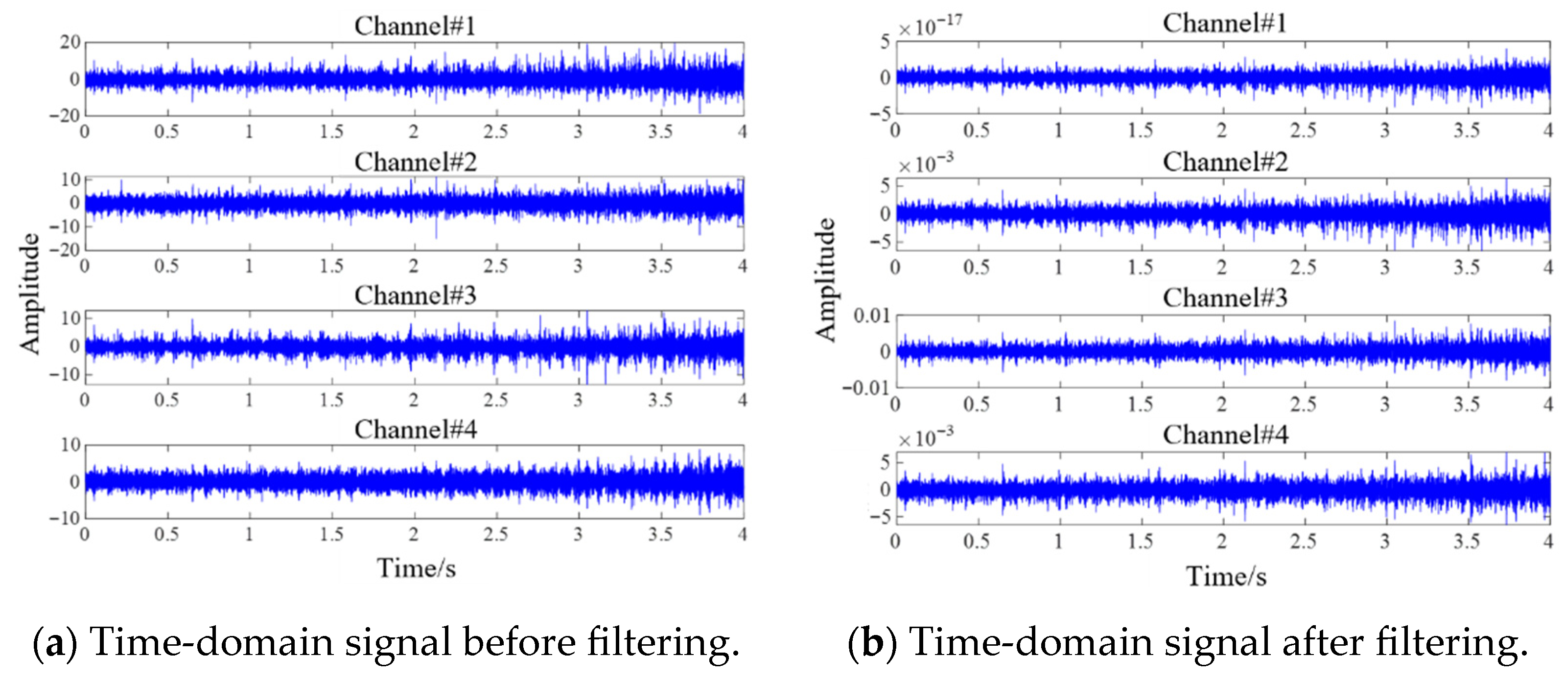
The four-channel data collected in the experiment are shown in Figure 18a, and it can be seen that the time-domain signals of the four channels are completely submerged by noise. To avoid mixing the meshing frequency of gears with the periodic pulse signal of faulty bearings, we need to filter the original signal using FIR filters. Due to the resonance frequency band being approximately 12,000 Hz, the setting parameters for the FIR filter are as follows: filter order is set to 256, window function is a Hamming window, centre frequency is 12,000 Hz, and bandwidth is 1000 Hz. 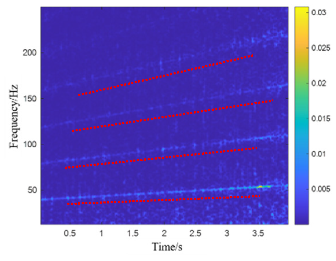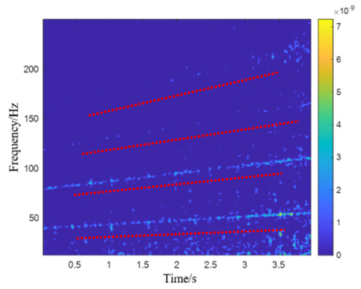The filtered four-channel data are shown in Figure 18b. A tensor construction method based on STFT is used to transform the four-channel fault signal into a time–frequency representation, as shown in Figure 19. The fault characteristic frequency of the bearing outer race can be barely distinguished from it, but the fault characteristics are still drowned out by background noise, especially the time–frequency representation matrix of channel#4, where the fault characteristics are almost indistinguishable.

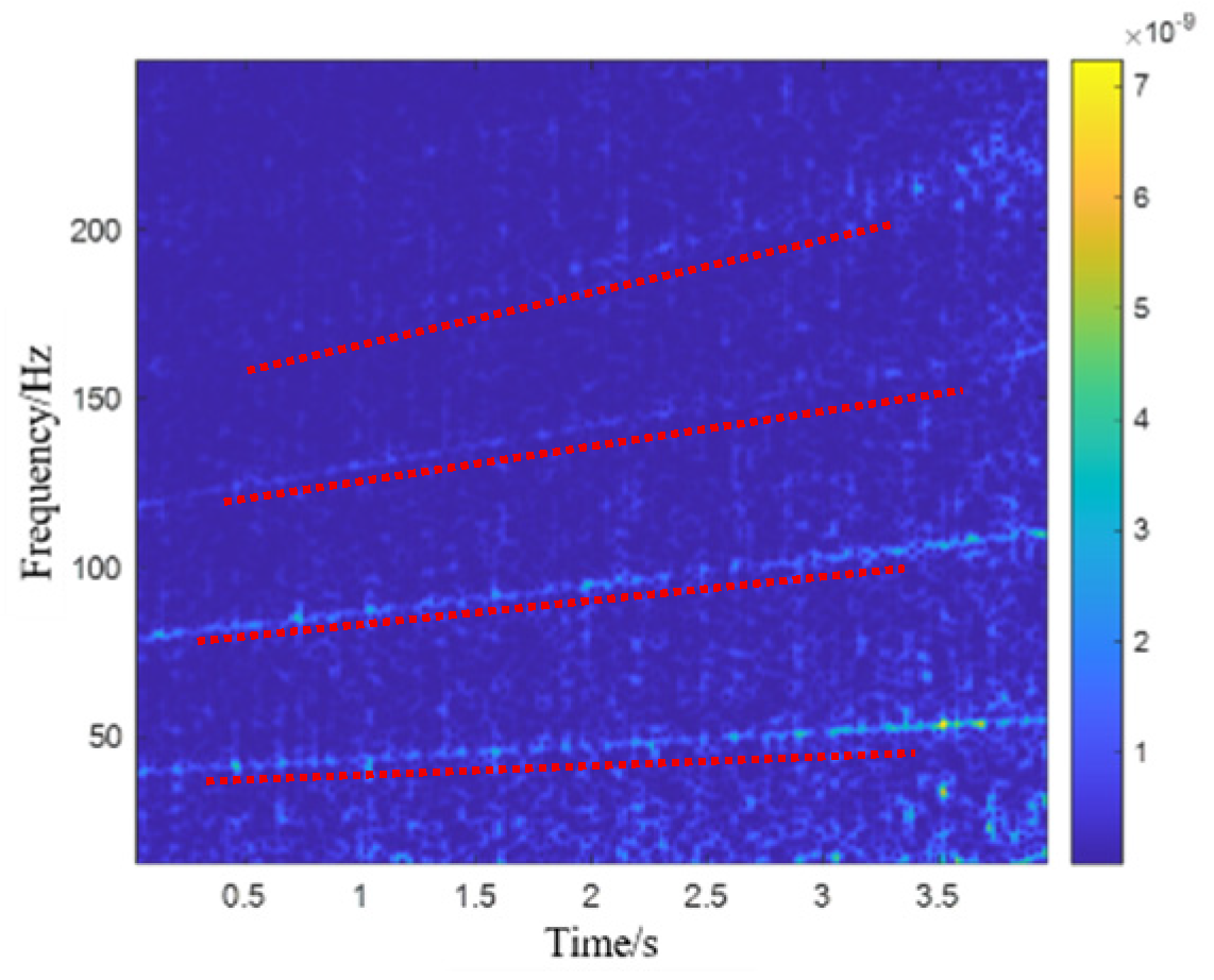
In order to verify the effectiveness of the proposed method for extracting fault features from complex background noise environments under variable-speed conditions, the bearing fault feature extraction method under variable-speed conditions was applied to the experimental signal with a maximum iteration of $k_{\max }$ = 500. Similarly, we first transformed the four-channel signal into a time–frequency representation using the STFT transform method, and arranged it along the number of channels to form a high-order time–frequency tensor. Next, the low-rank and sparsity co-induced tensor singular space decomposition method proposed in this study is used to extract the fault feature tensor, and use the global energy weighted fusion method to obtain the fusion matrix of the fault feature tensor, which helps us diagnose bearing fault features.

The fault feature extraction results extracted by this method and fusion matrix are shown in Figure 20 and Figure 21, respectively. It can be seen that the method proposed in this study effectively separates the fault characteristics. In the separated time–frequency representation, the outer race fault characteristics of the bearing can be clearly seen, and the frequency of the outer race fault characteristics has good continuity, effectively removing background noise. And, in the case where it is almost impossible to identify the fault characteristics for channel#4, this method utilizes the structural correlation between multiple channels and can still extract the outer race fault features well.

In order to verify the superiority of proposed method, TRPCA method, traditional tensor singular space decomposition method, and adaptive low-rank-induced tensor singular space decomposition method were also used to analyse the experimental data and compare them with the results of this study. The fault feature results extracted based on TRPCA method are shown in Figure 22 and Figure 23. It can be seen that although this method enhances some fault features, it cannot effectively remove background noise. The results of extracting fault features using traditional tensor singular space decomposition method are shown in Figure 24 and Figure 25. It can be seen that compared to the original data, the feature extraction effect of traditional methods is not very good, and the interference noise near the fault feature frequency and its harmonic components has not been completely removed. This indicates that the characteristics of fault features within the tensor are not fully precisely constrained, and the traditional method cannot achieve good feature extraction results. The results of extracting fault features using the decomposition method with only low-rank constraints are shown in Figure 26 and Figure 27. Compared with the traditional tensor singular space decomposition method, its effect has been significantly improved, indicating that the improvement of low-rank constraints is effective. However, the overall effect is still slightly worse than the method proposed in this paper. For the low-frequency part, the interference of noise cannot be completely removed, and the best feature extraction effect cannot be achieved. The model proposed in this study further improves the constraint conditions for inducing the sparsity of fault features, enabling the proposed method to enhance the structural correlation of sparsity between slices before and after fault features while removing noise. Therefore, the method proposed in this study has a good effect on fault feature extraction under the conditions of strong environmental noise interference and unclear fault features in this experiment.

The MSGI indicators corresponding to the above methods are shown in

Table 3. The MSGI of each method in test analysis.

Method	The Proposed Method	The TRPCA Method	The Traditional Tensor Singular Space Decomposition Method	The Adaptive Low-Rank-Induced Tensor Singular Space Decomposition Method
MSGI	0.8578	0.6725	0.7089	0.8063

. From the table, we can see that the MSGI of the method proposed in this paper is much higher than that of the other three compared methods, indicating that the sparsity of the extracted fault fusion time–frequency matrix is the best.

6. Conclusions

This study addresses the challenge of extracting bearing weak fault features under strong background noise interference under variable-speed conditions by proposing a novel weak fault feature extraction method based on tensor decomposition model. First, the time–frequency tensor is constructed based on the short-time Fourier transform. Then, two types of fault property in tensor are explored and an improved tensor decomposition model is proposed to realize the accurate extraction of weak fault features under variable-speed conditions. In addition, the decomposed feature tensor is conducted by multichannel global energy-weighted fusion strategy, which significantly improves the robustness in extracting multichannel weak fault features.

Simulation of multichannel variable-speed signals and laboratory experiments demonstrate that the proposed method outperforms other methods. First, the proposed method is compared with the TRPCA method, validating the superiority of the low-rank and sparsity co-induced decomposition method. Second, a comparison with the traditional tensor singular space decomposition method verifies the superiority of the adaptive threshold function in constraining the low-rank properties of tensor singular space. Third, a comparison with the adaptive low-rank-induced tensor singular space decomposition method confirms the superiority of the 112-norm in constraining sparsity. In summary, this study provides a new theoretical tool for fault diagnosis of rotating machinery under variable operating conditions and offers a reference for multichannel/multisensory signal processing research in the era of Industry 4.0. The core ideas can be transferred to health monitoring fields of high-end equipment such as wind power and high-speed rail, demonstrating significant engineering application prospects.