Three-Dimensional Mathematical Modeling and Simulation of the Impurity Diffusion Process Under the Given Statistics of Systems of Internal Point Mass Sources

Abstract

A three-dimensional mathematical model and simulation of the impurity diffusion process are developed under the given statistical characteristics of the system of internal stochastically disposed point sources of mass. These sources, possessing varying intensities, are located within the sub-strip according to a uniform distribution. The random source statistics are known, and the problem solution is expressed as the sum of the solution to the homogeneous problem and the convolution of Green’s function with the random point source system. The impurity concentration is averaged. Diffusive fluxes and the total amount of substance passing through any cross-sectional area over a specified time period are modeled using Fick’s laws. General and calculating formulas for averaged diffusive fluxes, including those applicable to steady-state regimes, are derived. A calculating formula for the total substance that has passed through the strip within a given time interval is obtained. A comprehensive software suite is developed to simulate the behavior of the averaged characteristics of the diffusion process influenced by the point source system. The second statistical moments of the impurity concentration are obtained and studied.

1. Introduction

In mathematical modeling of physical processes in multicomponent or multiphase media, scientists encounter problems due to insufficient knowledge on the internal structure of the investigated objects [1]. In such situations, to adequately describe the processes, it is important to account for stochasticity caused by uncertainty in the location of internal mass sources or due to the influence of random external factors. This is also characteristic of diffusion problems [2]. Even on its own, diffusion remains an active area of mathematical research, with advancements being made both in the development of new mathematical models [3] and in the creation of more stable and efficient numerical solution techniques [4].

Of significant interest are problems that take into account the action of internal point mass sources. Such problems often arise from chemical reactions, crystallization, melting, or other physical phenomena where mass sources play a key role. Often, the specific location of these sources is unknown, which adds random parameters to the problem. These challenges appear in the areas of building industry, machine and aircraft engineering, agriculture, ecology, and the longevity and reliability of devices’ operation as well as units and elements of complex constructions. For example, such problems are solved when investigating the motion and stability of systems of point masses in the context of gravitational interactions or in the analysis of the distribution of radioactive radiation.

In such cases, the processes are described using the probabilistic modeling approach, which is widely applied for analyzing complex physical and technical systems, encompassing both deterministic and probabilistic problems. The main advantage of this approach lies in its ability to model uncertainties and consider probability distributions, which is critical for problems where uncertainty exists, such as in the location of mass sources during diffusion [5,6]. However, choosing an adequate model remains a challenge that requires a deep understanding of both the physical aspects of the studied process and the applied mathematical approaches [7].

For a long time, methods for homogenizing heterogeneous media—including those with randomly heterogeneous structures [8]—have been rapidly evolving. However, such approaches do not allow one to determine the variance or the correlation function of the concentration field of the diffusing substance, nor do they account for the complete statistics of random sources acting within the investigated object [9].

This work aims to design a three-dimensional mathematical model that describes the diffusion of impurities affected by a system of internal stochastic point sources of impurity in a strip. The statistics of these point sources are assumed to be known in advance. Building on this foundation, we construct the solution to the initial-boundary value problem for diffusion and numerically examine the solution, namely the averaged concentration field of the particles diffusing. From there, we proceed to analyze critical characteristics of the mass transfer process, including impurity flux, the total substance passing through a defined strip, and the second moments of the concentration field.

2. Materials and Methods

The mass transfer equation for the impurity concentration is derived using the mass conservation laws from the thermodynamics of non-equilibrium processes. Impurity concentration formulas, flux in a homogeneous medium (without mass sources), and the Green function are obtained through the application of integral transform methods. Specifically, the Fourier transform is applied relative to the spatial coordinates, and the Laplace transform is applied to time. The resulting solution is presented in analytical form. To perform the averaging procedure over the random positions of point mass sources, tools from probability theory and statistics as well as calculus are utilized.

The developed software suite for the numerical representation and analysis consists of the following modules:

• Problem parameter interpreter module;
• Homogeneous concentration and Green’s function calculation module;
• Flux function evaluation module;
• Stochastic characteristics computation module;
• Two- and three-dimensional visualization module.

These modules were implemented using the C# programming language in Visual Studio 2022 Community Edition. The visualization was performed using the Plottly.Net@5.1.0 and ScottPlot@4.1.68 libraries. The software was run on the following hardware configuration: Windows 11 Pro OS 64-bit, Intel(R) Core(TM) i7-1065G7 CPU, 16.0 GB RAM.

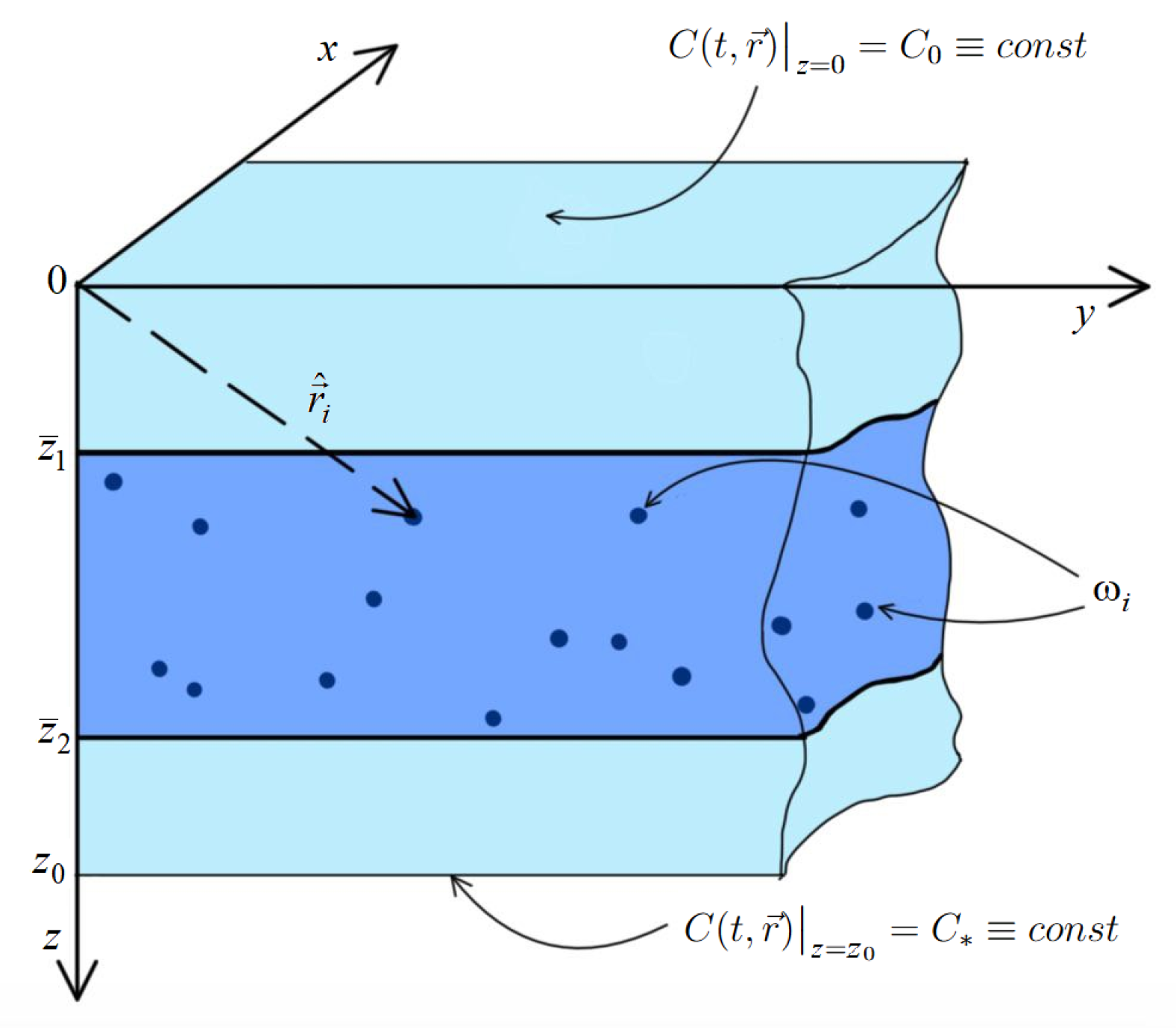
3. Mathematical 3D Model of Impurity Diffusion Influenced by Point Source System

3.1. Construction of the Mathematical Model

A three-dimensional layer with a thickness of $z_0$ forms the domain where an impurity substance diffuses. Consider a set of random points $\overrightarrow{r}={\widehat{\overrightarrow{r}}}_i$, within the body region, where $\overrightarrow{r}=(x,y,z)$ is the radius vector of the current point, ${\widehat{x}}_i,{\widehat{y}}_i\in (-\infty ,\infty )$, and ${\widehat{z}}_i\in [{\overline{z}}_1,{\overline{z}}_2]\subset [0,z_0]$. Located in those points is a set of acting mass sources ${\omega }_i\delta (\overrightarrow{r}-{\widehat{\overrightarrow{r}}}_i)$, ${\omega }_i$ is the power of the i-th source, $i=1,2,\dots ,n$, with n representing the number of random point sources, and $\delta (\overrightarrow{r}-{\widehat{\overrightarrow{r}}}_i)=\delta (x-{\widehat{x}}_i)\delta (y-{\widehat{y}}_i)\delta (z-{\widehat{z}}_i)$ is the delta function. The collection of sources is regarded as a system (Figure 1).

Let $i,j,k=1,\dots ,n$. The sources’ statistics are then defined as $\langle \delta (\overrightarrow{r}-{\widehat{\overrightarrow{r}}}_i)\rangle$, $\langle \delta (\overrightarrow{r}-{\widehat{\overrightarrow{r}}}_i)\delta (\overrightarrow{r}-{\widehat{\overrightarrow{r}}}_j)\rangle$, $\langle \delta (\overrightarrow{r}-{\widehat{\overrightarrow{r}}}_i)\delta (\overrightarrow{r}-{\widehat{\overrightarrow{r}}}_j)\delta (\overrightarrow{r}-{\widehat{\overrightarrow{r}}}_k)\rangle$, …

When formulating the initial relationships of the mathematical model for mass transfer of impurity particles, we assume that any arbitrary region of the body consists of two parts: a skeleton and an impurity component. The mass transfer process occurs solely through diffusion. It is assumed that during the mass transfer, the skeleton does not deform. Additionally, we assume that the medium is isotropic. Based on these assumptions, we construct the mass balance equations for each component [10].

$$\rho {\displaystyle \frac{d{C}_k}{dt}}=-\overrightarrow{\nabla }·{\overrightarrow{J}}_k+{\sigma }_{mk},k=0,1;$$

(1)

where $\rho$ is the body’s total density, $C_k$ is the mass concentration of component k, ${\overrightarrow{J}}_k$ is the diffusive flux of the component k, ${\sigma }_{mk}$ is the mass production rate of the component k of the body, and $d/dt=\partial /\partial t+{\nu }_r·\overrightarrow{\nabla }$ represents the total time derivative. Here, the particles of the body’s skeleton are assigned the index $k=0$, and the impurity particles are assigned the index $k=1$.

The diffusion flux ${\overrightarrow{J}}_k$ is determined by the gradients of chemical potentials, which are linearly dependent on concentrations [11], i.e.,

$${\overrightarrow{J}}_k=-L_k\overrightarrow{\nabla }{C}_k,k=0,1;$$

where $L_k$ are the transport kinetic coefficients. The concentrations $C_k$ and fluxes ${\overrightarrow{J}}_k$ satisfy the normalization conditions ${\sum }_k{C}_k=1$ and ${\sum }_k{\overrightarrow{J}}_k=0$. The density and kinetic coefficients are assumed to be constant.

For the component $k=0$, the mass production rate ${\sigma }_{m0}=0$. At the same time, the mass production rate of the impurity substance ${\sigma }_{m1}={\sigma }_{m1}(r,{\widehat{\overrightarrow{r}}}_i)$ is a random function of the spatial coordinates corresponding to the locations of internal point sources.

3.2. Formulation of the Initial–Boundary Value Problem for Diffusion

Let the mass production rate be represented as a sum of the sources:

$${\sigma }_{m1}=\sum _{i=1}^n{\omega }_i\delta (\overrightarrow{r}-{\widehat{\overrightarrow{r}}}_i),$$

then the equation for the diffusion of the impurity substance influenced by the point source system, in three dimensions with respect to spatial variables, is derived from (1) as follows:

$$\rho {\displaystyle \frac{\partial C(t,\overrightarrow{r})}{\partial t}}=d{\Delta }_{\overrightarrow{r}}C(t,\overrightarrow{r})+\sum _{i=1}^n{\omega }_i\delta (\overrightarrow{r}-{\widehat{\overrightarrow{r}}}_i),$$

(2)

where d is the kinetic transfer coefficient and t is time. Moreover, the index denoting the impurity $k=1$ will be omitted from now on, i.e., $C_1(t,\overrightarrow{r})=C(t,\overrightarrow{r})$. Here, we neglected the convective transfer component.

Let the boundary and initial conditions of the first type be imposed. Namely, we assume zero initial conditions, and we enforce a constant concentration of the particles on both boundaries of the strip:

$$\begin{array}{cc}\hfill & C(t,\overrightarrow{r}){|}_{t=0}=0,\hfill \end{array}$$

(3)

$$\begin{array}{cc}\hfill & C(t,\overrightarrow{r}){|}_{z=0}=C_0\equiv const,C(t,\overrightarrow{r}){|}_{z=z_0}=C_{*}\equiv const,\hfill \end{array}$$

(4)

$$\begin{array}{cc}\hfill & C(t,\overrightarrow{r}){|}_{x\to \pm \infty ,y\to \pm \infty }\le M<\infty .\hfill \end{array}$$

(5)

The action of the system of random point mass sources in the body induces randomness in the impurity concentration, or more broadly, the stochasticity of the sought functions.

4. Construction of the Solution to the 3D Problem of Impurity Diffusion Influenced by the Stochastic Point Source System

4.1. Integral Transforms

We will construct the solution to the initial–boundary value problem (2)–(5) as a combination of the solution to the homogeneous problem and the convolution of Green’s function with the system of stochastic point sources of mass. So, we obtain

$$C(t,\overrightarrow{r})=C^h(t,\overrightarrow{r})+\sum _{i=1}^n{\omega }_i{\int }_0^t{\int \int \int }_{\left(V\right)}G(t,t^{\prime },\overrightarrow{r},{\overrightarrow{r}}^{\prime })\delta ({\overrightarrow{r}}^{\prime }-{\widehat{\overrightarrow{r}}}_i)d^3{\overrightarrow{r}}^{\prime }d{t}^{\prime },$$

(6)

where $C^h(t,\overrightarrow{r})=C^h(t,z)$ is the homogeneous problem’s solution. Here, we take into account the symmetry relative to the variables y and z and thus obtain

$$\rho {\displaystyle \frac{\partial C^h(t,z)}{\partial t}}=d{\displaystyle \frac{{\partial }^2{C}^h(t,z)}{\partial z^2}},$$

(7)

$$\begin{array}{cc}\hfill & C^h(t,z){|}_{t=0}=0,\hfill \end{array}$$

(8)

$$\begin{array}{cc}\hfill & C^h(t,z){|}_{z=0}=C_0\equiv const,C^h(t,z){|}_{z=z_0}=C_{*}\equiv const,\hfill \end{array}$$

(9)

namely [10,12]

$$\begin{array}{cc}\hfill C^h(t,z)& =C_0\left(1-{\displaystyle \frac{z}{z_0}}\right)+C_{*}{\displaystyle \frac{z}{z_0}}\hfill \\ \hfill & -{\displaystyle \frac{2}{z_0\rho }}\sum _{k=1}^{\infty }{\displaystyle \frac{1}{z_k}}\left(C_0+{(-1)}^{k+1}{C}_{*}\right)e^{-d{z}_k^{2}t/\rho }sin\left(z_{k}z\right),\hfill \end{array}$$

(10)

where $z_k=\pi k/z_0$, $k=1,2,\dots$ Another component of (6) is $G(t,t^{\prime },\overrightarrow{r},{\overrightarrow{r}}^{\prime })$, the Green function of problems (2)–(5), which is the solution to the next zero boundary and zero initial condition problem

$$\rho {\displaystyle \frac{\partial G(t,t^{\prime },\overrightarrow{r},{\overrightarrow{r}}^{\prime })}{\partial t}}-d{\Delta }_{\overrightarrow{r}}G(t,t^{\prime },\overrightarrow{r},{\overrightarrow{r}}^{\prime })=\delta (t-t^{\prime })\delta (\overrightarrow{r}-{\overrightarrow{r}}^{\prime }),$$

(11)

$$\begin{array}{c}G(t,t^{\prime },\overrightarrow{r},{\overrightarrow{r}}^{\prime }){|}_{t=0}=0,\end{array}$$

(12)

$$\begin{array}{c}G(t,t^{\prime },\overrightarrow{r},{\overrightarrow{r}}^{\prime }){|}_{z=0}=0,G(t,t^{\prime },\overrightarrow{r},{\overrightarrow{r}}^{\prime }){|}_{z=z_0}=0,\end{array}$$

(13)

$$\begin{array}{c}G(t,t^{\prime },\overrightarrow{r},{\overrightarrow{r}}^{\prime }){|}_{x\to \pm \infty ,y\to \pm \infty }=0.\end{array}$$

(14)

After applying Laplace [13] and finite sine–Fourier integral transforms [14,15], specifically $G(t,t^{\prime },x,y,z,{\overrightarrow{r}}^{\prime })\to \tilde{g}(s,t^{\prime },p_1,p_2,z_k,{\overrightarrow{r}}^{\prime })$, we obtain

$$\tilde{g}(\rho s+d{p}_1^2+d{p}_2^2+d{z}_k^2)=e^{i{p}_1{x}^{\prime }+i{p}_2{y}^{\prime }}{e}^{-s{t}^{\prime }}sin\left(z_k{z}^{\prime }\right).$$

The solution to this equation is

$$\tilde{g}={\displaystyle \frac{e^{i{p}_1{x}^{\prime }+i{p}_2{y}^{\prime }}sin\left(z_k{z}^{\prime }\right)e^{-s{t}^{\prime }}}{\rho s+d{p}_1^2+d{p}_2^2+d{z}_k^2}}.$$

We apply the inverse Laplace and Fourier integral transforms together with the Time Delay theorem. So, we have

$$\begin{array}{cc}\hfill G(t,t^{\prime },\overrightarrow{r},{\overrightarrow{r}}^{\prime })& ={\displaystyle \frac{\theta (t-t^{\prime })}{z_{0}d(t-t^{\prime })}}exp\left\{-{\displaystyle \frac{\rho }{4d}}{\displaystyle \frac{{(x-x^{\prime })}^2+{(y-y^{\prime })}^2}{t-t^{\prime }}}\right\}\hfill \\ \hfill & \times \sum _{k=1}^{\infty }{e}^{-d{z}_k^2(t-t^{\prime })/\rho }sin\left(z_k{z}^{\prime }\right)sin\left(z_{k}z\right).\hfill \end{array}$$

(15)

Here, $\theta (t-t^{\prime })$ is the Heaviside function.

Note that integration in (6) is performed in the region $\left(V\right)=[0;z_0]\times [-\infty ;\infty ]\times [-\infty ;\infty ]$.

4.2. Averaging the Concentration over the Random Source Locations

The next step is the averaging of the concentration $C(t,\overrightarrow{r})$ with respect to the stochastic positions ${\widehat{\overrightarrow{r}}}_i$ of the point sources. Given that $C^h(t,\overrightarrow{r})$ is deterministic, it follows that $\langle C^h(t,\overrightarrow{r})\rangle =C^h(t,\overrightarrow{r})$. Subsequently,

$$\langle C(t,\overrightarrow{r})\rangle =C^h(t,\overrightarrow{r})+〈\sum _{i=1}^n{\omega }_i{\int }_0^t{\int \int \int }_{\left(V\right)}G(t,t^{\prime },\overrightarrow{r},{\overrightarrow{r}}^{\prime })\delta ({\overrightarrow{r}}^{\prime }-{\widehat{\overrightarrow{r}}}_i)d^3{\overrightarrow{r}}^{\prime }d{t}^{\prime }〉,$$

(16)

where ${\widehat{\overrightarrow{r}}}_i=({\widehat{x}}_i,{\widehat{y}}_i,{\widehat{z}}_i)$ and the angle brackets denote the averaging procedure.

Let us consider the set of random point mass sources ${\omega }_i\delta (\overrightarrow{r}-{\widehat{\overrightarrow{r}}}_i)$ that act within the body in greater detail. As per our previous assumption, the sources form the system. Let $p\left({\widehat{\overrightarrow{r}}}_i\right)$ be the likelihood of finding the source in a specific location within the body region, namely the probability density function. It is assumed that each source contributes to the system with equal probability. Then, the function $p\left({\sum }_{i=1}^n{\widehat{\overrightarrow{r}}}_i\right)$ can be expressed as a sum of the probability densities $p\left({\widehat{\overrightarrow{r}}}_i\right)$ with unit weights ${\alpha }_i$:

$$p\left(\sum _{i=1}^n{\widehat{\overrightarrow{r}}}_i\right)=\sum _{i=1}^n{\alpha }_{i}p\left({\widehat{\overrightarrow{r}}}_i\right),{\alpha }_i\equiv 1.$$

(17)

Let the internal region of the body, where the system of sources operates, be known as $[{\overline{z}}_1;{\overline{z}}_2]\times [-\infty ;\infty ]\times [-\infty ;\infty ]\subseteq [0;z_0]\times [-\infty ;\infty ]\times [-\infty ;\infty ]$ (Figure 1). Consider the case of the continuous uniform distribution of the random vector ${\widehat{\overrightarrow{r}}}_i$ of the point source disposition. Allowing for Expression (17), the averaged field of concentration $\langle C(t,\overrightarrow{r})\rangle$ is represented as

$$\begin{array}{cc}\hfill \langle C(t,\overrightarrow{r})\rangle & =C^h(t,z)+\sum _{i=1}^n{\omega }_i{\int }_{{\overline{z}}_1}^{{\overline{z}}_2}d{\widehat{z}}_i{\int \int }_{-\infty }^{\infty }p\left({\widehat{\overrightarrow{r}}}_i\right)d{\widehat{x}}_{i}d{\widehat{y}}_i\hfill \\ \hfill & \times {\int }_0^{t}G(t,t^{\prime },\overrightarrow{r},{\widehat{\overrightarrow{r}}}_i)d{t}^{\prime }.\hfill \end{array}$$

(18)

This leads to

$$\begin{array}{cc}\hfill \langle C(t,\overrightarrow{r})\rangle & =C^h(t,z)+\sum _{i=1}^n{\displaystyle \frac{{\omega }_i}{V{z}_{0}d}}\sum _{k=1}^{\infty }sin\left(z_{k}z\right){\int }_{{\overline{z}}_1}^{{\overline{z}}_2}sin\left(z_k{\widehat{z}}_i\right)d{\widehat{z}}_i\hfill \\ \hfill & \times {\int }_0^t{\displaystyle \frac{1}{t-t^{\prime }}}{e}^{-d{z}_k^2(t-t^{\prime })/\rho }{\int }_{-\infty }^{\infty }exp\left\{-{\displaystyle \frac{\rho }{4d}}{\displaystyle \frac{{(x-{\widehat{x}}_i)}^2}{t-t^{\prime }}}\right\}d{\widehat{x}}_i\hfill \\ \hfill & \times {\int }_{-\infty }^{\infty }exp\left\{-{\displaystyle \frac{\rho }{4d}}{\displaystyle \frac{{(y-{\widehat{y}}_i)}^2}{t-t^{\prime }}}\right\}d{\widehat{y}}_{i}d{t}^{\prime },\hfill \end{array}$$

where V is the volume of the body.

When averaging with a uniform distribution, one faces an inconsistency between the physical object and the mathematical model, which describes an infinite body with a finite number of sources acting within it. Thus, we consider

$$\begin{array}{cc}\hfill {\displaystyle \frac{1}{V}}& ={\displaystyle \frac{n\mathrm{mes}0({\overline{z}}_2-{\overline{z}}_1)}{Vn\mathrm{mes}0({\overline{z}}_2-{\overline{z}}_1)}}={\displaystyle \frac{V_1}{Vn\mathrm{mes}0({\overline{z}}_2-{\overline{z}}_1)}}\hfill \\ \hfill & ={\displaystyle \frac{v_1}{n\mathrm{mes}0({\overline{z}}_2-{\overline{z}}_1)}}={\displaystyle \frac{1}{2\pi n({\overline{z}}_2-{\overline{z}}_1)}},\hfill \end{array}$$

(19)

where $V_1=n\mathrm{mes}0({\overline{z}}_2-{\overline{z}}_1)$ is the volume occupied by the system of point sources, mes 0 is a measure zero [16], and $v_1=V_1/V$ is the volume fraction of the point source system.

Substituting Green’s function (15) into (18), after integration, we obtain

$$\begin{array}{cc}\hfill \langle C(t,\overrightarrow{r})\rangle & =C^h(t,z)+{\displaystyle \frac{2\Omega }{d{z}_{0}n({\overline{z}}_2-{\overline{z}}_1)}}\hfill \\ \hfill & \times \sum _{k=1}^{\infty }{S}_{12}\left(z_k\right)\left(1-e^{-d{z}_k^{2}t/\rho }\right)sin\left(z_{k}z\right),\hfill \end{array}$$

(20)

where

$$S_{12}\left(z_k\right)={\displaystyle \frac{cos\left(z_k{\overline{z}}_1\right)-cos\left(z_k{\overline{z}}_2\right)}{z_k^3}},\Omega =\sum _{i=1}^n{\omega }_i.$$

(21)

It is noteworthy that the expressions for the averaged concentration in the three-dimensional and one-dimensional cases coincide [17], which can be attributed to the symmetry arising along the x and y axes.

5. Results

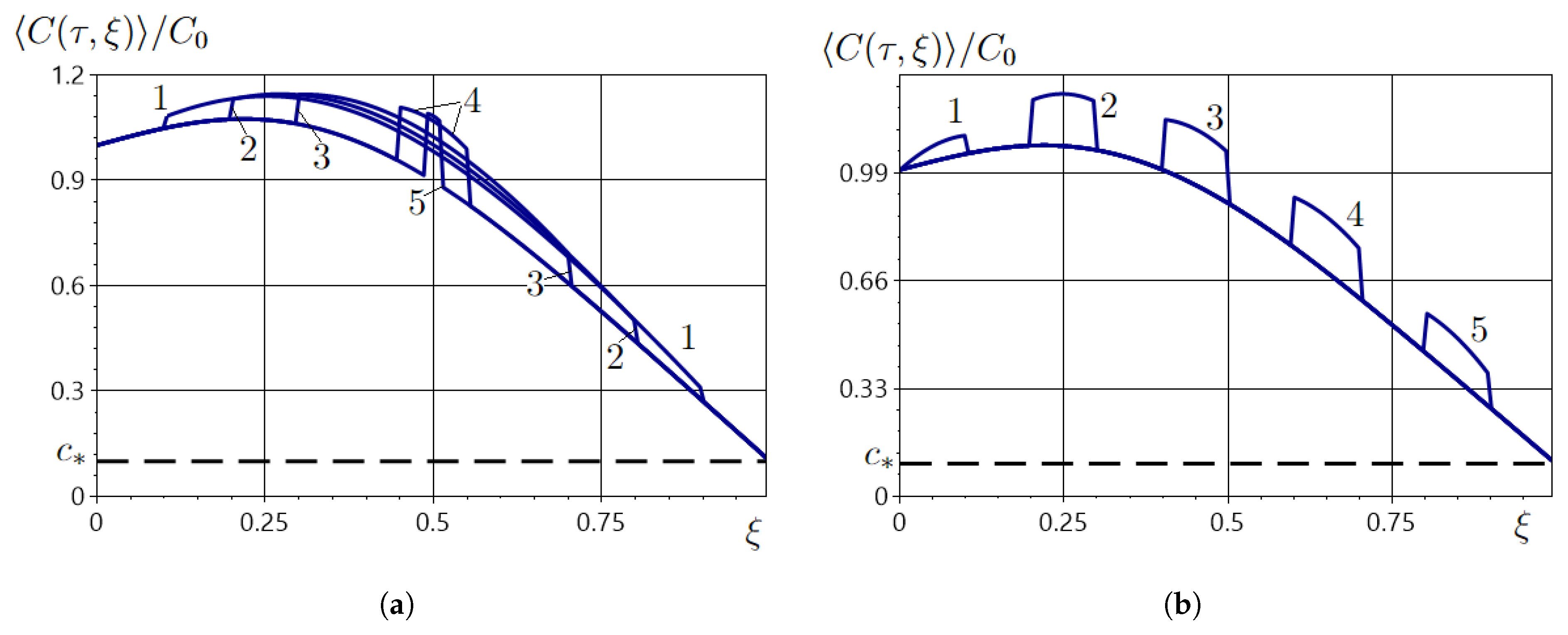
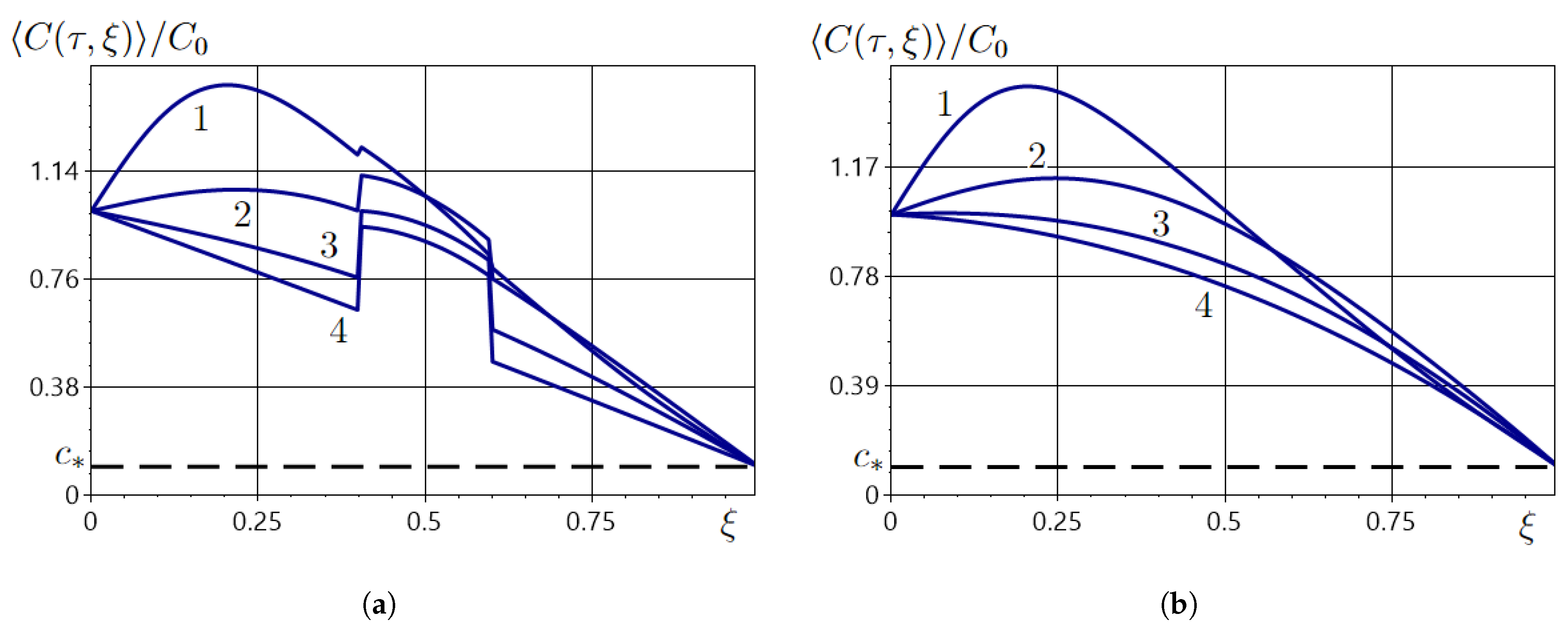
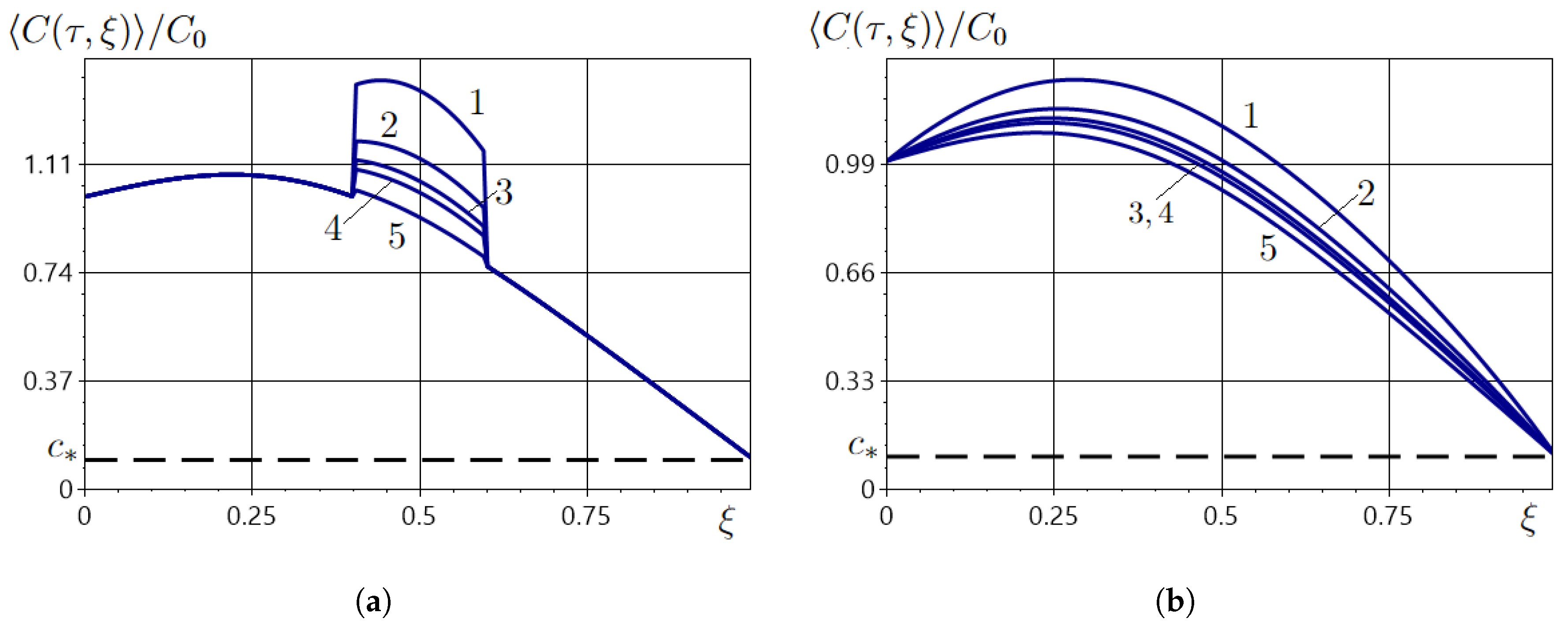
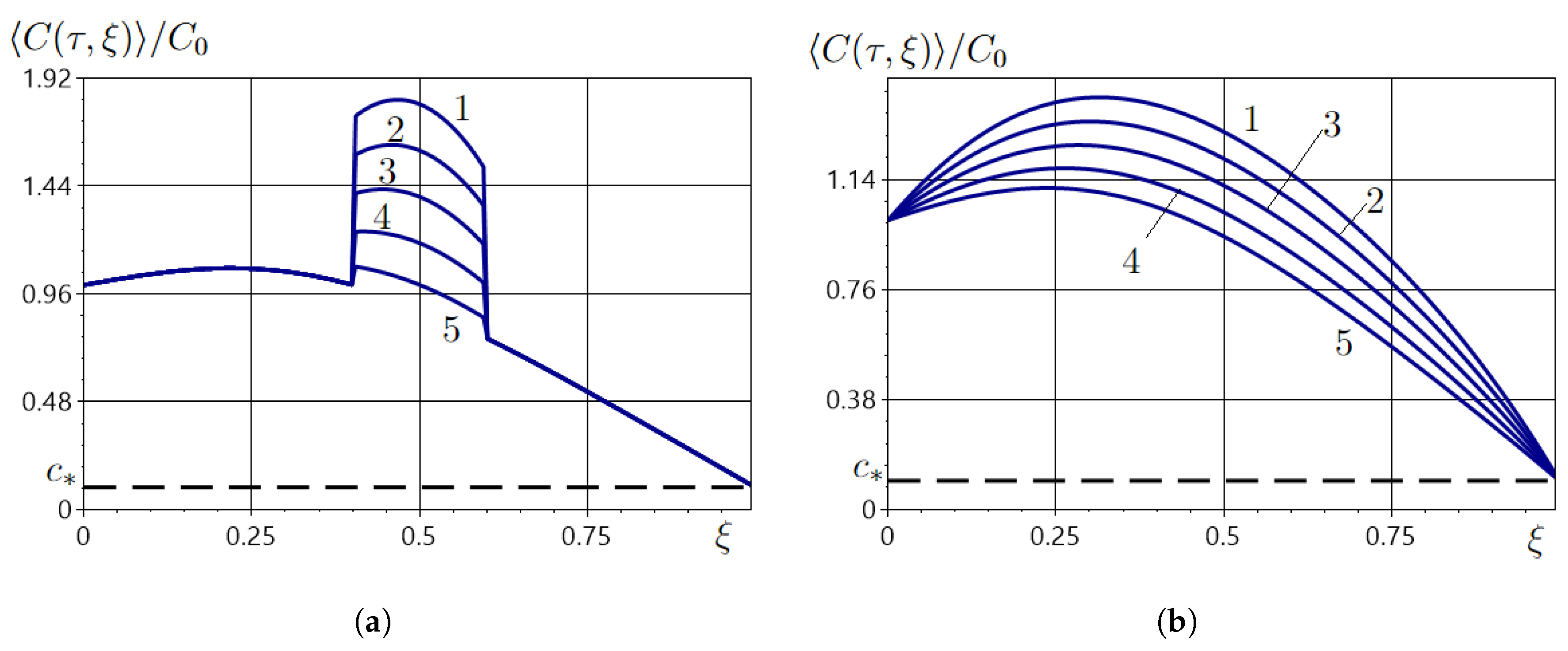
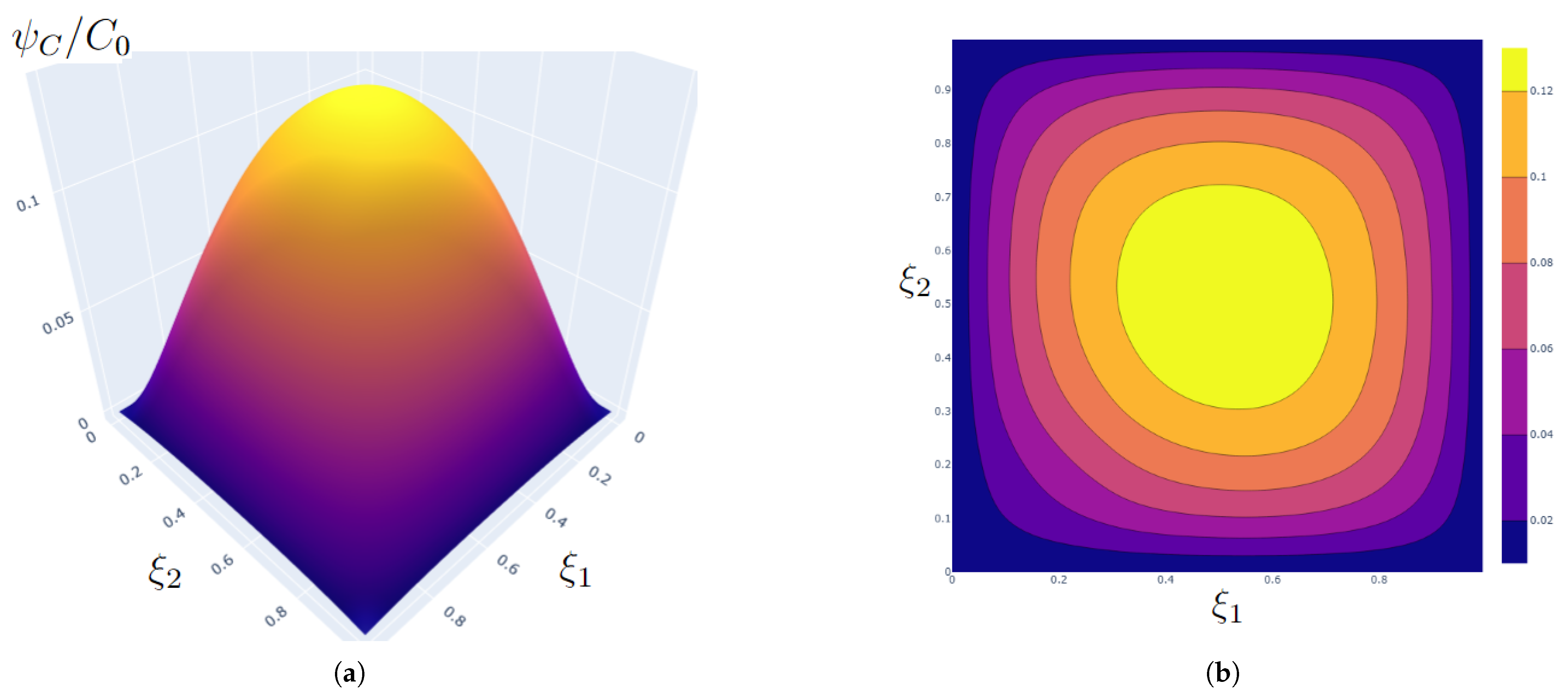
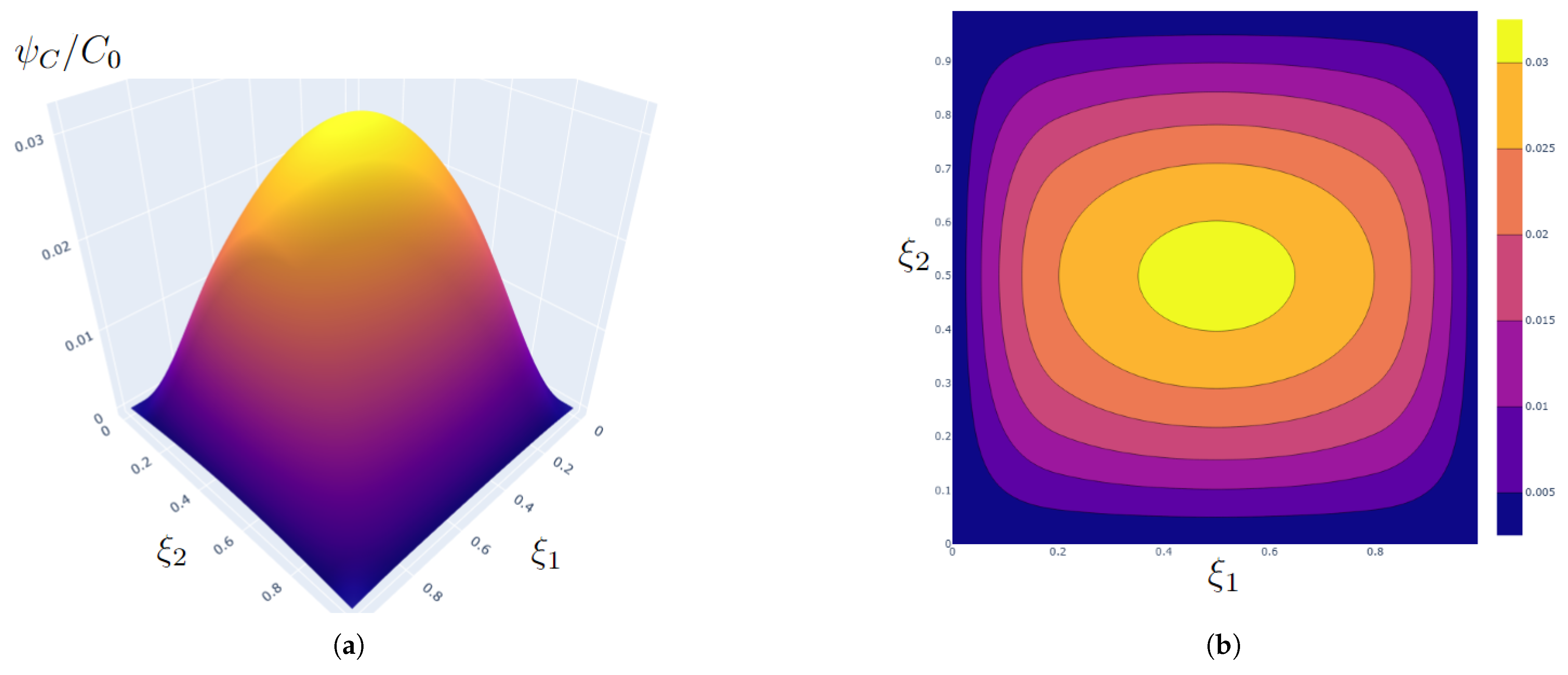
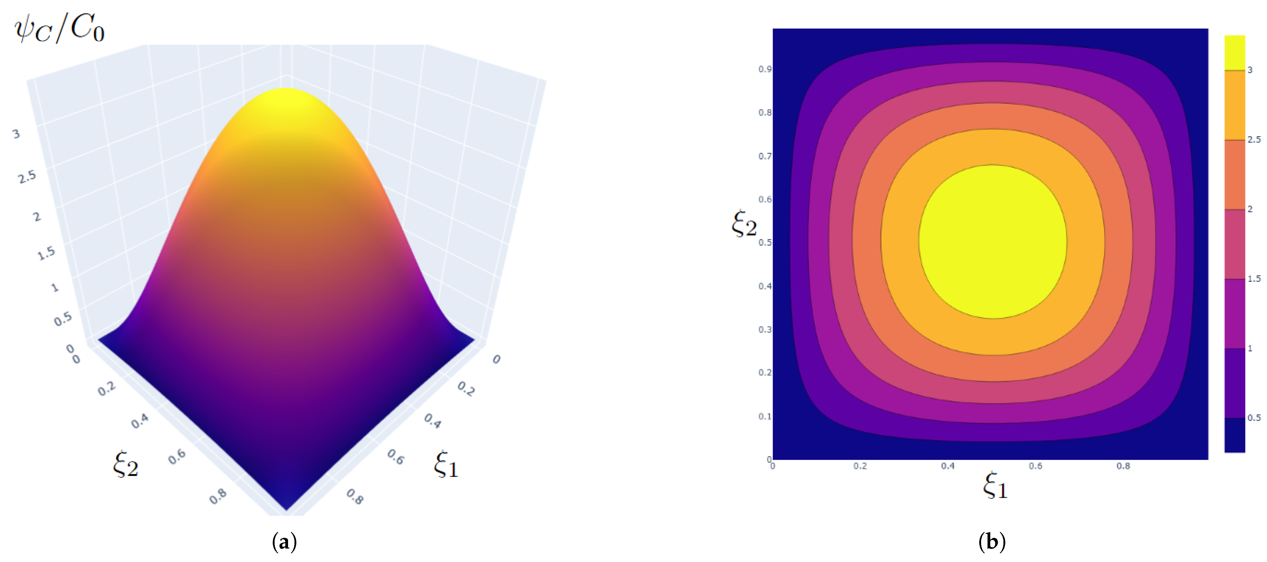
5.1. Numerical Analysis of the Averaged Field of the Impurity Concentration

Figure 2, Figure 3, Figure 4, Figure 5, Figure 6 and Figure 7 display the plots of the averaged function of impurity concentration $\langle C(\tau ,\xi )\rangle /C_0$, within a strip for a uniform distribution of random point sources constituting the system. Formula (20) was used for the calculations.

Here and throughout dimensionless variables [18], we utilize

$$\xi =z/z_0,\tau =d/\left(\rho z_0^2\right)t.$$

(22)

Consequently, the strip’s dimensionless thickness ${\xi }_0=1$, whereas internal interval edges ${\overline{\xi }}_1={\overline{z}}_1/z_0$ and ${\overline{\xi }}_2={\overline{z}}_2/z_0$.

The default values of the problem coefficients are taken as $d=1$, $\rho =1$, $n=3$, ${\omega }_1={\omega }_2={\omega }_3=1.5$, ${\overline{\xi }}_1=0.4$, ${\overline{\xi }}_2=0.6$, $C_0=1$, $C_{*}=0.1$, $\tau =0.05$. The system consisting of three point sources of equal power is investigated. The series in the formulas for the averaged concentration are summed with an accuracy of ${10}^{-12}$. Dashed horizontal lines in Figure 2, Figure 3, Figure 4, Figure 5, Figure 6 and Figure 7 mark the fixed concentration value $C_{*}$ at the boundary $\xi ={\xi }_0$.

Figure 2a shows the behavior of the averaged field $\langle C(\tau ,\xi )\rangle /C_0$ for various lengths of the section $[{\overline{\xi }}_1,{\overline{\xi }}_2]=[0.1,0.9];[0.2,0.8];[0.3,0.7];[0.45,0.55];[0.49,0.51]$ (corresponding to lines 1 through 5 on the graph).

Figure 2b demonstrates the graphs of the averaged field of concentration depending on the location of the interval of the source system $[{\overline{\xi }}_1,{\overline{\xi }}_2]$ within the body region: $[{\overline{\xi }}_1,{\overline{\xi }}_2]=[0,0.1];[0.2,0.3];[0.4,0.5];[0.6,0.7];[0.8,0.9]$ (corresponding to lines 1 through 5 on the graph).

Figure 3 presents the distributions of the averaged impurity concentration field at various dimensionless times $\tau =0.01,0.05,0.15,0.4$ (corresponding to curves 1–4). From this point onward, Figure 3a is plotted for the interval of the point source system’s action $[{\overline{\xi }}_1,{\overline{\xi }}_2]=[0.4,0.6]$, and Figure 3b is plotted for $[{\overline{\xi }}_1,{\overline{\xi }}_2]=[0,1]$.

Figure 4 presents the distributions of the averaged concentration $\langle C(\tau ,\xi )\rangle /C_0$ normalized by its value at the boundary $\xi =0$ for different values of the concentration maintained at the strip’s boundary $\xi ={\xi }_0$: $C_{*}=0,0.1,0.5,0.75,1.2$ (curves 1–5). Figure 5 shows the distributions of the averaged concentration $\langle C(\tau ,\xi )\rangle /C_{*}$, normalized by its value at the boundary $\xi ={\xi }_0$, depending on the value of $C(\tau ,\xi )$ on the upper surface $\xi =0$: $C_0=0,0.1,0.5,0.75,1.2$ (curves 1–5).

Figure 4 depicts the profiles of the averaged field of concentration $\langle C(\tau ,\xi )\rangle /C_0$ normalized by its value at the boundary $\xi =0$ for various concentrations imposed at the boundary $\xi ={\xi }_0$: $C_{*}=0,0.1,0.5,0.75,1.2$ (curves 1–5). Figure 5 shows the distributions of the averaged concentration $\langle C(\tau ,\xi )\rangle /C_{*}$, divided by its bottom boundary value at $\xi ={\xi }_0$, with various values of $C(\tau ,\xi )$ at the top boundary $\xi =0$, namely $C_0=0,0.1,0.5,0.75,1.2$ (curves 1–5).

Figure 6 shows the plots of the field $\langle C(\tau ,\xi )\rangle /C_0$ for the system of varying number of point sources with the same total power $\Omega =4.5$: $\omega =4.5$ (1 source), $2.25$ (2 sources), $1.5$ (3 sources), $1.125$ (4 sources) and $0.3$ (15 sources) which correspond to curves 1–5. Figure 7 demonstrates the averaged field of impurity concentration affected by the system of five point sources, where one of them has significantly higher intensity. Line 1 corresponds to the system $\{1,1,1,1,40\}$; line 2—$\{1,1,1,1,30\}$; line 3—$\{1,1,1,1,20\}$; line 4—$\{1,1,1,1,10\}$; and line 5—$\{1,1,1,1,1\}$.

It is worth noting that throughout the entire body region, the impurity particle concentration is significantly elevated by the system of point mass sources acting within the strip. A distinct rise in the averaged concentration function is noticeable, either near the upper boundary of the body (curves 1, 2 in Figure 3, as well as Figure 4b, Figure 6b and Figure 7b or in the middle of the strip (Figure 4, Figure 5 and Figure 6 and Figure 7a). In all examined cases, the dimensionless time required to reach the steady-state regime remains the same, $\tau =0.5$. The interval $[{\overline{\xi }}_1,{\overline{\xi }}_2]$ defining the influence region of the point source system has a substantial impact on the behavior of the averaged field of impurity concentration (Figure 2, Figure 3, Figure 4, Figure 5, Figure 6 and Figure 7).

For short diffusion times, a considerable surge in the concentration field from the top boundary is characteristic (curves 1 in Figure 3a,b). As the mass transfer process runs over time, the concentration levels in the upper portion of the strip decline (curves 2–4 in Figure 3). Furthermore, as $\tau$ increases, these changes occur at a slower rate. When the subsection of the point source influence spans the entirety of the body, the averaged field of concentration remains smooth at all points (Figure 3b). However, if the action interval is smaller than the strip’s width, a steep rise in the averaged concentration field occurs in the proximity of $\xi ={\overline{\xi }}_1$ followed by a steep drop near $\xi ={\overline{\xi }}_2$ (Figure 3a and Figure 4, Figure 5, Figure 6 and Figure 7). This rise in $\langle C(\tau ,\xi )\rangle$ is less pronounced for shorter times and is more significant for larger values of $\tau$ (Figure 3a).

Note that the impact of the width of the the sub-strip where the point sources act on the value of the averaged concentration is great (Figure 2a). For $\tau =0.05$, the maximum difference between the averaged concentration values for large and small length of the interval $[{\overline{\xi }}_1,{\overline{\xi }}_2]$ reaches $20\%$, and for $\tau =0.5$, it reaches $65\%$. This maximum difference is achieved at the point $\xi =0.53$. Moreover, the nearer the interval $[{\overline{\xi }}_1,{\overline{\xi }}_2]$ gets to either boundary of the body, the smaller the increase in $\langle C(\tau ,\xi )\rangle$ within this interval (curves 1 and 5 in Figure 2b).

The influence of the concentration value on the lower surface of the strip $C_{*}$ is also significant, and the greatest influence of this parameter is observed in the middle of the strip (Figure 4a,b). A similar effect is observed when adjusting the impurity concentration at the upper boundary of the strip $C_0$ (Figure 5). In the case of $[{\overline{\xi }}_1,{\overline{\xi }}_2]=[0,z_0]$ for small concentrations at the top surface of the strip, the function is monotonically increasing (curves 1 and 2 in Figure 5b), whereas for greater values, a local (curve 4 in Figure 5b) or global maximum (curve 5 in Figure 5b) forms and increases with the growth of $C_{*}$.

In the case where the source action interval’s length is smaller than the length of the strip, varying the number of point sources in the system affects the concentration field $\langle C(\tau ,\xi )\rangle$ only within the sub-strip $[{\overline{\xi }}_1,{\overline{\xi }}_2]$ (Figure 6a). For fixed $Omega$, a smaller number of sources n results in higher concentration values within this interval (Figure 6a). The difference between ${\langle C(\tau ,\xi )\rangle |}_{\xi \in [{\overline{\xi }}_1,{\overline{\xi }}_2],n=2}$ and ${\langle C(\tau ,\xi )\rangle |}_{\xi \in [{\overline{\xi }}_1,{\overline{\xi }}_2],n=4}$ reaches 10% for $\tau =0.05$ (Figure 6a). When a dominant power source is present in the system, the averaged concentration increases substantially within the interval $[{\overline{\xi }}_1,{\overline{\xi }}_2]$ (Figure 7). For example, ${\langle C(\tau ,\xi )\rangle |}_{\xi \in [0.4,0.6],{\omega }_{max}=40}$ / ${\langle C(\tau ,\xi )\rangle |}_{\xi \in [0.4,0.6],{\omega }_{max}=10}\approx 1.5$ (Figure 7a) and ${\langle C(\tau ,\xi )\rangle |}_{\xi \in [0,1],{\omega }_{max}=40}$ / ${\langle C(\tau ,\xi )\rangle |}_{\xi \in [0,1],{\omega }_{max}=10}\approx 1.3$ (Figure 7b).

When the total powers, $\Omega$, are small, their reduction has little impact on the values of $\langle C(\tau ,\xi )\rangle /C_0$. For example, a change in $\Omega$ from 6 to $4.5$ affects only the second decimal place in the values of $\langle C(\tau ,\xi )\rangle /C_0$.

Notably, a change in the number of sources with significantly higher power, while keeping the same total source power $\Omega$, does not cause changes in the averaged concentration values. This is because the mean power of the acting sources $\Omega /n$ is the only factor affecting the concentration averaged over the internal interval, which corresponds to the solution representation (20).

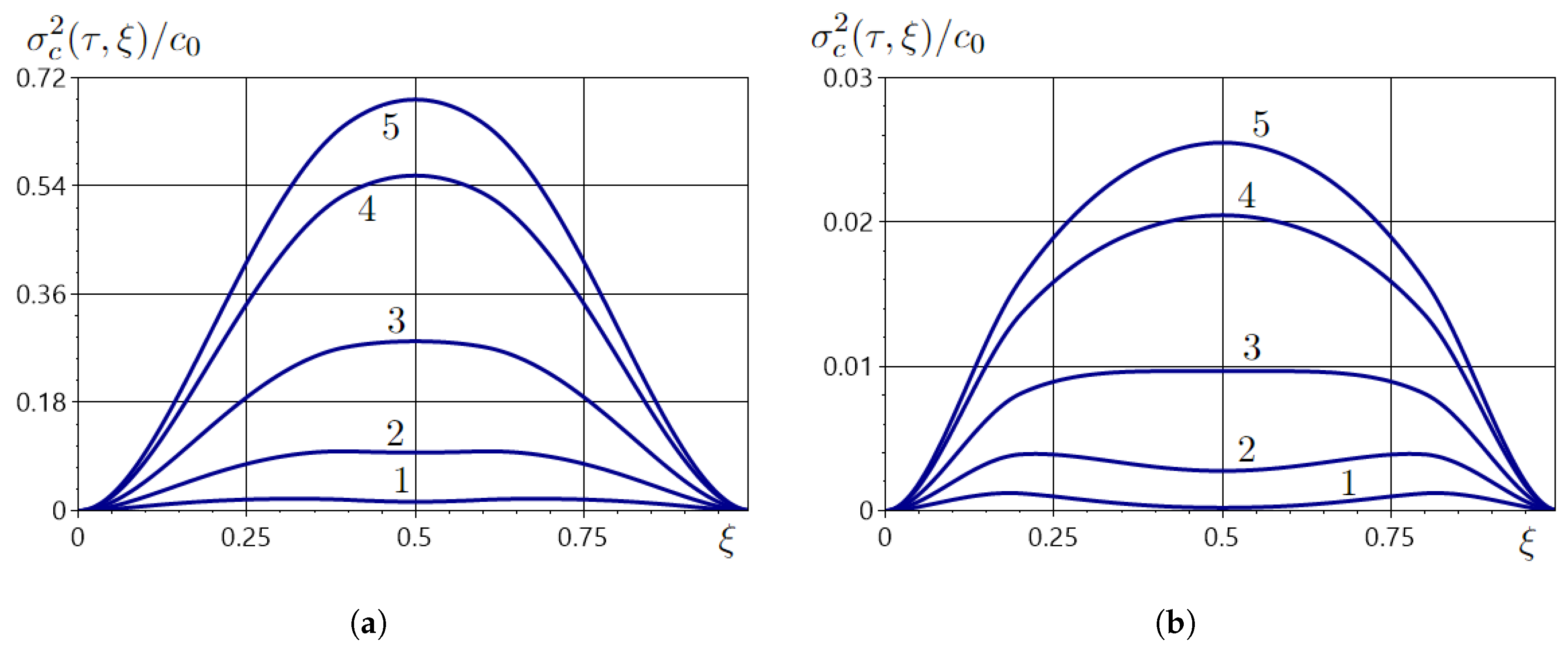
5.2. Second Moments of the Averaged Concentration Field

Let us find the variance ${\sigma }_C^2(t,\overrightarrow{r})$ of the impurity concentration field and the correlation (auto-correlation) function influenced by the point source system. The variance of the field ${\sigma }_C^2(t,\overrightarrow{r})$ is defined as [19]

$${\sigma }_C^2(t,\overrightarrow{r})=\langle C^2(t,\overrightarrow{r})\rangle -{\langle C(t,\overrightarrow{r})\rangle }^2.$$

(23)

For the averaged product of impurity concentration fields, the following expression holds:

$$\langle C(t_1,{\overrightarrow{r}}_1)C(t_2,{\overrightarrow{r}}_2)\rangle =\langle C(t_1,{\overrightarrow{r}}_1)\rangle \langle C(t_2,{\overrightarrow{r}}_2)\rangle +{\psi }_C(t_1,{\overrightarrow{r}}_1;t_2,{\overrightarrow{r}}_2),$$

(24)

where ${\psi }_C(t_1,{\overrightarrow{r}}_1;t_2,{\overrightarrow{r}}_2)$ is the correlation function (auto-correlation) of the concentration field $C(t,\overrightarrow{r})$ at the points $(t_1,{\overrightarrow{r}}_1)$ and $(t_2,{\overrightarrow{r}}_2)$.

Consequently, we obtain the correlation function of the field ${\psi }_C(t,\overrightarrow{r};t,\overrightarrow{r})$ at $(t,\overrightarrow{r})$

$${\psi }_C(t,\overrightarrow{r};t,\overrightarrow{r})=\langle C^2(t,\overrightarrow{r})\rangle -\langle C(t,\overrightarrow{r})\rangle \langle C(t,\overrightarrow{r})\rangle .$$

(25)

Then, the average of the square of the field can be expressed as

$$\langle C^2(t,\overrightarrow{r})\rangle =\langle C(t,\overrightarrow{r})C(t,\overrightarrow{r})\rangle =\langle C(t,\overrightarrow{r})\rangle \langle C(t,\overrightarrow{r})\rangle +{\psi }_C(t,\overrightarrow{r};t,\overrightarrow{r}).$$

(26)

Now, if we find the correlation function of the impurity particle concentration field ${\psi }_C(t,\overrightarrow{r};t,\overrightarrow{r})$ at the point $(t,\overrightarrow{r})$, we can then determine the variance of the field within the body.

Substitute the expressions for $C(t,\overrightarrow{r})$ (6) and $\langle C(t,\overrightarrow{r})\rangle$ (20) into Formula (25). First, we express $\langle C^2(t,z)\rangle$

$$\begin{array}{cc}\hfill \langle C^2(t,\overrightarrow{r})\rangle & ={\left(C^h(t,\overrightarrow{r})\right)}^2+2C^h(t,\overrightarrow{r})\hfill \\ \hfill & \times 〈\sum _{i=1}^n{\omega }_i{\int }_0^t{\int \int \int }_{\left(V\right)}G(t,t^{\prime },\overrightarrow{r},{\overrightarrow{r}}^{\prime })\delta ({\overrightarrow{r}}^{\prime }-{\widehat{\overrightarrow{r}}}_i)d^3{\overrightarrow{r}}^{\prime }d{t}^{\prime }〉\hfill \\ \hfill & +\sum _{i=1}^n\sum _{k=1}^n{\omega }_i{\omega }_k{\int }_0^t{\int \int \int }_{\left(V\right)}{\int }_0^t{\int \int \int }_{\left(V\right)}G(t,t^{\prime },\overrightarrow{r},{\overrightarrow{r}}^{\prime })\hfill \\ \hfill & \times G(t,t^{″},\overrightarrow{r},{\overrightarrow{r}}^{″})\langle \delta ({\overrightarrow{r}}^{\prime }-{\widehat{\overrightarrow{r}}}_i)\delta ({\overrightarrow{r}}^{″}-{\widehat{\overrightarrow{r}}}_k)\rangle d^3{\overrightarrow{r}}^{\prime }d{t}^{\prime }{d}^3{\overrightarrow{r}}^{″}d{t}^{″}.\hfill \end{array}$$

(27)

Taking into account Expression (27), the variance of the field can be represented as

$$\begin{array}{cc}\hfill {\sigma }_C^2(t,\overrightarrow{r})& =-{\langle C(t,\overrightarrow{r})\rangle }^2+{\left(C^h(t,\overrightarrow{r})\right)}^2+2C^h(t,\overrightarrow{r})\hfill \\ \hfill & \times 〈\sum _{i=1}^n{\omega }_i{\int }_0^t{\int \int \int }_{\left(V\right)}G(t,t^{\prime },\overrightarrow{r},{\overrightarrow{r}}^{\prime })\delta ({\overrightarrow{r}}^{\prime }-{\widehat{\overrightarrow{r}}}_i)d^3{\overrightarrow{r}}^{\prime }d{t}^{\prime }〉\hfill \\ \hfill & +\sum _{i=1}^n\sum _{k=1}^n{\omega }_i{\omega }_k{\int }_0^t{\int \int \int }_{\left(V\right)}{\int }_0^t{\int \int \int }_{\left(V\right)}G(t,t^{\prime },\overrightarrow{r},{\overrightarrow{r}}^{\prime })\hfill \\ \hfill & \times G(t,t^{″},\overrightarrow{r},{\overrightarrow{r}}^{″})\langle \delta ({\overrightarrow{r}}^{\prime }-{\widehat{\overrightarrow{r}}}_i)\delta ({\overrightarrow{r}}^{″}-{\widehat{\overrightarrow{r}}}_k)\rangle d^3{\overrightarrow{r}}^{\prime }d{t}^{\prime }{d}^3{\overrightarrow{r}}^{″}d{t}^{″}\hfill \end{array}$$

(28)

Allow for the system of n random point sources with a uniform distribution over the interval $[{\overline{z}}_1,{\overline{z}}_2]$, take into consideration the expression for the homogeneous concentration (10), substitute the Green function (15) into (28), and account for Expression (19) and the relation

$$\langle \delta ({\overrightarrow{r}}^{\prime }-{\widehat{\overrightarrow{r}}}_i)\delta ({\overrightarrow{r}}^{″}-{\widehat{\overrightarrow{r}}}_k)\rangle ={\displaystyle \frac{1}{4{\pi }^2{n}^2{({\overline{z}}_2-{\overline{z}}_1)}^2}}.$$

(29)

Finally, we obtain

$$\begin{array}{cc}\hfill {\sigma }_C^2(t,\overrightarrow{r})& ={\displaystyle \frac{4{\Omega }^2}{d^2{z}_0^2{n}^2{({\overline{z}}_2-{\overline{z}}_1)}^2}}\left({\left[\sum _{k=1}^{\infty }{\displaystyle \frac{1-{(-1)}^k}{z_k^3}}\left[1-e^{-d{z}_k^{2}t/\rho }\right]sin\left(z_{k}z\right)\right]}^2\right.\hfill \\ \hfill & -\left.{\left[\sum _{k=1}^{\infty }{S}_{12}\left(z_k\right)\left[1-e^{-d{z}_k^{2}t/\rho }\right]sin\left(z_{k}z\right)\right]}^2\right).\hfill \end{array}$$

(30)

Similarly, we defer the computational expression for the correlation function of the concentration field of the impurity substance, which diffuses in the strip under the influence of the system of random point sources, using the relation (28). We have

$${\psi }_C(t_1,{\overrightarrow{r}}_1,t_2,{\overrightarrow{r}}_2)={\displaystyle \frac{4{\Omega }^2}{d^2{z}_0^2{n}^2}}{\displaystyle \frac{1}{{({\overline{z}}_2-{\overline{z}}_1)}^2}}\sum _{k=1}^{\infty }\sum _{m=1}^{\infty }{A}_{km}{E}_k(t_1,z_1)E_m(t_2,z_2),$$

(31)

where

$$A_{km}=\left[{\displaystyle \frac{1}{z_k^3{z}_m^3}}(1-{(-1)}^k)(1-{(-1)}^m)-S_{12}\left(z_k\right)S_{12}\left(z_m\right)\right],$$

(32)

$$E_k(t,z)=\left[1-e^{-d{z}_k^{2}t/\rho }\right]sin\left(z_{k}z\right),k=n,m.$$

(33)

Note that the correlation function ${\psi }_c(t_1,{\overrightarrow{r}}_1;t_2,{\overrightarrow{r}}_2)$ is directly proportional to the square of the total power of the point sources in the system and inversely proportional to the square of the number of sources.

If the sources have the same power, then Formula (31) simplifies to

$${\psi }_C(t_1,{\overrightarrow{r}}_1;t_2,{\overrightarrow{r}}_2)={\displaystyle \frac{4{\omega }^2}{d^2{z}_0^2}}{\displaystyle \frac{1}{{({\overline{z}}_2-{\overline{z}}_1)}^2}}\sum _{k=1}^{\infty }\sum _{m=1}^{\infty }{A}_{km}{E}_k(t_1,z_1)E_m(t_2,z_2).$$

(34)

In the case where the sources are of equal power, as well as in the general case (31), the correlation function is inversely proportional to the squared length of the internal interval of source action $[{\overline{z}}_1,{\overline{z}}_2]$.

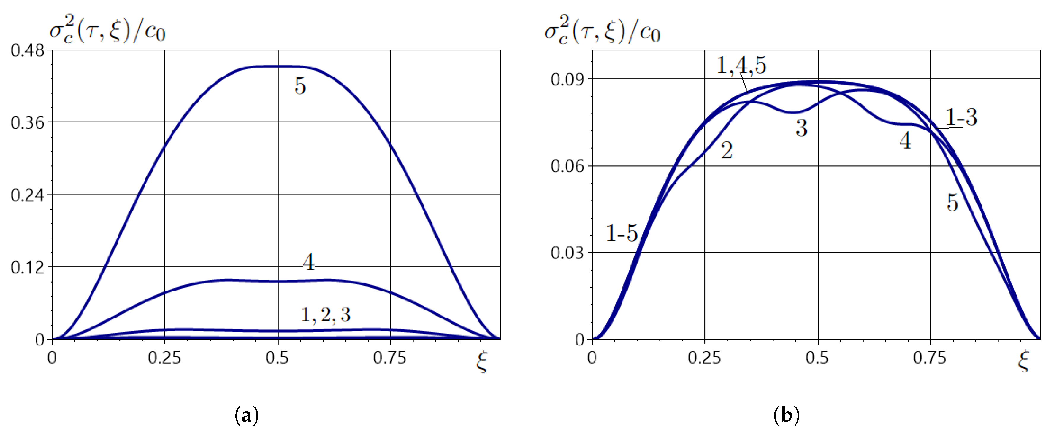
5.3. Numerical Analysis of the Variance and Correlation Function of the Concentration Field

Figure 8, Figure 9 and Figure 10 illustrate characteristic distributions of the variance of the concentration field of the impurity substance in the strip under the influence of the system of point sources. Calculations were performed using dimensionless variables (22) with the same base parameter values. Figure 8 shows the variance at different dimensionless times $\tau =0.02,0.05,0.1,0.2,0.3$ (lines 1–5) for the following intervals of point source action: $[{\overline{\xi }}_1,{\overline{\xi }}_2]=[0.4,0.6]$ (a) and $[{\overline{\xi }}_1,{\overline{\xi }}_2]=[0.2,0.8]$ (b).

Presented in

Table 1. Maximum of the variance and the points at which this maximum is achieved.

$\mathit{\tau }$	${\mathit{\xi }}_1,{\mathit{\xi }}_2=[0.4,0.6]$		${\mathit{\xi }}_1,{\mathit{\xi }}_2=[0.2,0.8]$
	${\mathit{\xi }}_{\mathbf{1}},{\mathit{\xi }}_{\mathbf{2}}$	${\mathbf{max}}_{\mathit{\xi }\mathbf{\in }\mathbf{[}\mathbf{0},{\mathit{\xi }}_{\mathbf{1}}\mathbf{]}}\mathit{\sigma }$	${\mathit{\xi }}_{\mathbf{1}},{\mathit{\xi }}_{\mathbf{2}}$	${\mathbf{max}}_{\mathit{\xi }\mathbf{\in }\mathbf{[}\mathbf{0},{\mathit{\xi }}_{\mathbf{1}}\mathbf{]}}\mathit{\sigma }$
0.02	0.3237, 0.6763	0.0198	0.1850, 0.8150	0.0012
0.05	0.3931, 0.6069	0.0987	0.2197, 0.7803	0.0039
0.1	0.5	0.2817	0.4335, 0.5665	0.0097
0.2	0.5	0.5574	0.5	0.0205
0.3	0.5	0.6838	0.5	0.0225

are the maximum of the variance $\underset{\xi \in [0,{\xi }_0]}{max}\sigma (\tau ,\xi )$ and the point ${\xi }_{max}$ at which this maximum is achieved, for the data illustrated in Figure 8.

Figure 9 shows the variance ${\sigma }_C^2$ under the action of the system with one source with a significantly amount of power. More specifically, Figure 9a is plotted for $[{\overline{\xi }}_1,{\overline{\xi }}_2]=[0.4,0.6]$, and Figure 9b for $[{\overline{\xi }}_1,{\overline{\xi }}_2]=[0,{\xi }_0]$. Here, line 1 corresponds to the system $\{1,1,1,1,40\}$, line 2 to $\{1,1,1,1,30\}$, line 3 to $\{1,1,1,1,20\}$, line 4 to $\{1,1,1,1,10\}$, and line 5 to $\{1,1,1,1,1\}$.

The variance values increase significantly with the duration of the diffusion process (Figure 8). That is observed when the interval of point source action is located in the middle of the strip and when this interval nearly covers the entire region of the body. Specifically, as $\tau$ increases from $0.02$ to $0.3$, the maximum values of the variance increase by an order of magnitude (Table 1): $\underset{\xi \in [0,{\xi }_0]}{max}{\sigma }_c^2(\tau ,\xi ){|}_{\tau =0.3}/\underset{\xi \in [0,{\xi }_0]}{max}{\sigma }_c^2(\tau ,\xi ){|}_{\tau =0.02}\approx 34.5$.

Note that the number of sources, provided they have the same average power, does not affect the variance. A change in the value of $\Omega$ leads to a change in ${\sigma }_C^2$ (Figure 9).

If there is a dominant power source within the system, the behavior of the variance function remains unchanged. However, the power of such a source significantly influences the value of ${\sigma }_C^2$ (Figure 9). For example, as ${\omega }_{max}$ increases from 10 to 40, the maximum values of the variance grow by an order of magnitude (Table 1):

$$\underset{\xi \in [0,{\xi }_0]}{max}{\sigma }_c^2(\tau ,\xi ){|}_{\begin{array}{c}[{\overline{\xi }}_1,{\overline{\xi }}_2]=[0.4,0.6],\\ {\omega }_{max}=40\end{array}}/\underset{\xi \in [0,{\xi }_0]}{max}{\sigma }_c^2(\tau ,\xi ){|}_{\begin{array}{c}[{\overline{\xi }}_1,{\overline{\xi }}_2]=[0.4,0.6],\\ {\omega }_{max}=10\end{array}}\approx 9.9;$$

(35)

$$\underset{\xi \in [0,{\xi }_0]}{max}{\sigma }_c^2(\tau ,\xi ){|}_{\begin{array}{c}[{\overline{\xi }}_1,{\overline{\xi }}_2]=[0,1],\\ {\omega }_{max}=40\end{array}}/\underset{\xi \in [0,{\xi }_0]}{max}{\sigma }_c^2(\tau ,\xi ){|}_{\begin{array}{c}[{\overline{\xi }}_1,{\overline{\xi }}_2]=[0,1],\\ {\omega }_{max}=10\end{array}}\approx 9.9.$$

(36)

Figure 10 shows the variance of the concentration field (a) for different lengths of the interval where the point sources act $[{\overline{\xi }}_1,{\overline{\xi }}_2]=[0.1,0.9];[0.2,0.8];[0.3,0.7];[0.4,0.6];[0.45,0.55]$ (lines 1–5) and (b) for different positions $[{\overline{\xi }}_1,{\overline{\xi }}_2]=[0.0,0.1];[0.2,0.3];[0.4,0.5];[0.6,0.7];$$[0.8,0.9]$ of this interval (lines 1–5).

From the start of the process of mass transfer, two local maxima of the variance are observed, which become less distinct as the interval $[{\overline{\xi }}_1,{\overline{\xi }}_2]$ enlarges (curves 1–5, Figure 10a). For $[{\overline{\xi }}_1,{\overline{\xi }}_2]=[0.4,0.5]$, there is only one maximum of ${\sigma }_C^2$ at the point ${\xi }_{max}=0.5$ (curve 3 in Figure 10b).

Note that the thinner the interval of point source action, the higher the variance values across the entire region of the body. If this interval is centered within the body, then despite different concentration values at the upper and lower boundaries of the strip, the variance is nearly a symmetric function (Figure 8, Figure 9 and Figure 10a). If the interval $[{\overline{\xi }}_1,{\overline{\xi }}_2]$ is located close to the center of the strip, a loss of monotonicity in the variance is also observed in the segments $\xi \in [0,0.5)$ and $\xi \in (0.5,1]$ (curves 2–4, Figure 10b). In the case when the interval shifts towards one of the strip boundaries, the symmetry of the function ${\sigma }_C^2(t,z)$ is lost.

It should also be noted that if the interval $[{\overline{\xi }}_1,{\overline{\xi }}_2]$ is located in the upper half of the strip, the maximum of variance is reached in the lower half of the body (curves 2, 3, Figure 10b). On the other hand, if $[{\overline{\xi }}_1,{\overline{\xi }}_2]$ is located in the lower half of the strip, the maximum variance is reached in the upper half of the body (curves 4, 5, Figure 10b).

Figure 11, Figure 12, Figure 13, Figure 14, Figure 15, Figure 16, Figure 17 and Figure 18 show the characteristic surfaces formed by the correlation function ${\psi }_C({\tau }_1,{\xi }_1,{\tau }_2,{\xi }_2)$ (a) and the corresponding 2D plots (b). Calculations are carried out for the system of three mass sources with equal power. For small times ${\tau }_1=0.05$ and ${\tau }_2=0.06$, 3D and 2D plots of the correlation function are displayed for the following intervals of point source action: $[{\overline{\xi }}_1,{\overline{\xi }}_2]=[0.4,0.6]$ in Figure 11, $[{\overline{\xi }}_1,{\overline{\xi }}_2]=[0.1,0.3]$ in Figure 12, $[{\overline{\xi }}_1,{\overline{\xi }}_2]=[0.7,0.9]$ in Figure 13, and $[{\overline{\xi }}_1,{\overline{\xi }}_2]=[0.2,0.8]$ in Figure 14.

In Figure 15, Figure 16, Figure 17 and Figure 18, we demonstrate 3D and 2D graphs of the correlation function ${\psi }_c({\tau }_1,{\xi }_1,{\tau }_2,{\xi }_2)$ for ${\tau }_1=0.5$ and ${\tau }_2=0.06$ for the intervals $[{\overline{\xi }}_1,{\overline{\xi }}_2]=[0.2,0.8]$ (Figure 15 and Figure 16), for $[{\overline{\xi }}_1,{\overline{\xi }}_2]=[0.2,0.3]$ (Figure 17), and for $[{\overline{\xi }}_1,{\overline{\xi }}_2]=[0.8,0.9]$ (Figure 18).

In most cases, the characteristic surfaces formed by the correlation function $\psi ({\tau }_1,{\xi }_1,{\tau }_2,{\xi }_2)$ are nearly symmetric (Figure 11 and Figure 14, Figure 15, Figure 16, Figure 17 and Figure 18). However, for small times and when the interval is located in the vicinity of one of the strip boundaries, $\psi ({\tau }_1,{\xi }_1,{\tau }_2,{\xi }_2)$ is not symmetric (Figure 12 and Figure 13). Symmetry in the surface emerges as time grows (Figure 17 and Figure 18).

For small values of ${\tau }_1$ and ${\tau }_2$ (Figure 11, Figure 12 and Figure 13), the function $\psi ({\tau }_1,{\xi }_1,{\tau }_2,{\xi }_2)$ reaches its highest values in the middle of the strip. The closer the interval of point source action $[{\overline{\xi }}_1,{\overline{\xi }}_2]$ is to the strip’s surface $\xi =0$, the slower the decline of the correlation function, while the maximum values of $\psi ({\tau }_1,{\xi }_1,{\tau }_2,{\xi }_2)$ remain constant. If the sub-strip $[{\overline{\xi }}_1,{\overline{\xi }}_2]$ increases, the values of the correlation function in the middle of the strip increase.

Additionally, the longer the time interval $[{\tau }_1,{\tau }_2]$, the more likely two local maxima of the correlation function will arise (Figure 14 and Figure 15). Shifting the sub-strip $[{\overline{\xi }}_1,{\overline{\xi }}_2]$ closer to the boundary $\xi =0$ or $\xi ={\xi }_0$ leads to a more symmetric shape of the surface $\psi ({\tau }_1,{\xi }_1,{\tau }_2,{\xi }_2)$.

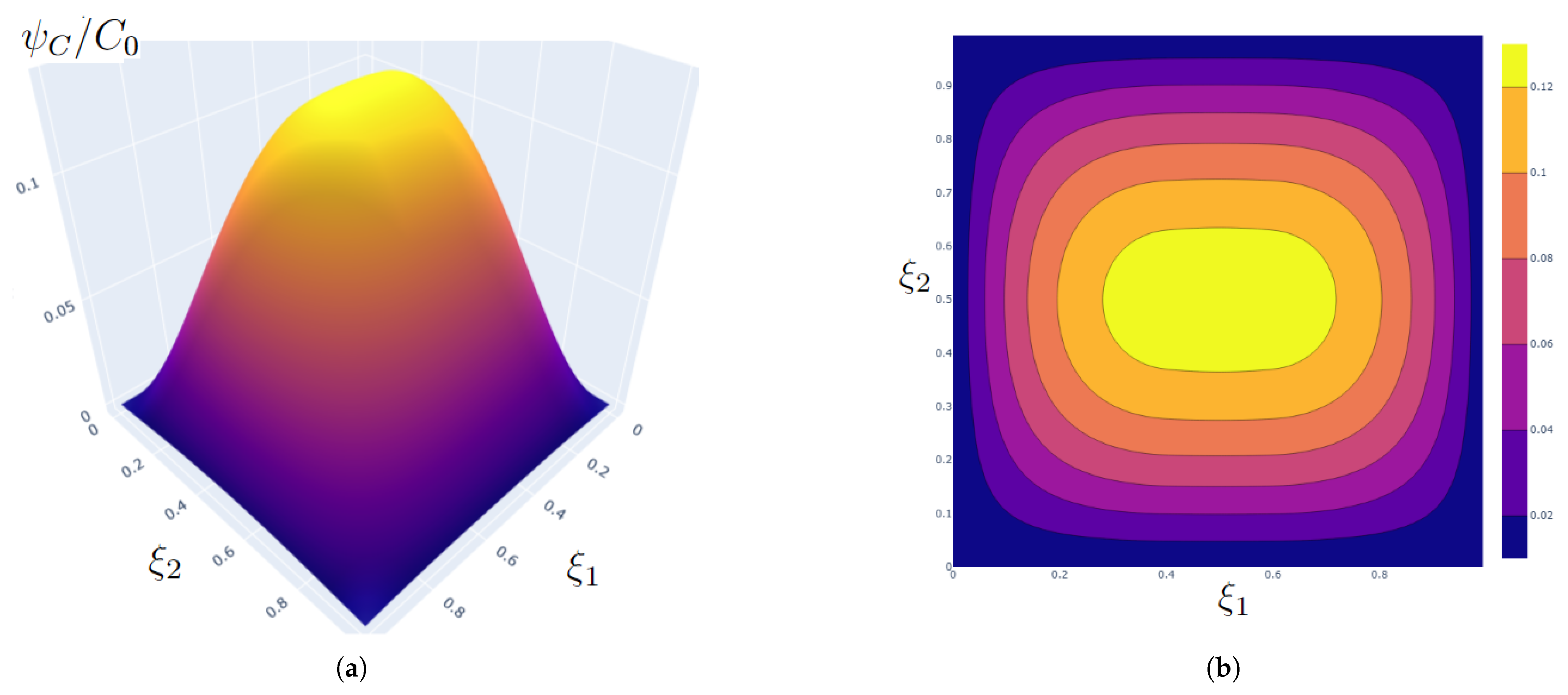
5.4. Correlation Coefficient

The correlation coefficient of the concentration field $K_C(t_1,z_1;t_2,z_2)$, which determines the numerical measure of dependence of the field values at points $(t_1,z_1)$ and $(t_2,z_2)$, is defined by Expression [19]:

$$K_C(t_1,z_1;t_2,z_2)={\displaystyle \frac{{\psi }_C(t_1,z_1;t_2,z_2)}{\sqrt{{\sigma }_C^2(t_1,z_1){\sigma }_C^2(t_2,z_2)}}}.$$

(37)

We substitute the expressions for the correlation function ${\psi }_C$ (31) and the variance ${\sigma }_C^2$ (30) into Formula (37). Then, we have

$$\begin{array}{cc}\hfill & K_C(t_1,z_1;t_2,z_2)=\hfill \\ \hfill & {\displaystyle \frac{{\sum }_{k=1}^{\infty }{\sum }_{m=1}^{\infty }{A}_{km}{E}_k(t_1,z_1)E_m(t_2,z_2)}{\sqrt{{\sum }_{k=1}^{\infty }{\sum }_{m=1}^{\infty }{B}_{km}^{-}{B}_{km}^{+}{\overline{E}}_{km}(t_1,z_1){\sum }_{l=1}^{\infty }{\sum }_{p=1}^{\infty }{B}_{lp}^{-}{B}_{lp}^{+}{\overline{E}}_{lp}(t_2,z_2)}}},\hfill \end{array}$$

(38)

where

$$\begin{array}{c}{\overline{E}}_{ij}(t,z)=E_i(t,z)E_j(t,z);i=k,l;j=m,p,\\ B_{km}^{\pm }=\left[1-{(-1)}^k\right]/z_k^3\pm S_{12}\left(z_m\right).\end{array}$$

(39)

From the obtained Formula (38), it follows that the correlation coefficient does not depend on the power of the point sources or their quantity.

The values of the correlation coefficient of the concentration field at different points $(t_1,z_1)$ and $(t_2,z_2)$ for intervals of point sources action $[{\overline{\xi }}_1,{\overline{\xi }}_2]=[0.4,0.6]$ and $[{\overline{\xi }}_1,{\overline{\xi }}_2]=[0.2,0.8]$ are presented in

Table 2. Correlation coefficient of the concentration field for interval of point sources action $[{\overline{\xi }}_1,{\overline{\xi }}_2]=[0.4,0.6]$ and $[{\overline{\xi }}_1,{\overline{\xi }}_2]=[0.2,0.8]$.

$[{\overline{\mathit{\xi }}}_1,{\overline{\mathit{\xi }}}_2]=[0.4,0.6]$					$[{\overline{\mathit{\xi }}}_1,{\overline{\mathit{\xi }}}_2]=[0.2,0.8]$
${\mathit{\xi }}_{\mathbf{1}}$	${\mathit{\xi }}_{\mathbf{2}}$	${\mathit{\tau }}_{\mathbf{1}}$	${\mathit{\tau }}_{\mathbf{2}}$	${\mathit{K}}_{\mathit{C}}$	${\mathit{\xi }}_{\mathbf{1}}$	${\mathit{\xi }}_{\mathbf{2}}$	${\mathit{\tau }}_{\mathbf{1}}$	${\mathit{\tau }}_{\mathbf{2}}$	${\mathit{K}}_{\mathit{C}}$
0.1416	0.0620	0.5	0.45	0.8975	0.1416	0.0620	0.5	0.45	0.8013
0.1416	0.4956	0.5	0.45	0.8942	0.1416	0.4956	0.5	0.45	0.7532
0.0177	0.5044	0.5	0.45	0.8014	0.0177	0.5044	0.5	0.45	0.6137
0.7234	0.7123	0.5	0.45	0.9748	0.7234	0.7123	0.5	0.45	0.9647
0.1681	0.1062	0.05	0.06	0.8199	0.1681	0.1062	0.05	0.06	0.7076
0.1504	0.5044	0.05	0.06	0.7925	0.1504	0.5044	0.05	0.06	0.6069
0.0880	0.4956	0.05	0.06	0.7133	0.0880	0.4956	0.05	0.06	0.5121
0.2312	0.8612	0.05	0.06	0.8973	0.2312	0.8612	0.05	0.06	0.8661

.

Note that the correlation coefficient reaches its highest values when points ${\xi }_1$ and ${\xi }_2$ are located in the middle of the strip both for $[{\overline{\xi }}_1,{\overline{\xi }}_2]=[0.4,0.6]$ and for $[{\overline{\xi }}_1,{\overline{\xi }}_2]=[0,1]$ (Table 2), i.e., here, the relationship between the concentration field at points $\xi ={\xi }_1$ and $\xi ={\xi }_2$ is the strongest. The greater the distance from $\xi ={\xi }_1$ to $\xi ={\xi }_2$, the smaller values the correlation coefficient takes on.

The relationship between the concentration field values at $({\tau }_1,{\xi }_1)$ and $({\tau }_2,{\xi }_2)$ is substantially non-linear (Table 2). When both points ${\xi }_1$ and ${\xi }_2$ shift to the lower boundary of the strip, then this relationship tends to linear.

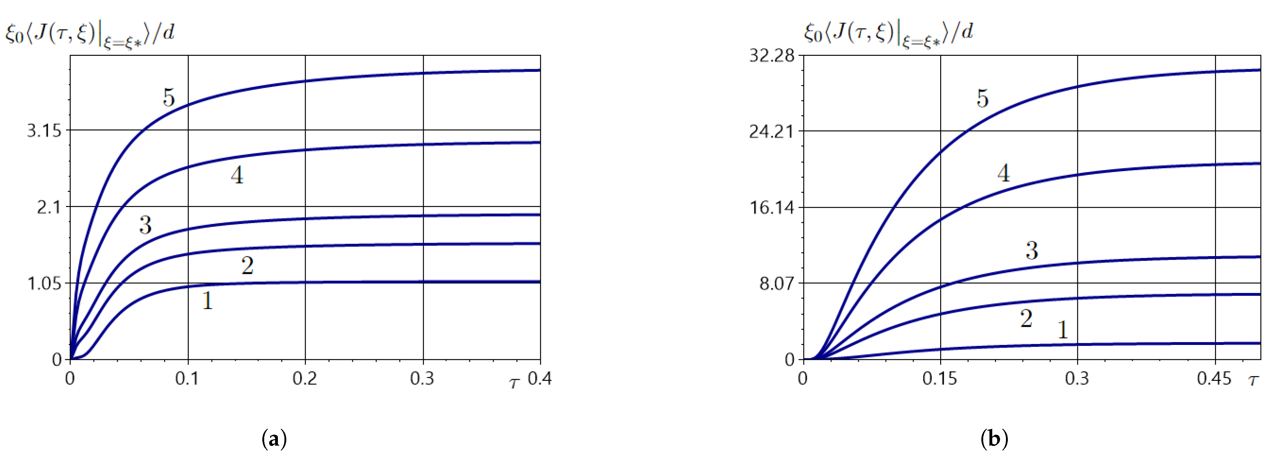
5.5. Diffusive Fluxes Affected by the System of Random Point Sources of Mass

In general, the diffusive flux $\overrightarrow{J}(t,\overrightarrow{r})$ is determined by Fick’s first law [20]

$$\overrightarrow{J}(t,\overrightarrow{r})=-d\overrightarrow{\nabla }C(t,\overrightarrow{r}).$$

(40)

The formal expression for the random mass flux $J(t,\overrightarrow{r})$ passing through section $\overrightarrow{r}={\overrightarrow{r}}_{*}$ is found by differentiating Formula (6) and taking into account (10). Then, we have

$$\begin{array}{cc}\hfill & \overrightarrow{J}(t,\overrightarrow{r}){|}_{\overrightarrow{r}={\overrightarrow{r}}_{*}}={\overrightarrow{J}}_h(t,\overrightarrow{r}){|}_{\overrightarrow{r}={\overrightarrow{r}}_{*}}\hfill \\ \hfill & -d\overrightarrow{\nabla }\sum _{i=1}^n{\omega }_i{\int }_0^t{\int \int \int }_{\left(V\right)}G(t,t^{\prime },\overrightarrow{r},{\overrightarrow{r}}^{\prime })\delta ({\overrightarrow{r}}^{\prime }-{\widehat{\overrightarrow{r}}}_i)d^3{\overrightarrow{r}}^{\prime }d{t}^{\prime }{|}_{\overrightarrow{r}={\overrightarrow{r}}_{*}},\hfill \end{array}$$

(41)

where ${\overrightarrow{r}}_{*}=(x,y,z_{*})$ and ${\overrightarrow{J}}_h(t,\overrightarrow{r})$ is the diffusive flux in the strip without internal point sources, specifically

$$\begin{array}{cc}\hfill {\overrightarrow{J}}_h(t,\overrightarrow{r}){|}_{z=z_{*}}& ={\displaystyle \frac{d}{z_0}}[C_0-C_{*}\hfill \\ \hfill & +{\displaystyle \frac{2}{\rho }}\sum _{k=1}^{\infty }\left(C_0+{(-1)}^{k+1}{C}_{*}\right)e^{-d{z}_k^{2}t/\rho }cos\left(z_k{z}_{*}\right)].\hfill \end{array}$$

(42)

In particular, the flux ${\overrightarrow{J}}_h(t,\overrightarrow{r})$ through the lower boundary of the strip $z=z_0$ has the form

$${\overrightarrow{J}}_h(t,\overrightarrow{r}){|}_{z=z_0}={\displaystyle \frac{d}{z_0}}\left[C_0-C_{*}+{\displaystyle \frac{2}{\rho }}\sum _{k=1}^{\infty }\left[{(-1)}^k{C}_0-C_{*}\right]e^{-d{z}_k^{2}t/\rho }\right].$$

(43)

Now, we obtain the formula for the flux taking into account the influence of the system of point sources. Substituting Green’s function (15) into Formula (41), we obtain

$$\begin{array}{cc}\hfill & \overrightarrow{J}(t,\overrightarrow{r}){|}_{\overrightarrow{r}={\overrightarrow{r}}_{*}}={\overrightarrow{J}}_h(t,\overrightarrow{r}){|}_{\overrightarrow{r}={\overrightarrow{r}}_{*}}-{\displaystyle \frac{1}{z_0}}\overrightarrow{\nabla }\sum _{i=1}^n{\omega }_i\hfill \\ \hfill & \times {\int }_0^t{\int \int \int }_{\left(V\right)}{\displaystyle \frac{\theta (t-t^{\prime })}{t-t^{\prime }}}exp\left\{-{\displaystyle \frac{\rho }{4d}}{\displaystyle \frac{{(x-x^{\prime })}^2+{(y-y^{\prime })}^2}{t-t^{\prime }}}\right\}\hfill \\ \hfill & \times \sum _{k=1}^{\infty }{e}^{-d{z}_k^2(t-t^{\prime })/\rho }sin\left(z_k{z}^{\prime }\right)sin\left(z_{k}z\right)\delta ({\overrightarrow{r}}^{\prime }-{\widehat{\overrightarrow{r}}}_i)d^3{\overrightarrow{r}}^{\prime }d{t}^{\prime }{|}_{\overrightarrow{r}={\overrightarrow{r}}_{*}}.\hfill \end{array}$$

(44)

Next, we average the diffusive flux (44) over the random point source coordinates ${\widehat{\overrightarrow{r}}}_i$ with uniform distribution (17) over the strip $[{\overline{z}}_1,{\overline{z}}_2]\subseteq [0,z_0]$. We factor in that $J_h$ is a deterministic function, i.e., $\langle J_h\rangle =J_h$. We then obtain the computational formula for the averaged diffusive flux through the surface $z=z_{*}$

$$\begin{array}{cc}\hfill 〈\overrightarrow{J}(t,\overrightarrow{r}){|}_{\overrightarrow{r}={\overrightarrow{r}}_{*}}〉& ={\displaystyle \frac{d}{z_0}}\left[C_0-C_{*}\right]\hfill \\ \hfill & +{\displaystyle \frac{d}{z_0}}{\displaystyle \frac{2}{\rho }}\sum _{k=1}^{\infty }\left(C_0+{(-1)}^{k+1}{C}_{*}\right)e^{-d{z}_k^{2}t/\rho }cos\left(z_k{z}_{*}\right)\hfill \\ \hfill & -{\displaystyle \frac{2\Omega }{z_{0}n({\overline{z}}_2-{\overline{z}}_1)}}\sum _{k=1}^{\infty }{\displaystyle \frac{1-e^{-d{z}_k^{2}t/\rho }}{z_k^2}}\hfill \\ \hfill & \times cos\left(z_k{z}_{*}\right)[cos\left(z_k{\overline{z}}_1\right)-cos\left(z_k{\overline{z}}_2\right)].\hfill \end{array}$$

(45)

In particular, the flux passing through the lower boundary of the strip takes the form

$$\begin{array}{cc}\hfill 〈\overrightarrow{J}(t,\overrightarrow{r}){|}_{z=z_0}〉& ={\displaystyle \frac{d}{z_0}}\left[C_0-C_{*}+{\displaystyle \frac{2}{\rho }}\sum _{k=1}^{\infty }\left({(-1)}^k{C}_0-C_{*}\right)e^{-d{z}_k^{2}t/\rho }\right]\hfill \\ \hfill & -{\displaystyle \frac{2\Omega }{z_{0}n({\overline{z}}_2-{\overline{z}}_1)}}\sum _{k=1}^{\infty }{(-1)}^k{\displaystyle \frac{1-e^{-d{z}_k^{2}t/\rho }}{z_k^2}}\hfill \\ \hfill & [cos\left(z_k{\overline{z}}_1\right)-cos\left(z_k{\overline{z}}_2\right)].\hfill \end{array}$$

(46)

The characteristic behavior of the averaged diffusive fluxes in a strip of dimensionless width $z_0$ when the random sources composing the system are disposed uniformly is illustrated in Figure 19, Figure 20 and Figure 21. Expressions (42)–(46) are used for diffusive flux calculations. Here, the series were computed with an accuracy of ${10}^{-12}$.

Figure 19 features the graphs of the averaged fluxes $\langle J{|}_{z=z_{*}}\rangle$ influenced by the acting point sources and the diffusive fluxes $J_h{|}_{z=z_{*}}$ without the internal point sources across variant sections $z_{*}=0.55,0.6,1$ (curves 1–3 correspondingly). The solid lines of curves a represent $\langle J{|}_{x=x*}\rangle$, while the dashed lines of curves b represent $J_h(\tau ,z)$. The calculations in Figure 19a are carried out for the interval $[{\overline{z}}_1,{\overline{z}}_2]=[0.4,0.6]$, and in Figure 19b for the interval $[{\overline{z}}_1,{\overline{z}}_2]=[0.2,0.8]$.

Shown in Figure 20 is the typical behavior of averaged diffusive fluxes under the influence of the system consisting of three point sources of the same power for different total powers $\Omega$. Curve 1 represents the system $\{1.5,1.5,1.5\}$; curve 2—$\{3,3,3\}$; curve 3—$\{6,6,6\}$; curve 4—$\{12,12,12\}$; and curve 5—$\{60,60,60\}$. Figure 21 demonstrates the plots of flux $z_0\langle J(\tau ,z){|}_{z=z_{*}}\rangle /d$ for different point source quantities with the same $\Omega =18$, i.e., $\omega =0.3,1.5,4.5,9,18$ (curves 1–5). Here, Figure 21a is plotted for the fluxes through the section $z_{*}=0.51$ and Figure 21b is plotted for $z_{*}=1$.

It is important to highlight that the existence of random point sources in the system significantly affects the value of the averaged diffusive flux (45) but barely influences its behavior (Figure 19). For example, the flux values in the steady-state regime are higher the closer the section point is to the boundary $z=z_0$. When internal sources act in the system, there is a more rapid increase in flux $\langle J\rangle$ compared to $J_h$ for short time periods. In the absence of internal sources, the closer the section $z=z_{*}$ is to the lower boundary of the strip, the smaller the flux values are over the entire time interval. The value of the $J_h$ in the steady-state regime for different sections $z=z_{*}$ is the same (curves 1b–3b in Figure 19). Meanwhile, the value of the flux without the internal sources action is several times smaller than the value of the averaged flux.

Analyzing the impact of the thickness of the of the source action interval on the averaged flux, it is observed that the highest values are reached for small widths of the interval (curve 5, Figure 20a,b).

The closer the source action interval is to the body boundary at $z=0$ (Figure 21b), the smaller the values of the averaged diffusion flux through the lower boundary of the strip. When the interval $[{\overline{z}}_1,{\overline{z}}_2]$ is positioned in the proximity of the top boundary of the strip for sections $z=z_{*}$ in the middle of the body, the flux $\langle J\rangle$ is a monotonically increasing function (curve 1, Figure 21a). As the interval shifts away from the boundary $z=0$, the diffusive flux values increase (curve 2, Figure 21a).

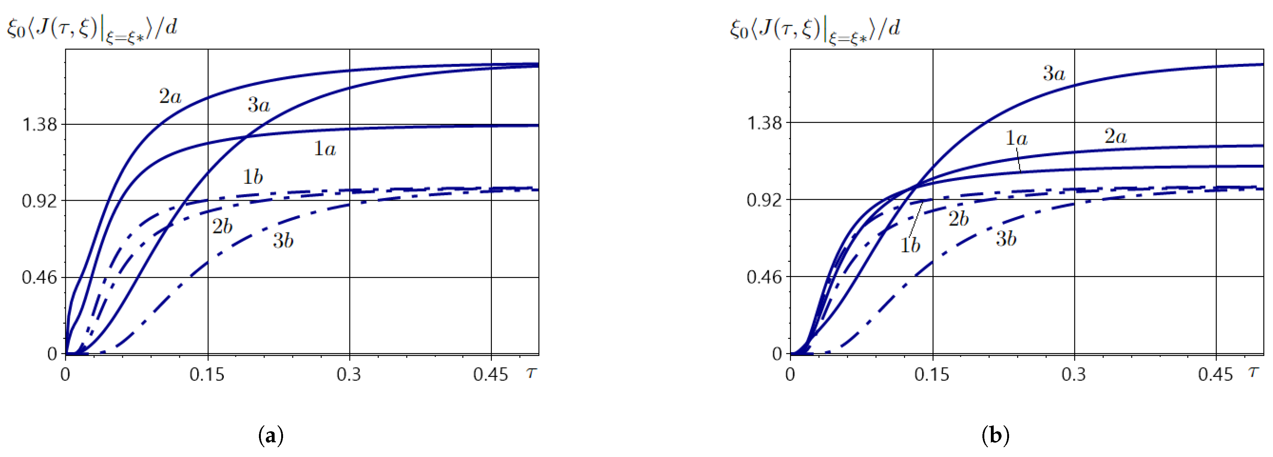
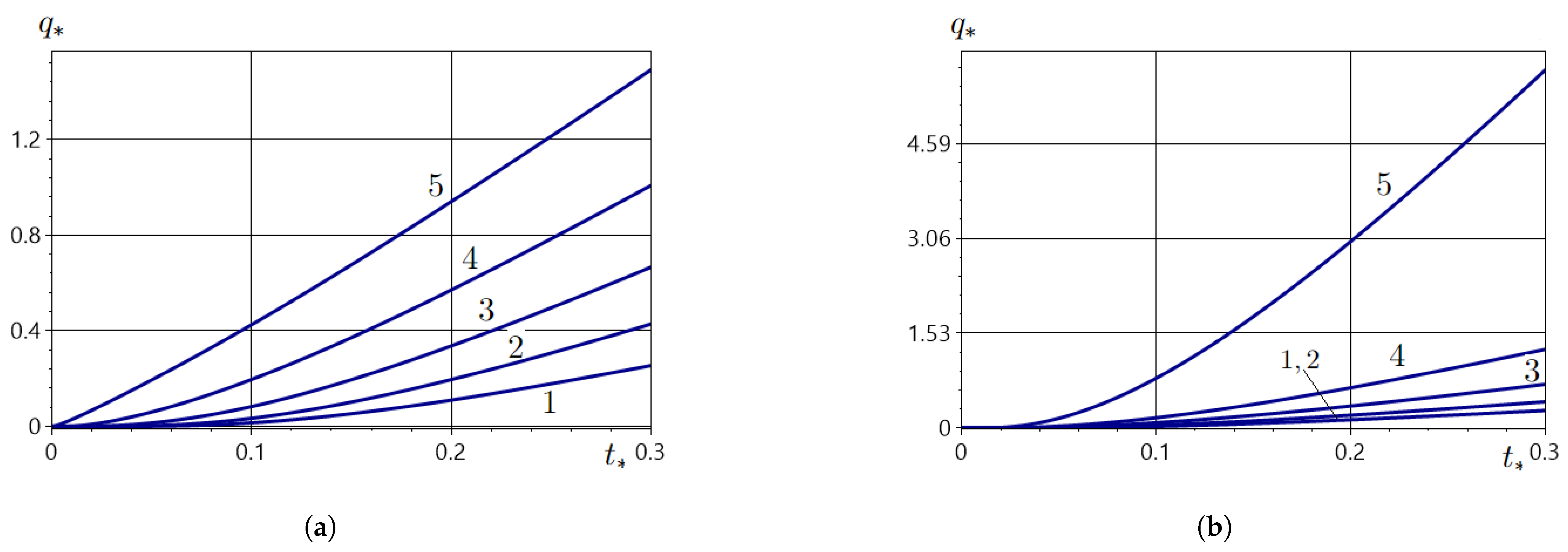
5.6. Amount of Substance Passed Through the Strip over Time $t_{*}$

Let us also find the amount of substance that has passed through the strip over the given time interval $t_{*}$, defined by the formula

$$q_{*}={\int }_0^{t_{*}}〈J(t,\overrightarrow{r}){|}_{z=z_0}〉dt.$$

(47)

Herewith, we use the calculating formulas for the averaged fluxes (45) and (46). Integrating these expressions over time, we obtain

$$\begin{array}{cc}\hfill q_{*}& ={\displaystyle \frac{t_{*}d}{z_0}}\left[C_0-C_{*}-{\displaystyle \frac{2\Omega }{dn({\overline{z}}_2-z_1)}}\sum _{k=1}^{\infty }{\displaystyle \frac{{(-1)}^k}{z_k^2}}\left[cos\left(z_k{\overline{z}}_1\right)-cos\left(z_k{\overline{z}}_2\right)\right]\right.\hfill \\ \hfill & +{\displaystyle \frac{2}{z_0}}\sum _{k=1}^{\infty }{\displaystyle \frac{{(-1)}^k}{z_k^2}}\left\{C_0+{(-1)}^{k+1}{C}_{*}+{\displaystyle \frac{\rho \Omega [cos\left(z_k{\overline{z}}_1\right)-cos\left(z_k{\overline{z}}_2\right)]}{dn({\overline{z}}_2-{\overline{z}}_1)z_k^2}}\right\}\hfill \\ & \left.\times \left(1-e^{-d{z}_k^2{t}_{*}/\rho }\right)\right].\hfill \end{array}$$

(48)

The asymptotic part of the amount of substance that has passed through the strip is directly proportional to the duration $t_{*}$ of the diffusion process. Graphs of the amount of impurity substance that has passed through the strip with dimensionless width $z_0$ when the point mass sources are distributed uniformly over a certain internal interval are presented in Figure 22. Figure 22a shows the graphs of $q_{*}$ for different positions of the point source action interval: $[{\overline{z}}_1,{\overline{z}}_2]=[0.1,0.2]$, $[{\overline{z}}_1,{\overline{z}}_2]=[0.3,0.4]$, $[{\overline{z}}_1,{\overline{z}}_2]=[0.5,0.6]$, $[{\overline{z}}_1,{\overline{z}}_2]=[0.7,0.8]$, $[{\overline{z}}_1,{\overline{z}}_2]=[0.9,1]$ (curves 1–5, respectively). Figure 22b presents the function $q_{*}$ for the system of three sources of equal power for different total power $\Omega =4.5,9,18,38,180$ (curves 1–5).

Note that the position of the action interval of the system of random point mass sources substantially changes the amount of substance $q_{*}$ that passes through the lower surface of the strip over time $t_{*}$. The closer this interval is located to the lower boundary $z=z_0$, the greater and the more rapid the increase in $q_{*}$ over time (Figure 22a). Value $q_{*}$ grows larger as the total power $\Omega$ increases (Figure 22b).

6. Discussion

The findings of the investigation offer a comprehensive framework for understanding impurity diffusion in media influenced by random point mass sources. A critical aspect of this research is the explicit consideration of the statistical properties of these sources, which allows for the derivation of averaged characteristics of the diffusion process. This approach bridges the gap between purely deterministic models and more complex probabilistic scenarios, offering a significant advantage in applications where the exact location and intensities of sources are uncertain.

It has been shown that the presence of a system of point mass sources within the body increases both the averaged concentration of the migrating substance and the averaged diffusive flux. Specifically, a characteristic increase in the averaged field of concentration is seen within the interval of the source action. It should be highlighted that the averaged concentration within the interval is influenced only by the mean power of the system’s sources and not influenced by the power of any specific source. Regarding the flux function, it has been established that the closer the interval where the source system acts to the lower surface of the strip and/or the section plane through which the flux is measured, the greater the impurity flux values and the sharper the function’s growth from the beginning of the time interval. Similarly, the existence of a system of random sources significantly enlarges the amount of substance that passes through the bottom surface of the strip over a given time. The symmetry of the field variance and the near-symmetry of the correlation function of the concentration field have also been demonstrated. It has been found that the variance increases with time until a steady-state regime is reached. Overall, all coefficients and parameters of the problem significantly influence the behavior and values of the averaged field of concentration of the migrating substance and the averaged flux. At the same time, the amount of substance passed through the strip depends weakly on the length of the source system action interval.

Since the proposed approach enabled us to derive calculating formulas for the averaged characteristics of the diffusion process—such as impurity concentration, diffusion fluxes, and the amount of substance passing through the body over a given time interval—we can speculate that the numerical results would adequately correspond to those expected from a statistically averaged series of experiments. It should be noted that the greater the number of internal point mass sources in the system, the better the anticipated agreement between the numerical outcomes and the averaged measurements.

An important direction for future research is the mathematical modeling of diffusion and heterodiffusion in solid multicomponent mixtures. Also, it would be useful to perform mathematical modeling and simulations of diffusion processes where the stochasticity of the concentration field is caused by the random multiphase structure of the body. Moreover, the proposed model and methods for the mathematical description of diffusion processes can be applied to the study of heat transfer and other transport processes that are described by second-order parabolic PDEs.

7. Conclusions

Thus, the impurity diffusion process in a strip under the action of the system of random point mass sources has been modeled. The sources, with varying powers, are distributed uniformly within a given internal subregion that could coincide with the whole strip. Key characteristics of the mass transfer process have been investigated, namely the impurity concentration, mass fluxes, and the amount of substance that passed through the strip over a given time interval. The statement of the random initial–boundary value diffusion problem is based on two Fick’s laws. The solution to the non-homogeneous problem has been found as the combination of the solution to the homogeneous problem and the convolution of Green’s function with the system of stochastically disposed point sources of mass. Formulas for the stochastic concentration and diffusion flux through an arbitrary section of the body have been derived for given boundary conditions.

The averaging of stochastic quantities has been performed for the uniform distribution over the internal region of the point impurity source activity and over the entire body domain. Relationships for the second moments of the concentration function, namely the variance, the correlation function of the field, and the correlation coefficient, have also been determined and investigated.

Based on the obtained calculating formulas, software has been developed for simulating the impurity concentration, the averaged fluxes through any internal body interval and the amount of substance that traversed the lower boundary of the strip. Key laws of the investigated functions have been established. The influence of specific parameters, such as the position and width of the point source activity interval within the body, the configuration of sources of impurity in the system, and the action of a source with dominant power, has been analyzed.

The proposed approach to mathematical and computation modeling is applicable in the fields of continuum mechanics and physics, materials science, probability theory, mathematical statistics, mathematical physics, etc.

References

1. Martyniuk, P.; Ulianchuk-Martyniuk, O.; Herus, V.; Pryshchepa, O. Integral conjugation conditions for a discontinuous filtration flow via a geobarrer in the case of its biocolmatation. Int. J. Appl. Math. 2024, 37, 21–28. [Google Scholar] [CrossRef]
2. Beck, F.R.; Mohanta, L.; Henderson, D.M.; Cheung, F.-B.; Talmage, G. An engineering stability technique for unsteady, two-phase flows with heat and mass transfer. Int. J. Multiph. Flow 2021, 142, 103709. [Google Scholar] [CrossRef]
3. Mátyás, L.; Barna, I.F. Even and Odd Self-Similar Solutions of the Diffusion Equation for Infinite Horizon. Universe 2023, 9, 264. [Google Scholar] [CrossRef]
4. Kovács, E. A class of new stable, explicit methods to solve the non-stationary heat equation. Numer. Methods Partial Differ. Equ. 2020, 37, 2469–2489. [Google Scholar] [CrossRef]
5. Sen, S.; Kundu, S.; Absi, R.; Ghoshal, K. A Model for Coupled Fluid Velocity and Suspended Sediment Concentration in an Unsteady Stratified Turbulent Flow through an Open Channel. J. Eng. Mech. 2023, 149, 04022088. [Google Scholar] [CrossRef]
6. Yu, Q.; Turner, I.; Liu, F.; Moroney, T. A study of distributed-order time fractional diffusion models with continuous distribution weight functions. Numer. Methods Partial Differ. Equ. 2023, 39, 383–420. [Google Scholar] [CrossRef]
7. Chernukha, O.; Chuchvara, A.; Bilushchak, Y.; Pukach, P.; Kryvinska, N. Mathematical Modelling of Diffusion Flows in Two-Phase Stratified Bodies with Randomly Disposed Layers of Stochastically Set Thickness. Mathematics 2022, 10, 3650. [Google Scholar] [CrossRef]
8. Gahn, M.; Neuss-Radu, M.; Pop, I.S. Homogenization of a reaction-diffusion-advection problem in an evolving micro-domain and including nonlinear boundary conditions. J. Differ. Equ. 2021, 289, 95–127. [Google Scholar] [CrossRef]
9. Khoroshun, L. Mathematical Models and Methods of the Mechanics of Stochastic Composites. Int. Appl. Mech. 2000, 36, 1284–1316. [Google Scholar] [CrossRef]
10. Crank, J. The Mathematics of Diffusion, 2nd ed.; Clarendon Press: Oxford, UK, 1975. [Google Scholar]
11. Münster, A. Chemische Thermodynamik; De Gruyter: Berlin, Germany, 1970. [Google Scholar]
12. Evans, L.C. Partial Differential Equations; American Mathematical Society: Providence, RI, USA, 2010. [Google Scholar]
13. Ahmed, A. Laplace transform solutions of Cauchy problem for the modified Korteweg-De Vries equation. Int. J. Appl. Math. 2024, 37, 447–454. [Google Scholar] [CrossRef]
14. Schiff, J.L. The Laplace Transform: Theory and Applications; Springer: New York, NY, USA, 2013. [Google Scholar]
15. Sneddon, I.N. Fourier Transforms; Dover Publications: New York, NY, USA, 1995. [Google Scholar]
16. Rudin, W. Real and Complex Analysis, 3rd ed.; Mc Graw Hill International, Ed.; Mc Graw Hill International: New York, NY, USA, 1975; p. 428. [Google Scholar]
17. Pukach, P.Y.; Chernukha, Y.A. Mathematical modeling of impurity diffusion process under given statistics of a point mass sources system. Math. Model. Comput. 2024, 11, 385–393. [Google Scholar] [CrossRef]
18. Lykov, A.; Mikhailov, Y. Theory of Heat and Mass Transfer; Daniel Davey & Co., Inc.: New York, NY, USA, 1965. [Google Scholar]
19. Breiman, L. Probability, First Thus Edition; Society for Industrial and Applied Mathematics: Philadelphia, PA, USA, 1992. [Google Scholar]
20. Cussler, E.L. Diffusion: Mass Transfer in Fluid Systems; Cambridge University Press: Cambridge, UK, 2009. [Google Scholar]
Figure 1. A strip with random point mass sources where the diffusion process occurs.
Modelling 06 00023 g001
Figure 2. Plots of the field of concentration influenced by three point source systems (a) for various lengths of the interval [ ξ ¯ 1 , ξ ¯ 2 ] and (b) for its different placements within the body.
Modelling 06 00023 g002
Figure 3. Plots of the averaged field of concentration at various times (a) for [ ξ ¯ 1 , ξ ¯ 2 ] = [ 0.4 , 0.6 ] and (b) for [ ξ ¯ 1 , ξ ¯ 2 ] = [ 0 , ξ 0 ] .
Modelling 06 00023 g003
Figure 4. Plots of the averaged concentration field for various concentrations imposed at the lower boundary of the strip (a) for [ ξ ¯ 1 , ξ ¯ 2 ] = [ 0.4 , 0.6 ] and (b) for [ ξ ¯ 1 , ξ ¯ 2 ] = [ 0 , ξ 0 ] .
Modelling 06 00023 g004
Figure 5. Plots of the averaged concentration field for various values of the concentration at the top boundary of the strip (a) for [ ξ ¯ 1 , ξ ¯ 2 ] = [ 0.4 , 0.6 ] and (b) for [ ξ ¯ 1 , ξ ¯ 2 ] = [ 0 , ξ 0 ] .
Modelling 06 00023 g005
Figure 6. Averaged concentration for different numbers of sources of the same total power within the system (a) for [ ξ ¯ 1 , ξ ¯ 2 ] = [ 0.4 , 0.6 ] and (b) for [ ξ ¯ 1 , ξ ¯ 2 ] = [ 0 , ξ 0 ] .
Modelling 06 00023 g006
Figure 7. Plots of the averaged field of concentration in a system with a dominant source of varying intensity (a) for [ ξ ¯ 1 , ξ ¯ 2 ] = [ 0.4 , 0.6 ] and (b) for [ ξ ¯ 1 , ξ ¯ 2 ] = [ 0 , ξ 0 ] .
Modelling 06 00023 g007
Figure 8. Variance of the concentration field at different times (a) for [ ξ ¯ 1 , ξ ¯ 2 ] = [ 0.4 , 0.6 ] and (b) for [ ξ ¯ 1 , ξ ¯ 2 ] = [ 0.2 , 0.8 ] .
Modelling 06 00023 g008
Figure 9. Variance of the concentration field with the system featuring a prevailing source of different intensity (a) for [ ξ ¯ 1 , ξ ¯ 2 ] = [ 0.4 , 0.6 ] and (b) for [ ξ ¯ 1 , ξ ¯ 2 ] = [ 0.2 , 0.8 ] .
Modelling 06 00023 g009
Figure 10. Variance of the concentration field (a) for different lengths of the interval [ ξ ¯ 1 , ξ ¯ 2 ] of point source action and (b) for different positions of the interval.
Modelling 06 00023 g010
Figure 11. (a) Correlation function for [ ξ ¯ 1 , ξ ¯ 2 ] = [ 0.4 , 0.6 ] at τ 1 = 0.05 , τ 2 = 0.06 and (b) the corresponding 2D plot.
Modelling 06 00023 g011
Figure 12. (a) Correlation function for [ ξ ¯ 1 , ξ ¯ 2 ] = [ 0.1 , 0.3 ] at τ 1 = 0.05 , τ 2 = 0.06 and (b) the corresponding 2D plot.
Modelling 06 00023 g012
Figure 13. (a) Correlation function for [ ξ ¯ 1 , ξ ¯ 2 ] = [ 0.7 , 0.9 ] at τ 1 = 0.05 , τ 2 = 0.06 and (b) the corresponding 2D plot.
Modelling 06 00023 g013
Figure 14. (a) Correlation function for [ ξ ¯ 1 , ξ ¯ 2 ] = [ 0.2 , 0.8 ] at τ 1 = 0.05 , τ 2 = 0.06 and (b) the corresponding 2D plot.
Modelling 06 00023 g014
Figure 15. (a) Correlation function for [ ξ ¯ 1 , ξ ¯ 2 ] = [ 0.2 , 0.8 ] at τ 1 = 0.5 , τ 2 = 0.06 and (b) the corresponding 2D plot.
Modelling 06 00023 g015
Figure 16. (a) Correlation function for [ ξ ¯ 1 , ξ ¯ 2 ] = [ 0.2 , 0.8 ] at τ 1 = 0.5 , τ 2 = 0.45 and (b) the corresponding 2D plot.
Modelling 06 00023 g016
Figure 17. (a) Correlation function for [ ξ ¯ 1 , ξ ¯ 2 ] = [ 0.2 , 0.3 ] at τ 1 = 0.5 , τ 2 = 0.45 and (b) the corresponding 2D plot.
Modelling 06 00023 g017
Figure 18. (a) Correlation function for [ ξ ¯ 1 , ξ ¯ 2 ] = [ 0.8 , 0.9 ] at τ 1 = 0.5 , τ 2 = 0.45 and (b) the corresponding 2D plot.
Modelling 06 00023 g018
Figure 19. Diffusive fluxes under action of the source system and without internal sources (a) for [ z ¯ 1 , z ¯ 2 ] = [ 0.4 , 0.6 ] and (b) for [ z ¯ 1 , z ¯ 2 ] = [ 0.2 , 0.8 ] .
Modelling 06 00023 g019
Figure 20. Averaged impurity fluxes under the action of three equal-power sources for different total power through the sections (a) z * = 0.51 and (b) z * = 1 .
Modelling 06 00023 g020
Figure 21. Averaged impurity fluxes for different quantities of sources with the same total power through the sections (a) z * = 0.51 and (b) z * = 1 .
Modelling 06 00023 g021
Figure 22. Amount of substance q * for (a) different locations of the interval of point source action [ z ¯ 1 , z ¯ 2 ] in the body region and (b) different total power of the system of three equal sources.
Modelling 06 00023 g022