Bayesian and Non-Bayesian Parameter Estimation for the Bivariate Odd Lindley Half-Logistic Distribution Using Progressive Type-II Censoring with Applications in Sports Data

Abstract

The Bivariate Odd Lindley Half-Logistic (BOLiHL) distribution with progressive Type-II censoring provides a powerful statistical tool for analyzing dependent data effectively. This approach benefits society by enhancing engineering systems, improving healthcare decisions, and supporting effective risk management, all while optimizing resources and minimizing experimental burdens. In this paper, the likelihood function derived under progressive Type-II censoring is generalized for the BOLiHL distribution. The well-known maximum likelihood estimation method and Bayesian estimation are applied to evaluate the parameters of the distribution. A study utilizing simulation techniques is performed to evaluate the performance of the estimators, using statistical analysis metrics for censored observations under a progressive Type-II censoring scheme with varying sample sizes, failure times, and censoring schemes. Additionally, a real dataset is studied to validate the proposed model, delivering impactful analyses for practical applications.

1. Introduction

Survival analysis is a statistical approach for analyzing data. The response variable T is the time (hours, days, weeks, months, years, etc.) to the occurrence of an event of interest (death, disease, remission, HIV, marriage, divorce, etc.). In other words, the response variable T is the combination of two parts, time t and the event of interest or censoring (e.g., yes or no). Survival data usually comes from life-testing experiments for different clinical trials. The most common feature of survival analysis is censoring. Censoring in survival analysis refers to a specific type of missing data where exact survival times are unknown. For instance, in a lung cancer study testing a drug’s effect, a patient may only be observed until death at time T [1]. Censoring typically arises from three main situations: when a person does not experience the event of interest before the study ends, when a person is lost to follow-up during the study, or when a person withdraws from the study prior to its completion.

There are three major types of censoring: right censoring, left censoring, and interval censoring. Each type of censoring handles the observation of event times differently, depending on when the event of interest is detected or when the study ends. Right-censoring is the most prevalent form of censoring. For right-censored data, the survival time interval is censored at the right side, meaning the event of interest has not occurred by the end of the observed time or the study period [2]. Independent right-censoring happens in two forms: Type I and Type II. In Type-I censoring, subjects drop out randomly (e.g., due to emigration) or the study ends at a predetermined time before any event occurs. In Type-II censoring, the study concludes after a fixed number of events have been observed. This happens when the event of interest has already taken place at the time of observation, but the exact timing of the event remains unknown [3]. In studies on disease onset, if patients have already developed the disease before the study begins, their time-to-onset is considered left-censored. Interval censoring occurs when the event of interest is known to have occurred within a specific time interval, but the exact time is unknown. For instance, if the interval is very short (e.g., one day or one hour), it is common practice to treat the observation as uncensored by using one endpoint of the interval consistently. Another example is in a medical study where, if patients are checked periodically, the exact time of disease onset is unknown but is within the interval between two check-ups [4]. If anyone is interested in reading more about censoring schemes, they can refer to [2,3].

There are many research papers available on univariate distributions with different censoring schemes [5,6,7,8,9]. However, in the case of bivariate distributions, to the best of our knowledge, there are fewer studies [10]. The primary motivation for this paper is to introduce a bivariate model that captures the dependence between two variables, a crucial aspect often overlooked in univariate models. This becomes especially important in censoring scenarios, where the joint behavior of variables significantly influences the accuracy of inferences. Our work presents a new bivariate distribution designed for censored data, along with theoretical advancements such as closed-form expressions for essential functions and reliable parameter estimation techniques. By addressing dependencies and incorporating censoring mechanisms, our model enhances flexibility, precision, and applicability to real-world problems.

According to the current statistical literature, only a few studies have examined bivariate distributions with progressive Type-II censoring scheme (PrTIICS), which are outlined as follows: Muhammed and Almetwally [11] introduced two variants of the bivariate inverse Weibull distribution, expanded using the Farlie–Gumbel–Morgenstern (FGM) copula and Marshall–Olkin method, under PrTIICS. They estimated the parameters using maximum likelihood estimation (MLE) and Bayesian approach. El-Sherpieny et al. [12] studied the bivariate generalized Rayleigh distribution under PrTIICS with random removal, employing Bayesian and non-Bayesian estimation methods. Muhammed [13] expanded the likelihood function to the Marshall–Olkin bivariate class and applied it to the bivariate Dagum distribution under PrTIICS, using MLE and Bayesian techniques. In this paper, we focus on a continuous Bivariate Odd Lindley Half-Logistic (BOLiHL) distribution introduced by [14] with PrTIICS. However, to the best of our knowledge, no prior work has addressed parameter estimation for the BOLiHL distribution using Bayesian or non-Bayesian methods under PrTIICS. This study aims to bridge this gap.

This paper is arranged as follows: Section 1 outlines the PrTIICS model and elaborates on the BOLiHL distribution. Section 2 describes the MLE along with the approximate confidence interval (CI). Section 3 highlights the Bayesian estimation, credible interval (CrI), and hyperparameter calculation. Section 4 provides the Newton–Raphson simulation results and Monte Carlo simulation results. The application of football data is discussed in Section 5, and finally, concluding remarks are discussed in Section 6.

2. Overview of PrTIICS and the BOLiHL Distribution

2.1. Model Description

In Type-II censoring, in several cases, the termination of the experiment may take a long time. To facilitate early completion of the experiment, PrTIICS is used, which is a modification of Type-II censoring [8,9]. The details are given below:

• Under this scheme, n units are tested at time zero and m failure and are recorded.
• After the first failure, $X_{1:m:n}^R$ or $X_{1:m:n}$, discard $R_1$ items randomly from the remaining ($n-1$) items and continue the test.
• After the next failure, $X_{2:m:n}^R$ or $X_{2:m:n}$, discard $R_2$ items randomly from the remaining $n-2-R_1$ items and continue the test.
• One would continue in this approach until observing the final failure, $X_{m:m:n}^R$ or $X_{m:m:n}$, and then the remaining $R_m$ items are eliminated.
• The ith PrTII order statistic is denoted as $X_{i:m:n}^R$ or $X_{i:m:n}$.
• We call $R=(R_1,R_2,\dots ,R_m)$ the PrTIICS. In Type-II censoring, the censoring scheme R is fixed before the experiment.
• It can be seen that Type-II censoring is a particular case of PrTIICS, where the scheme is $R=(0,0,\dots ,n-m)$.

The visual representation of the above explanation of PrTIICS is shown in Figure 1. The advantages of PrTIICS include its flexibility in test duration, as it allows for intermediate removals during the experiment. This approach reduces the overall cost and time of testing by eliminating the need for all items to fail before concluding the study. Additionally, it is particularly useful for obtaining life data in scenarios where time constraints are critical.

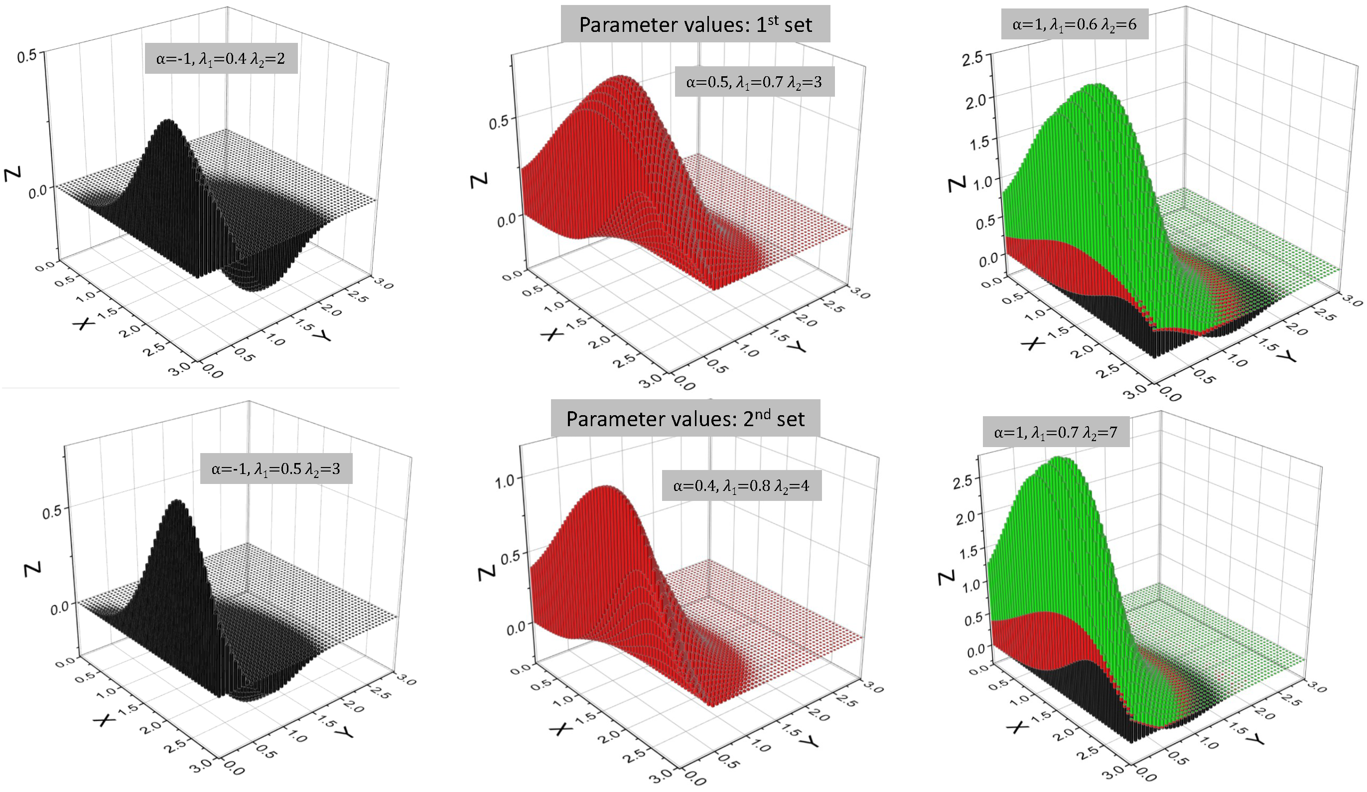
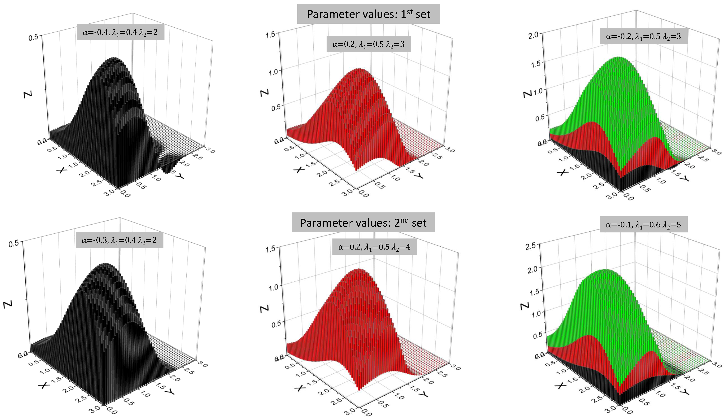
2.2. BOLiHL Distribution

This distribution is characterized by three parameters: $\alpha$, ${\lambda }_1$, and ${\lambda }_2$, where ${\lambda }_1,{\lambda }_2>0$ and $-1\le \alpha \le 1$. A pair of continuous random variables (r.vs), $(X,Y)$, is said to follow the BOLiHL distribution [14] if its cumulative distribution function (CDF) is represented below:

$$\begin{array}{cc}\hfill F_{X,Y}(x,y)& =\left(1-{\displaystyle \frac{{\lambda }_1{e}^x+{\lambda }_1+2}{2({\lambda }_1+1)}}{e}^{-{\displaystyle \frac{{\lambda }_1}{2}}(e^x-1)}\right)\times \left(1-{\displaystyle \frac{{\lambda }_2{e}^y+{\lambda }_2+2}{2({\lambda }_2+1)}}{e}^{-{\displaystyle \frac{{\lambda }_2}{2}}(e^y-1)}\right)\hfill \\ \hfill & \times \left[1+\alpha \left(1-\left(1-{\displaystyle \frac{{\lambda }_1{e}^x+{\lambda }_1+2}{2({\lambda }_1+1)}}{e}^{-{\displaystyle \frac{{\lambda }_1}{2}}(e^x-1)}\right)\right)\right.\left.\left(1-\left(1-{\displaystyle \frac{{\lambda }_2{e}^y+{\lambda }_2+2}{2({\lambda }_2+1)}}{e}^{-{\displaystyle \frac{{\lambda }_2}{2}}(e^y-1)}\right)\right)\right]\hfill \end{array}$$

(1)

for $x,y>0$, ${\lambda }_1$, ${\lambda }_2>0$, $-1\le \alpha \le 1$ and its probability density function (PDF) is defined as follows:

$$\begin{array}{cc}\hfill f_{X,Y}(x,y)& =\left({\displaystyle \frac{{\lambda }_1^2(1+e^x)}{4(1+{\lambda }_1)}}\times e^{-{\displaystyle \frac{{\lambda }_1}{2}}(e^x-1)+x}\right)\left({\displaystyle \frac{{\lambda }_2^2(1+e^y)}{4(1+{\lambda }_2)}}\times e^{-{\displaystyle \frac{{\lambda }_2}{2}}(e^y-1)+y}\right)\hfill \\ \hfill & \left[1+\alpha \left(1-2\left(1-{\displaystyle \frac{{\lambda }_1{e}^x+{\lambda }_1+2}{2({\lambda }_1+1)}}{e}^{-{\displaystyle \frac{{\lambda }_1}{2}}(e^x-1)}\right)\right)\left(1-2\left(1-{\displaystyle \frac{{\lambda }_2{e}^y+{\lambda }_2+2}{2({\lambda }_2+1)}}{e}^{-{\displaystyle \frac{{\lambda }_2}{2}}(e^y-1)}\right)\right)\right]\hfill \end{array}$$

(2)

for $x,y>0$, ${\lambda }_1$, ${\lambda }_2>0$, $-1\le \alpha \le 1$.

Figure 2 demonstrates the joint PDF of the BOLiHL model for specific parameter values, highlighting that the BOLiHL distribution displays varying shapes as the parameters are adjusted. The parameter values are (1) $\alpha =-1$, ${\lambda }_1=0.4$, ${\lambda }_2=2$; (2) $\alpha =0.5$, ${\lambda }_1=0.7$, ${\lambda }_2=3$; and (3) $\alpha =1$, ${\lambda }_1=0.6$, ${\lambda }_2=6$ and second set of parameter values are (1) $\alpha =-0.3$, ${\lambda }_1=0.4$, ${\lambda }_2=2$; (2) $\alpha =0.2$, ${\lambda }_1=0.5$, ${\lambda }_2=4$; and (3) $\alpha =-0.1$, ${\lambda }_1=0.6$, ${\lambda }_2=5$.

Survival function for the BOLiHL distribution can be expressed as:

$$\begin{array}{cc}\hfill S(x,y)& =\left({\displaystyle \frac{{\lambda }_1{e}^x+{\lambda }_1+2}{2({\lambda }_1+1)}}{e}^{-{\displaystyle \frac{{\lambda }_1}{2}}(e^x-1)}\right)\left({\displaystyle \frac{{\lambda }_2{e}^y+{\lambda }_2+2}{2({\lambda }_2+1)}}{e}^{-{\displaystyle \frac{{\lambda }_2}{2}}(e^y-1)}\right)\hfill \\ \hfill & \times \left[1+\alpha \left(1-{\displaystyle \frac{{\lambda }_1{e}^x+{\lambda }_1+2}{2({\lambda }_1+1)}}{e}^{-{\displaystyle \frac{{\lambda }_1}{2}}(e^x-1)}\right)\left(1-{\displaystyle \frac{{\lambda }_2{e}^y+{\lambda }_2+2}{2({\lambda }_2+1)}}{e}^{-{\displaystyle \frac{{\lambda }_2}{2}}(e^y-1)}\right)\right]\hfill \end{array}$$

(3)

The hazard rate function (HRF) of the BOLiHL model is

$$\begin{array}{cc}\hfill h(x,y)=& {\displaystyle \frac{\left(\frac{{\lambda }_1^2(1+e^x)}{4(1+{\lambda }_1)}\times e^{-\frac{{\lambda }_1}{2}(e^x-1)+x}\right)}{\left(\frac{{\lambda }_1{e}^x+{\lambda }_1+2}{2({\lambda }_1+1)}{e}^{-\frac{{\lambda }_1}{2}(e^x-1)}\right)}}\hfill \\ \hfill & \times {\displaystyle \frac{\left(\frac{{\lambda }_2^2(1+e^y)}{4(1+{\lambda }_2)}\times e^{-\frac{{\lambda }_2}{2}(e^y-1)+y}\right)}{\left(\frac{{\lambda }_2{e}^y+{\lambda }_2+2}{2({\lambda }_2+1)}{e}^{-\frac{{\lambda }_2}{2}(e^y-1)}\right)}}\hfill \\ \hfill & \times {\displaystyle \frac{\left[1+\alpha \left(1-2\left(1-\frac{{\lambda }_1{e}^x+{\lambda }_1+2}{2({\lambda }_1+1)}{e}^{-\frac{{\lambda }_1}{2}(e^x-1)}\right)\right)\right]\times \left(1-2\left(1-\frac{{\lambda }_2{e}^y+{\lambda }_2+2}{2({\lambda }_2+1)}{e}^{-\frac{{\lambda }_2}{2}(e^y-1)}\right)\right)}{\left[1+\alpha \left(1-\frac{{\lambda }_1{e}^x+{\lambda }_1+2}{2({\lambda }_1+1)}{e}^{-\frac{{\lambda }_1}{2}(e^x-1)}\right)\times \left(1-\frac{{\lambda }_2{e}^y+{\lambda }_2+2}{2({\lambda }_2+1)}{e}^{-\frac{{\lambda }_2}{2}(e^y-1)}\right)\right]}}\hfill \end{array}$$

(4)

Figure 3 demonstrates the joint HRF of the BOLiHL model for specific parameter values, highlighting that the BOLiHL distribution displays a decreased failure rate as the parameters are adjusted. The parameter values are (1) $\alpha =-0.4$, ${\lambda }_1=0.4$, ${\lambda }_2=2$; (2) $\alpha =0.2$, ${\lambda }_1=0.5$, ${\lambda }_2=3$; and (3) $\alpha =-0.2$, ${\lambda }_1=0.5$, ${\lambda }_2=3$ and the second set of parameter values are (1) $\alpha =-1$, ${\lambda }_1=0.5$, ${\lambda }_2=5$; (2) $\alpha =0.3$, ${\lambda }_1=0.7$, ${\lambda }_2=7$; and (3) $\alpha =-0.5$, ${\lambda }_1=0.8$, ${\lambda }_2=6$.

Now, we look at the properties of the distribution, as BOLiHL distribution possesses both positive and negative quadrant dependence. From the simulation study, we were able to observe that if the sample size increases, the value of bias and Mean Squared Error (MSE) of the estimates decreases. Also, maximum likelihood estimators (MLEs) are more accurate in estimating the true parameter values. Thus, the proposed model produces estimates that are consistent. The marginal distribution’s advantage lies in its single parameter, which governs the shape of the distribution. This shape can vary, being left-skewed, right-skewed, or nearly symmetric. Such flexibility makes the distribution a valuable tool for data scientists, enabling them to model various types of data sets effectively [15,16].

3. Maximum Likelihood Estimation

Suppose that there are n independent pairs of components $(X_{1i},Y_{2i})$, $i=1\cdots n$ under experiment, based on a PrTIICS (n, m, $R1$, …, $Rm$). The likelihood equation for PrTIICS was proposed by [11,12] and is expressed as:

$$L(\alpha ,{\lambda }_1,{\lambda }_2)=S\prod _{i=1}^m{f}_{XY}(X_{i:m:n},Y_{i:m:n},\alpha ,{\lambda }_1,{\lambda }_2){[1-F_{XY}(X_{i:m:n},Y_{i:m:n},\alpha ,{\lambda }_1,{\lambda }_2)]}^{R_i}$$

(5)

where S is the constant and does not depend on any of the parameters $\alpha ,{\lambda }_1,{\lambda }_2$.

$$S=n(n-R_1-1)\cdots \left(n-\sum _{i=1}^{m-1}(R_i+1)\right).$$

So, it can be omitted during the maximization process. $R_i$ is the censoring scheme (CS), and where $i=1,2,\cdots ,m$, m is the completely observed failure time. For more details, one can refer to [7,17]. Consider CDF and PDF given in Equations (1) and (2). Taking the logarithm on both sides, we obtain

$$\begin{array}{cc}\hfill logL(\alpha ,{\lambda }_1,{\lambda }_2)& =logC+log\left(\prod _{i=1}^m{f}_{XY}(X_{i:m:n},Y_{i:m:n},\alpha ,{\lambda }_1,{\lambda }_2){[1-F_{XY}(X_{i:m:n},Y_{i:m:n},\alpha ,{\lambda }_1,{\lambda }_2)]}^{R_i}\right)\hfill \\ \hfill & =logC+\sum _{i=1}^{m}log\left(f_{XY}(X_{i:m:n},Y_{i:m:n},\alpha ,{\lambda }_1,{\lambda }_2){[1-F_{XY}(X_{i:m:n},Y_{i:m:n},\alpha ,{\lambda }_1,{\lambda }_2)]}^{R_i}\right)\hfill \\ \hfill & =\sum _{i=1}^m\left({\displaystyle \frac{{\lambda }_1^2(1+e^{x_{i:m:n}})}{4(1+{\lambda }_1)}}{e}^{-{\displaystyle \frac{{\lambda }_1}{2}}(e^{x_{i:m:n}}-1)+x_{i:m:n}}{\displaystyle \frac{{\lambda }_2^2(1+e^{y_{i:m:n}})}{4(1+{\lambda }_2)}}{e}^{-{\displaystyle \frac{{\lambda }_2}{2}}(e^{y_{i:m:n}}-1)+y_{i:m:n}}\right)\hfill \\ \hfill & \left[1+\alpha \left(1-2\left(1-{\displaystyle \frac{{\lambda }_1{e}^{x_{i:m:n}}+{\lambda }_1+2}{2({\lambda }_1+1)}}{e}^{-{\displaystyle \frac{{\lambda }_1}{2}}(e^{x_{i:m:n}}-1)}\right)\right)\right.\hfill \\ \hfill & \left.\left(1-2\left(1-{\displaystyle \frac{{\lambda }_2{e}^{y_{i:m:n}}+{\lambda }_2+2}{2({\lambda }_2+1)}}{e}^{-{\displaystyle \frac{{\lambda }_2}{2}}(e^{y_{i:m:n}}-1)}\right)\right)\right]\hfill \\ \hfill & +\sum _{i=1}^m{R}_{i}log\left(1-\left(\left(1-{\displaystyle \frac{{\lambda }_1{e}^{x_{i:m:n}}+{\lambda }_1+2}{2({\lambda }_1+1)}}{e}^{-{\displaystyle \frac{{\lambda }_1}{2}}(e^{x_{i:m:n}}-1)}\right)\right.\right.\hfill \\ \hfill & \left(1-{\displaystyle \frac{{\lambda }_2{e}^{y_{i:m:n}}+{\lambda }_2+2}{2({\lambda }_2+1)}}{e}^{-{\displaystyle \frac{{\lambda }_2}{2}}(e^{y_{i:m:n}}-1)}\right)\hfill \\ \hfill & \left[1+\alpha \left(1-\left(1-{\displaystyle \frac{{\lambda }_1{e}^{x_{i:m:n}}+{\lambda }_1+2}{2({\lambda }_1+1)}}{e}^{-{\displaystyle \frac{{\lambda }_1}{2}}(e^{x_{i:m:n}}-1)}\right)\right)\right.\hfill \\ \hfill & \left.\left.\left.\left(1-\left(1-{\displaystyle \frac{{\lambda }_2{e}^{y_{i:m:n}}+{\lambda }_2+2}{2({\lambda }_2+1)}}{e}^{-{\displaystyle \frac{{\lambda }_2}{2}}(e^{y_{i:m:n}}-1)}\right)\right)\right]\right)\right)\hfill \\ \hfill & =2mlog{\lambda }_1-mlog\left(4{\lambda }_1+4\right)+\sum _{i=1}^{m}log\left(e^{x_{i:m:n}}+1\right)\hfill \\ \hfill & -{\displaystyle \frac{1}{2}}{\lambda }_1\sum _{i=1}^m\left(e^{x_{i:m:n}}-1\right)+\sum _{i=1}^m{x}_i+2mlog{\lambda }_2-mlog\left(4{\lambda }_2+4\right)\hfill \\ \hfill & +\sum _{i=1}^{m}log\left(e^{y_{i:m:n}}+1\right)-{\displaystyle \frac{1}{2}}{\lambda }_2\sum _{i=1}^m\left(e^{y_{i:m:n}}-1\right)+\sum _{i=1}^m{y}_i\hfill \\ \hfill & +\sum _{i=1}^{m}log\left(1+\alpha \left(1-2\left(1-{\displaystyle \frac{e^{-\frac{1}{2}{\lambda }_1\left(e^{x_{i:m:n}}-1\right)}\left({\lambda }_1+{\lambda }_1{e}^{x_{i:m:n}}+2\right)}{2\left({\lambda }_1+1\right)}}\right)\right)\right.\hfill \\ \hfill & \left.\times \left(1-2\left(1-{\displaystyle \frac{e^{-\frac{1}{2}{\lambda }_2\left(e^{y_{i:m:n}}-1\right)}\left({\lambda }_2+{\lambda }_2{e}^{y_{i:m:n}}+2\right)}{2\left({\lambda }_2+1\right)}}\right)\right)\right)\hfill \\ \hfill & +\sum _{i=1}^m{R}_{i}log\left(1-\left(\left(1-{\displaystyle \frac{{\lambda }_1{e}^{x_{i:m:n}}+{\lambda }_1+2}{2({\lambda }_1+1)}}{e}^{-{\displaystyle \frac{{\lambda }_1}{2}}(e^{x_{i:m:n}}-1)}\right)\right.\right.\hfill \\ \hfill & \left(1-{\displaystyle \frac{{\lambda }_2{e}^{y_{i:m:n}}+{\lambda }_2+2}{2({\lambda }_2+1)}}{e}^{-{\displaystyle \frac{{\lambda }_2}{2}}(e^{y_{i:m:n}}-1)}\right)\hfill \\ \hfill & \left[1+\alpha \left(1-\left(1-{\displaystyle \frac{{\lambda }_1{e}^{x_{i:m:n}}+{\lambda }_1+2}{2({\lambda }_1+1)}}{e}^{-{\displaystyle \frac{{\lambda }_1}{2}}(e^{x_{i:m:n}}-1)}\right)\right)\right.\hfill \\ \hfill & \left.\left.\left.\left(1-\left(1-{\displaystyle \frac{{\lambda }_2{e}^{y_{i:m:n}}+{\lambda }_2+2}{2({\lambda }_2+1)}}{e}^{-{\displaystyle \frac{{\lambda }_2}{2}}(e^{y_{i:m:n}}-1)}\right)\right)\right]\right)\right)\hfill \end{array}$$

(6)

The first derivatives of Equation (6) with respect to the unknown parameters $\alpha ,{\lambda }_1$ and ${\lambda }_2$ are derived as follows:

$$\begin{array}{cc}\hfill {\displaystyle \frac{\partial logL}{\partial {\lambda }_1}}& ={\displaystyle \frac{2m_1}{{\lambda }_1}}-{\displaystyle \frac{4m_1}{4{\lambda }_1+4}}-{\displaystyle \frac{1}{2}}\sum _{i=1}^n(e^{x_{i:m:n}}-1)\hfill \\ \hfill & +\sum _{i=1}^n\left(-{\displaystyle \frac{2\alpha ·\left(1-2\left({\eta }_1(y_{i:m:n};{\lambda }_2)\right)\left(\delta (x_{i:m:n};{\lambda }_1)\right)\right)}{1+\alpha ·\left(1-2\left({\eta }_1(y_{i:m:n};{\lambda }_2)\right)\right)\left(1-2\left({\eta }_2(x_{i:m:n};{\lambda }_1)\right)\right)}}\right)+\sum _{i=1}^m{R}_i\hfill \\ \hfill & {\displaystyle \frac{\begin{array}{c}-({\eta }_1(y_{i:m:n};{\lambda }_2){\eta }_2(x_{i:m:n};{\lambda }_1)K_1(x_{i:m:n},y_{i:m:n};{\lambda }_1,{\lambda }_2)-K_2(x_{i:m:n},y_{i:m:n};{\lambda }_2,{\lambda }_1)\hfill \\ -K_3(y_{i:m:n},x_{i:m:n};{\lambda }_2,{\lambda }_1)-{\eta }_1(y_{i:m:n};{\lambda }_2)\left(\delta (x_{i:m:n};{\lambda }_1)\right)\psi (x_{i:m:n},y_{i:m:n};{\lambda }_1,{\lambda }_2))\hfill \end{array}}{1-{\eta }_1(y_{i:m:n};{\lambda }_2){\eta }_2(x_{i:m:n};{\lambda }_1)\psi (x_{i:m:n},y_{i:m:n};{\lambda }_1,{\lambda }_2)}}\hfill \end{array}$$

(7)

$$\begin{array}{cc}\hfill {\displaystyle \frac{\partial logL}{\partial {\lambda }_2}}& ={\displaystyle \frac{2m_2}{{\lambda }_2}}-{\displaystyle \frac{4m_2}{4{\lambda }_2+4}}-{\displaystyle \frac{1}{2}}\sum _{i=1}^n(e^{y_{i:m:n}}-1)\hfill \\ \hfill & +\sum _{i=1}^n-{\displaystyle \frac{2\alpha ·\left(1-2\left({\eta }_2(x_{i:m:n};{\lambda }_1)\left({\delta }_1(y_{i:m:n};{\lambda }_2)\right)\right)\right)}{1+\alpha ·\left(1-2\left({\eta }_2(x_{i:m:n};{\lambda }_1)\right)\right)\left(1-2\left({\eta }_1(y_{i:m:n};{\lambda }_2)\right)\right)}}+\sum _{i=1}^m{R}_i\hfill \\ \hfill & {\displaystyle \frac{\begin{array}{c}\hfill -({\eta }_2(x_{i:m:n};{\lambda }_1){\eta }_1(y_{i:m:n};{\lambda }_2)K_4(x_{i:m:n},y_{i:m:n};{\lambda }_1,{\lambda }_2)-K_5(y_{i:m:n},x_{i:m:n};{\lambda }_1,{\lambda }_2)\\ -K_6(y_{i:m:n},x_{i:m:n};{\lambda }_1,{\lambda }_2)-{\eta }_2(x_{i:m:n};{\lambda }_1)\left({\delta }_1(y_{i:m:n};{\lambda }_2)\right){\psi }_1(x_{i:m:n},y_{i:m:n};{\lambda }_2,{\lambda }_1))\hfill \end{array}}{1-{\eta }_2(x_{i:m:n};{\lambda }_1){\eta }_1(y_{i:m:n};{\lambda }_2){\psi }_1(x_{i:m:n},y_{i:m:n};{\lambda }_2,{\lambda }_1)}}\hfill \end{array}$$

(8)

$$\begin{array}{cc}\hfill {\displaystyle \frac{\partial logL}{\partial \alpha }}& =\sum _{i=1}^n{\displaystyle \frac{\left(1-2{\eta }_2(x_{i:m:n};{\lambda }_1)\right)\left(1-2{\eta }_1(y_{i:m:n};{\lambda }_2)\right)}{1+\alpha ·\left(1-2{\eta }_2(x_{i:m:n};{\lambda }_1)\right)\left(1-2{\eta }_1(y_{i:m:n};{\lambda }_2)\right)}}+\sum _{i=1}^m{R}_i\hfill \\ \hfill & -{\displaystyle \frac{\begin{array}{cc}\hfill & \left({\lambda }_1{\mathrm{e}}^{x_{i:m:n}}+{\lambda }_1+2\right){\eta }_2(x_{i:m:n};{\lambda }_1)\left({\lambda }_2{\mathrm{e}}^{y_{i:m:n}}+{\lambda }_2+2\right)\hfill \\ \hfill & ·{\mathrm{e}}^{-\frac{{\lambda }_2\left({\mathrm{e}}^{y_{i:m:n}}-1\right)}{2}-\frac{{\lambda }_1\left({\mathrm{e}}^{x_{i:m:n}}-1\right)}{2}}{\eta }_1(y_{i:m:n};{\lambda }_2)\hfill \end{array}}{4\left({\lambda }_1+1\right)\left({\lambda }_2+1\right)\left(1-{\eta }_2(x_{i:m:n};{\lambda }_1){\eta }_1(y_{i:m:n};{\lambda }_2){\psi }_1(x_{i:m:n},y_{i:m:n};{\lambda }_2,{\lambda }_1)\right)}}\hfill \end{array}$$

(9)

where

$${\eta }_1(y_{i:m:n};{\lambda }_2)=\left(1-{\displaystyle \frac{\left({\lambda }_2{\mathrm{e}}^{y_{i:m:n}}+{\lambda }_2+2\right){\mathrm{e}}^{-\frac{{\lambda }_2\left({\mathrm{e}}^{y_{i:m:n}}-1\right)}{2}}}{2\left({\lambda }_2+1\right)}}\right)$$

$${\eta }_2(x_{i:m:n};{\lambda }_1)=\left(1-{\displaystyle \frac{\left({\mathrm{e}}^{x_{i:m:n}}{\lambda }_1+{\lambda }_1+2\right){\mathrm{e}}^{-\frac{\left({\mathrm{e}}^{x_{i:m:n}}-1\right){\lambda }_1}{2}}}{2\left({\lambda }_1+1\right)}}\right)$$

$$K_1(x_{i:m:n},y_{i:m:n};{\lambda }_1,{\lambda }_2)={\displaystyle \frac{\alpha \left({\mathrm{e}}^{x_{i:m:n}}+1\right)\left({\lambda }_2{\mathrm{e}}^{y_{i:m:n}}+{\lambda }_2+2\right){\mathrm{e}}^{-\frac{\left({\mathrm{e}}^{x_{i:m:n}}-1\right){\lambda }_1}{2}-\frac{{\lambda }_2\left({\mathrm{e}}^{y_{i:m:n}}-1\right)}{2}}}{4\left({\lambda }_2+1\right)\left({\lambda }_1+1\right)}}$$

$$\begin{array}{c}\hfill K_2(x_{i:m:n},y_{i:m:n};{\lambda }_2,{\lambda }_1)={\displaystyle \frac{\alpha \left({\mathrm{e}}^{x_{i:m:n}}-1\right)\left({\lambda }_2{\mathrm{e}}^{y_{i:m:n}}+{\lambda }_2+2\right)\left({\mathrm{e}}^{x_{i:m:n}}{\lambda }_1+{\lambda }_1+2\right){\mathrm{e}}^{-\frac{\left({\mathrm{e}}^{x_{i:m:n}}-1\right){\lambda }_1}{2}-\frac{{\lambda }_2\left({\mathrm{e}}^{y_{i:m:n}}-1\right)}{2}}}{8\left({\lambda }_2+1\right)\left({\lambda }_1+1\right)}}\end{array}$$

$$K_3(y_{i:m:n},x_{i:m:n};{\lambda }_2,{\lambda }_1)={\displaystyle \frac{\alpha \left({\lambda }_2{\mathrm{e}}^{y_{i:m:n}}+{\lambda }_2+2\right)\left({\mathrm{e}}^{x_{i:m:n}}{\lambda }_1+{\lambda }_1+2\right){\mathrm{e}}^{-\frac{\left({\mathrm{e}}^{x_{i:m:n}}-1\right){\lambda }_1}{2}-\frac{{\lambda }_2\left({\mathrm{e}}^{y_{i:m:n}}-1\right)}{2}}}{4\left({\lambda }_2+1\right){\left({\lambda }_1+1\right)}^2}}$$

$$\begin{array}{cc}\hfill \delta (x_{i:m:n};{\lambda }_1)=& \left(-{\displaystyle \frac{\left({\mathrm{e}}^{x_{i:m:n}}+1\right){\mathrm{e}}^{-\frac{\left({\mathrm{e}}^{x_{i:m:n}}-1\right){\lambda }_1}{2}}}{2\left({\lambda }_1+1\right)}}\right.+{\displaystyle \frac{\left({\mathrm{e}}^{x_{i:m:n}}-1\right)\left({\mathrm{e}}^{x_{i:m:n}}{\lambda }_1+{\lambda }_1+2\right){\mathrm{e}}^{-\frac{\left({\mathrm{e}}^{x_{i:m:n}}-1\right){\lambda }_1}{2}}}{4\left({\lambda }_1+1\right)}}\hfill \\ \hfill & \left.+{\displaystyle \frac{\left({\mathrm{e}}^{x_{i:m:n}}{\lambda }_1+{\lambda }_1+2\right){\mathrm{e}}^{-\frac{\left({\mathrm{e}}^{x_{i:m:n}}-1\right){\lambda }_1}{2}}}{2{\left({\lambda }_1+1\right)}^2}}\right)\hfill \end{array}$$

$$\psi (x_{i:m:n},y_{i:m:n};{\lambda }_1,{\lambda }_2)=\left({\displaystyle \frac{\alpha \left({\lambda }_2{\mathrm{e}}^{y_{i:m:n}}+{\lambda }_2+2\right)\left({\mathrm{e}}^{x_{i:m:n}}{\lambda }_1+{\lambda }_1+2\right){\mathrm{e}}^{-\frac{\left({\mathrm{e}}^{x_{i:m:n}}-1\right){\lambda }_1}{2}-\frac{{\lambda }_2\left({\mathrm{e}}^{y_{i:m:n}}-1\right)}{2}}}{4\left({\lambda }_2+1\right)\left({\lambda }_1+1\right)}}+1\right)$$

$$K_4(x_{i:m:n},y_{i:m:n};{\lambda }_1,{\lambda }_2)={\displaystyle \frac{\alpha \left({\mathrm{e}}^{y_{i:m:n}}+1\right)\left({\lambda }_1{\mathrm{e}}^{x_{i:m:n}}+{\lambda }_1+2\right){\mathrm{e}}^{-\frac{\left({\mathrm{e}}^{y_{i:m:n}}-1\right){\lambda }_2}{2}-\frac{{\lambda }_1\left({\mathrm{e}}^{x_{i:m:n}}-1\right)}{2}}}{4\left({\lambda }_1+1\right)\left({\lambda }_2+1\right)}}$$

$$\begin{array}{c}\hfill K_5(y_{i:m:n},x_{i:m:n};{\lambda }_1,{\lambda }_2)={\displaystyle \frac{\alpha \left({\mathrm{e}}^{y_{i:m:n}}-1\right)\left({\lambda }_1{\mathrm{e}}^{x_{i:m:n}}+{\lambda }_1+2\right)\left({\mathrm{e}}^{y_{i:m:n}}{\lambda }_2+{\lambda }_2+2\right){\mathrm{e}}^{-\frac{\left({\mathrm{e}}^{y_{i:m:n}}-1\right){\lambda }_2}{2}-\frac{{\lambda }_1\left({\mathrm{e}}^{x_{i:m:n}}-1\right)}{2}}}{8\left({\lambda }_1+1\right)\left({\lambda }_2+1\right)}}\end{array}$$

$$K_6(y_{i:m:n},x_{i:m:n};{\lambda }_1,{\lambda }_2)={\displaystyle \frac{\alpha \left({\lambda }_1{\mathrm{e}}^{x_{i:m:n}}+{\lambda }_1+2\right)\left({\mathrm{e}}^{y_{i:m:n}}{\lambda }_2+{\lambda }_2+2\right){\mathrm{e}}^{-\frac{\left({\mathrm{e}}^{y_{i:m:n}}-1\right){\lambda }_2}{2}-\frac{{\lambda }_1\left({\mathrm{e}}^{x_{i:m:n}}-1\right)}{2}}}{4\left({\lambda }_1+1\right){\left({\lambda }_2+1\right)}^2}}$$

$$\begin{array}{cc}\hfill {\delta }_1(y_{i:m:n};{\lambda }_2)=& \left(-{\displaystyle \frac{\left({\mathrm{e}}^{y_{i:m:n}}+1\right){\mathrm{e}}^{-\frac{\left({\mathrm{e}}^{y_{i:m:n}}-1\right){\lambda }_2}{2}}}{2\left({\lambda }_2+1\right)}}\right.+{\displaystyle \frac{\left({\mathrm{e}}^{y_{i:m:n}}-1\right)\left({\mathrm{e}}^{y_{i:m:n}}{\lambda }_2+{\lambda }_2+2\right){\mathrm{e}}^{-\frac{\left({\mathrm{e}}^{y_{i:m:n}}-1\right){\lambda }_2}{2}}}{4\left({\lambda }_2+1\right)}}\hfill \\ \hfill & \left.+{\displaystyle \frac{\left({\mathrm{e}}^{y_{i:m:n}}{\lambda }_2+{\lambda }_2+2\right){\mathrm{e}}^{-\frac{\left({\mathrm{e}}^{y_{i:m:n}}-1\right){\lambda }_2}{2}}}{2{\left({\lambda }_2+1\right)}^2}}\right)\hfill \end{array}$$

$${\psi }_1(x_{i:m:n},y_{i:m:n};{\lambda }_2,{\lambda }_1)=\left({\displaystyle \frac{\alpha \left({\lambda }_1{\mathrm{e}}^{x_{i:m:n}}+{\lambda }_1+2\right)\left({\mathrm{e}}^{y_{i:m:n}}{\lambda }_2+{\lambda }_2+2\right){\mathrm{e}}^{-\frac{\left({\mathrm{e}}^{y_{i:m:n}}-1\right){\lambda }_2}{2}-\frac{{\lambda }_1\left({\mathrm{e}}^{x_{i:m:n}}-1\right)}{2}}}{4\left({\lambda }_1+1\right)\left({\lambda }_2+1\right)}}+1\right)$$

$${\eta }_2(x_{i:m:n};{\lambda }_1)=\left(1-{\displaystyle \frac{\left({\mathrm{e}}^{x_{i:m:n}}{\lambda }_1+{\lambda }_1+2\right){\mathrm{e}}^{-\frac{\left({\mathrm{e}}^{x_{i:m:n}}-1\right){\lambda }_1}{2}}}{2\left({\lambda }_1+1\right)}}\right)$$

$${\eta }_1(y_{i:m:n};{\lambda }_2)=\left(1-{\displaystyle \frac{\left({\lambda }_2{\mathrm{e}}^{y_{i:m:n}}+{\lambda }_2+2\right){\mathrm{e}}^{-\frac{{\lambda }_2\left({\mathrm{e}}^{y_{i:m:n}}-1\right)}{2}}}{2\left({\lambda }_2+1\right)}}\right)$$

$${\psi }_1(x_{i:m:n},y_{i:m:n};{\lambda }_2,{\lambda }_1)=\left({\displaystyle \frac{\alpha \left({\lambda }_1{\mathrm{e}}^{x_{i:m:n}}+{\lambda }_1+2\right)\left({\mathrm{e}}^{y_{i:m:n}}{\lambda }_2+{\lambda }_2+2\right){\mathrm{e}}^{-\frac{\left({\mathrm{e}}^{y_{i:m:n}}-1\right){\lambda }_2}{2}-\frac{{\lambda }_1\left({\mathrm{e}}^{x_{i:m:n}}-1\right)}{2}}}{4\left({\lambda }_1+1\right)\left({\lambda }_2+1\right)}}+1\right)$$

The MLEs of $\alpha$, ${\lambda }_1$, and ${\lambda }_2$ for the BOLiHL distribution parameters under the PrTIICS are obtained by solving the above non-linear equations, setting them equal to zero. These equations are highly difficult to solve directly; therefore, a nonlinear optimization algorithm, such as the Newton–Raphson method, is used. The Newton–Raphson method is applied to determine the root of a system of non-linear equations [18]. In numerical analysis, Newton’s method is an iterative approach used to find increasingly accurate approximations to the roots (or zeroes) of a real-valued function [19]. Any zero-finding method, such as Newton–Raphson, can also finding a function’s minimum or maximum by identifying a zero in its first derivative. In the MLE, this method is introduced to estimate the unknown parameters in optimisation algorithm.

The asymptotic confidence interval (ACI) for the parameters of the BOLiHl distribution under PrTIICS can be estimated through numerical inversion of the Fisher information matrix. The Fisher information matrix $I\left(\mathrm{\Theta }\right)$ which relates to the asymptotic variance–covariance matrix of the MLE of the parameters, is consists of the negative second-order derivatives of the natural logarithm of the probability function examined at $\widehat{\mathrm{\Theta }}=\left(\widehat{\alpha },{\widehat{\lambda }}_1,{\widehat{\lambda }}_2\right)$. Assume that the asymptotic variance–covariance matrix of the parameter vector $\mathrm{\Theta }$ is

$$I\left(\widehat{\mathrm{\Theta }}\right)=-E\left(\begin{array}{ccc}{I}_{\widehat{\alpha }\widehat{\alpha }}& I_{\widehat{\alpha }{\widehat{\lambda }}_1}& I_{\widehat{\alpha }{\widehat{\lambda }}_2}\\ I_{{\widehat{\lambda }}_1\widehat{\alpha }}& I_{{\widehat{\lambda }}_1{\widehat{\lambda }}_1}& I_{{\widehat{\lambda }}_1{\widehat{\lambda }}_2}\\ I_{{\widehat{\lambda }}_2\widehat{\alpha }}& I_{{\widehat{\lambda }}_2{\widehat{\lambda }}_1}& I_{{\widehat{\lambda }}_2{\widehat{\lambda }}_2}\end{array}\right)$$

(10)

where

$$V\left(\widehat{\mathrm{\Theta }}\right)=I^{-1}\left(\widehat{\mathrm{\Theta }}\right)$$

Thus, the $100(1-\gamma )\%$ confidence intervals (CIs) for the parameter $\mathrm{\Theta }$ can be derived using the asymptotic normality of the MLE as follows:

$$\widehat{\alpha }\pm z_{\gamma /2}\sqrt{I_{\widehat{\alpha }\widehat{\alpha }}},{\widehat{\lambda }}_1\pm z_{\gamma /2}\sqrt{I_{{\widehat{\lambda }}_1{\widehat{\lambda }}_1}},{\widehat{\lambda }}_2\pm z_{\gamma /2}\sqrt{I_{{\widehat{\lambda }}_2{\widehat{\lambda }}_2}}.$$

(11)

The $z_{\gamma /2}$ represents the percentile of the standard normal distribution corresponding to the cumulative probability $1-\gamma /2$. The second-order partial derivatives to construct the Fisher information matrix are:

$$\begin{array}{c}\hfill I_{\widehat{\alpha }\widehat{\alpha }}={\displaystyle \frac{{\partial }^{2}logL(\alpha ,{\lambda }_1,{\lambda }_2)}{\partial {\alpha }^2}},I_{\widehat{\alpha }{\widehat{\lambda }}_1}={\displaystyle \frac{{\partial }^{2}logL(\alpha ,{\lambda }_1,{\lambda }_2)}{\partial \alpha \partial {\lambda }_1}},I_{\widehat{\alpha }{\widehat{\lambda }}_2}={\displaystyle \frac{{\partial }^{2}logL(\alpha ,{\lambda }_1,{\lambda }_2)}{\partial \alpha \partial {\lambda }_2}}\\ \hfill I_{{\widehat{\lambda }}_1\widehat{\alpha }}={\displaystyle \frac{{\partial }^{2}logL(\alpha ,{\lambda }_1,{\lambda }_2)}{\partial {\lambda }_1\partial \alpha }},I_{{\widehat{\lambda }}_1{\widehat{\lambda }}_1}={\displaystyle \frac{{\partial }^{2}logL(\alpha ,{\lambda }_1,{\lambda }_2)}{\partial {\lambda }_1^2}},I_{{\widehat{\lambda }}_1{\widehat{\lambda }}_2}={\displaystyle \frac{{\partial }^{2}logL(\alpha ,{\lambda }_1,{\lambda }_2)}{\partial {\lambda }_1\partial {\lambda }_2}}\\ \hfill I_{{\widehat{\lambda }}_2\widehat{\alpha }}={\displaystyle \frac{{\partial }^{2}logL(\alpha ,{\lambda }_1,{\lambda }_2)}{\partial {\lambda }_2\partial \alpha }},I_{{\widehat{\lambda }}_2{\widehat{\lambda }}_1}={\displaystyle \frac{{\partial }^{2}logL(\alpha ,{\lambda }_1,{\lambda }_2)}{\partial {\lambda }_2\partial {\lambda }_1}},I_{{\widehat{\lambda }}_2{\widehat{\lambda }}_2}={\displaystyle \frac{{\partial }^{2}logL(\alpha ,{\lambda }_1,{\lambda }_2)}{\partial {\lambda }_2^2}}\end{array}$$

4. Bayesian Estimation

In this section, we explore the Bayesian estimation of the unknown parameter for the BOLiHL model under PrTIICS. In the vector of the parameters $({\lambda }_1,{\lambda }_2)$ we have used the informative prior as independent gamma prior distributions. In the copula parameter, we used non-informative prior distribution such as uniform $(a,b)$; $-1<\alpha <1$. Assume that ${\lambda }_1\sim Gamma(b_1,l_1)$ and ${\lambda }_2\sim Gamma(b_2,l_2)$ and $\alpha \sim {\displaystyle \frac{1}{l_3-b_3}}$. Gamma priors are chosen for their flexibility and conjugacy, making posterior computations more effective, specifically for scale parameters. Uniform priors, on the other hand, are non-informative and ensure minimal bias when there is restricted prior knowledge. This combination balances prior information and objectivity in the analysis. In the case of BOLiHL distribution, the independent joint prior density function of $\mathrm{\Theta }$ can be written as follows:

$$\pi \left(\mathrm{\Theta }\right)={\lambda }_1^{b_2-1}{\lambda }_2^{b_3-1}{\displaystyle \frac{1}{l_3-b_3}}{e}^{-l_3{\lambda }_2-l_2{\lambda }_1}$$

(12)

The hyperparameters of the independent joint prior can be written using the estimated mean and variance–covariance matrix obtained from the MLE technique. By equating the mean and variance of gamma priors [20], the hyperparameters can be determined as follows:

$$p_j={\displaystyle \frac{{\left[\frac{1}{L}{\sum }_{i=1}^L{\widehat{\mathrm{\Theta }}}_j^i\right]}^2}{\frac{1}{L-1}{\sum }_{i=1}^L{\left[{\widehat{\mathrm{\Theta }}}_j^i-\frac{1}{L}{\sum }_{i=1}^L{\widehat{\mathrm{\Theta }}}_j^i\right]}^2}},j=1,\dots ,p-1,$$

$$q_j={\displaystyle \frac{\frac{1}{L}{\sum }_{i=1}^L{\widehat{\mathrm{\Theta }}}_j^i}{\frac{1}{L-1}{\sum }_{i=1}^L{\left[{\widehat{\mathrm{\Theta }}}_j^i-\frac{1}{L}{\sum }_{i=1}^L{\widehat{\mathrm{\Theta }}}_j^i\right]}^2}},j=1,\dots ,p-1,$$

where L is the number of iterations. The estimated hyperparameter formula for the copula parameter can be calculated as follows:

$$p_3={\displaystyle \frac{{\left[\frac{3}{L-1}{\sum }_{i=1}^L{\widehat{\alpha }}^i-\frac{1}{L}{\sum }_{i=1}^L{\widehat{\alpha }}^i\right]}^2}{\frac{1}{L}{\sum }_{i=1}^L{\widehat{\alpha }}^i}},$$

$$q_3={\displaystyle \frac{\frac{1}{L}{\sum }_{i=1}^L{\widehat{\alpha }}^i}{\sqrt{\frac{3}{L-1}{\sum }_{i=1}^L{\left[{\widehat{\alpha }}^i-\frac{1}{L}{\sum }_{i=1}^L{\widehat{\alpha }}^i\right]}^2}}}.$$

The posterior likelihood can be calculated proportionally to the product of the likelihood function of BOLiHL distribution and the joint prior density. The joint posterior density of $\mathrm{\Theta }$ is

$$\mathrm{\Pi }\left(\mathrm{\Theta }\right|x_{i:m:n},y_{i:m:n})\propto L(x_{i:m:n},y_{i:m:n},\mathrm{\Theta })\times \pi \left(\mathrm{\Theta }\right)$$

Then, the joint posterior density $\mathrm{\Theta }$ is

$$\begin{array}{cc}\hfill \mathrm{\Pi }\left(\mathrm{\Theta }\right|x_{i:m:n},y_{i:m:n})\propto \prod _{i=1}^m& \left(\left(\left({\displaystyle \frac{{\lambda }_1^2(1+e^{x_{i:m:n}})}{4(1+{\lambda }_1)}}\times e^{-{\displaystyle \frac{{\lambda }_1}{2}}(e^{x_{i:m:n}}-1)+x_{i:m:n}}\right)\right.\right.\hfill \\ \hfill & \left.\left({\displaystyle \frac{{\lambda }_2^2(1+e^{y_{i:m:n}})}{4(1+{\lambda }_2)}}\times e^{-{\displaystyle \frac{{\lambda }_2}{2}}(e^{y_{i:m:n}}-1)+y_{i:m:n}}\right)\right)\hfill \\ \hfill & \times \left(1+\alpha \left(1-2\left(1-{\displaystyle \frac{{\lambda }_1{e}^{x_{i:m:n}}+{\lambda }_1+2}{2({\lambda }_1+1)}}{e}^{-{\displaystyle \frac{{\lambda }_1}{2}}(e^{x_{i:m:n}}-1)}\right)\right)\right.\hfill \\ \hfill & \times \left.\left(1-2\left(1-{\displaystyle \frac{{\lambda }_2{e}^{y_{i:m:n}}+{\lambda }_2+2}{2({\lambda }_2+1)}}{e}^{-{\displaystyle \frac{{\lambda }_2}{2}}(e^{y_{i:m:n}}-1)}\right)\right)\right)\hfill \\ \hfill & \left(1-\left(\left(1-{\displaystyle \frac{{\lambda }_1{e}^{x_{i:m:n}}+{\lambda }_1+2}{2({\lambda }_1+1)}}{e}^{-{\displaystyle \frac{{\lambda }_1}{2}}(e^{x_{i:m:n}}-1)}\right)\right.\right.\hfill \\ \hfill & \times \left(1-{\displaystyle \frac{{\lambda }_2{e}^{y_{i:m:n}}+{\lambda }_2+2}{2({\lambda }_2+1)}}{e}^{-{\displaystyle \frac{{\lambda }_2}{2}}(e^{y_{i:m:n}}-1)}\right)\hfill \\ \hfill & \times \left[1+\alpha \left(1-\left(1-{\displaystyle \frac{{\lambda }_1{e}^{x_{i:m:n}}+{\lambda }_1+2}{2({\lambda }_1+1)}}{e}^{-{\displaystyle \frac{{\lambda }_1}{2}}(e^{x_{i:m:n}}-1)}\right)\right)\right.\hfill \\ \hfill & \left.{\left.\left.\left.\left(1-\left(1-{\displaystyle \frac{{\lambda }_2{e}^{y_{i:m:n}}+{\lambda }_2+2}{2({\lambda }_2+1)}}{e}^{-{\displaystyle \frac{{\lambda }_2}{2}}(e^{y_{i:m:n}}-1)}\right)\right)\right]\right)\right)}^{R_i}\right)\times {\lambda }_1^{b_1-1}{\lambda }_2^{b_2-1}{\displaystyle \frac{1}{l_3-b_3}}\hfill \\ \hfill & e^{-l_1{\lambda }_1-l_2{\lambda }_2}\hfill \end{array}$$

(13)

For the BOLiHL distribution based on PrTIICS, the full conditional posterior distributions of the parameters are presented below:

$$\begin{array}{cc}\hfill \mathrm{\Pi }\left({\lambda }_1\right|{\lambda }_2,x_{i:m:n},y_{i:m:n})& ={\lambda }_1^{b_1-1}{e}^{-l_1{\lambda }_1}\prod _{i=1}^m[\left({\displaystyle \frac{{\lambda }_1^2(1+e^{x_{i:m:n}})}{4(1+{\lambda }_1)}}{e}^{-{\displaystyle \frac{{\lambda }_1}{2}}(e^{x_{i:m:n}}-1)+x_{i:m:n}}\right)\hfill \\ \hfill & \times \left(1+\alpha \left(1-2\left(1-{\displaystyle \frac{{\lambda }_1{e}^{x_{i:m:n}}+{\lambda }_1+2}{2({\lambda }_1+1)}}{e}^{-{\displaystyle \frac{{\lambda }_1}{2}}(e^{x_{i:m:n}}-1)}\right)\right)\right)\hfill \\ \hfill & \times \left(1-2\left(1-{\displaystyle \frac{{\lambda }_2{e}^{y_{i:m:n}}+{\lambda }_2+2}{2({\lambda }_2+1)}}{e}^{-{\displaystyle \frac{{\lambda }_2}{2}}(e^{y_{i:m:n}}-1)}\right)\right)]\hfill \\ \hfill & \prod _{i=1}^m\left[\left(1-\left(\left(1-{\displaystyle \frac{{\lambda }_1{e}^{x_{i:m:n}}+{\lambda }_1+2}{2({\lambda }_1+1)}}{e}^{-{\displaystyle \frac{{\lambda }_1}{2}}(e^{x_{i:m:n}}-1)}\right)\right.\right.\right.\hfill \\ \hfill & \times \left[1+\alpha \left(1-\left(1-{\displaystyle \frac{{\lambda }_1{e}^{x_{i:m:n}}+{\lambda }_1+2}{2({\lambda }_1+1)}}{e}^{-{\displaystyle \frac{{\lambda }_1}{2}}(e^{x_{i:m:n}}-1)}\right)\right)\right.\hfill \\ \hfill & \left.{\left.\left.\left.\left(1-\left(1-{\displaystyle \frac{{\lambda }_2{e}^{y_{i:m:n}}+{\lambda }_2+2}{2({\lambda }_2+1)}}{e}^{-{\displaystyle \frac{{\lambda }_2}{2}}(e^{y_{i:m:n}}-1)}\right)\right)\right]\right)\right)}^{R_i}\right]\hfill \end{array}$$

(14)

$$\begin{array}{cc}\hfill \mathrm{\Pi }\left({\lambda }_2\right|{\lambda }_1,x_{i:m:n},y_{i:m:n})& ={\lambda }_2^{b_2-1}{e}^{-l_2{\lambda }_2}\prod _{i=1}^m[\left({\displaystyle \frac{{\lambda }_2^2(1+e^{y_{i:m:n}})}{4(1+{\lambda }_2)}}{e}^{-{\displaystyle \frac{{\lambda }_2}{2}}(e^{y_{i:m:n}}-1)+y_{i:m:n}}\right)\hfill \\ \hfill & \times \left(1+\alpha \left(1-2\left(1-{\displaystyle \frac{{\lambda }_1{e}^{x_{i:m:n}}+{\lambda }_1+2}{2({\lambda }_1+1)}}{e}^{-{\displaystyle \frac{{\lambda }_1}{2}}(e^{x_{i:m:n}}-1)}\right)\right)\right)\hfill \\ \hfill & \times \left(1-2\left(1-{\displaystyle \frac{{\lambda }_2{e}^{y_{i:m:n}}+{\lambda }_2+2}{2({\lambda }_2+1)}}{e}^{-{\displaystyle \frac{{\lambda }_2}{2}}(e^{y_{i:m:n}}-1)}\right)\right)]\hfill \\ \hfill & \prod _{i=1}^m\left[\left(1-\left(\left(1-{\displaystyle \frac{{\lambda }_2{e}^{y_{i:m:n}}+{\lambda }_2+2}{2({\lambda }_2+1)}}{e}^{-{\displaystyle \frac{{\lambda }_2}{2}}(e^{y_{i:m:n}}-1)}\right)\right.\right.\right.\hfill \\ \hfill & \times \left[1+\alpha \left(1-\left(1-{\displaystyle \frac{{\lambda }_1{e}^{x_{i:m:n}}+{\lambda }_1+2}{2({\lambda }_1+1)}}{e}^{-{\displaystyle \frac{{\lambda }_1}{2}}(e^{x_{i:m:n}}-1)}\right)\right)\right.\hfill \\ \hfill & \left.{\left.\left.\left.\left(1-\left(1-{\displaystyle \frac{{\lambda }_2{e}^{y_{i:m:n}}+{\lambda }_2+2}{2({\lambda }_2+1)}}{e}^{-{\displaystyle \frac{{\lambda }_2}{2}}(e^{y_{i:m:n}}-1)}\right)\right)\right]\right)\right)}^{R_i}\right]\hfill \end{array}$$

(15)

$$\begin{array}{cc}\hfill \mathrm{\Pi }\left(\alpha \right|{\lambda }_1,{\lambda }_1,x_{i:m:n},y_{i:m:n})& ={\displaystyle \frac{1}{l_3-b_3}}\prod _{i=1}^m[\left(1+\alpha \left(1-2\left(1-{\displaystyle \frac{{\lambda }_1{e}^{x_{i:m:n}}+{\lambda }_1+2}{2({\lambda }_1+1)}}{e}^{-{\displaystyle \frac{{\lambda }_1}{2}}(e^{x_{i:m:n}}-1)}\right)\right)\right)\hfill \\ \hfill & \times \left(1-2\left(1-{\displaystyle \frac{{\lambda }_2{e}^{y_{i:m:n}}+{\lambda }_2+2}{2({\lambda }_2+1)}}{e}^{-{\displaystyle \frac{{\lambda }_2}{2}}(e^{y_{i:m:n}}-1)}\right)\right)]\hfill \\ \hfill & \prod _{i=1}^m\left[\left(1-\left(\left[1+\alpha \left(1-\left(1-{\displaystyle \frac{{\lambda }_1{e}^{x_{i:m:n}}+{\lambda }_1+2}{2({\lambda }_1+1)}}{e}^{-{\displaystyle \frac{{\lambda }_1}{2}}(e^{x_{i:m:n}}-1)}\right)\right)\right.\right.\right.\right.\hfill \\ \hfill & \left.{\left.\left.\left.\left(1-\left(1-{\displaystyle \frac{{\lambda }_2{e}^{y_{i:m:n}}+{\lambda }_2+2}{2({\lambda }_2+1)}}{e}^{-{\displaystyle \frac{{\lambda }_2}{2}}(e^{y_{i:m:n}}-1)}\right)\right)\right]\right)\right)}^{R_i}\right]\hfill \end{array}$$

(16)

The standard estimator of the parameters under the squared error loss function (SELF) is the posterior mean. Hence, the Bayesian estimators of the parameters, $\mathrm{\Theta }$, under SELF, denoted by $\tilde{\mathrm{\Theta }}$, are expressed as follows:

$$\tilde{\alpha }={\int }_{-1}^1\alpha {\int }_0^{\infty }{\int }_0^{\infty }\mathrm{\Pi }\left(\mathrm{\Theta }\right|x_{i:m:n},y_{i:m:n})d{\lambda }_{1}d{\lambda }_{2}d\alpha ,$$

$${\tilde{\lambda }}_1={\int }_0^{\infty }{\lambda }_1{\int }_{-1}^1{\int }_0^{\infty }\mathrm{\Pi }\left(\mathrm{\Theta }\right|x_{i:m:n},y_{i:m:n})d\alpha d{\lambda }_{2}d{\lambda }_1,$$

and

$${\tilde{\lambda }}_2={\int }_0^{\infty }{\lambda }_2{\int }_{-1}^1{\int }_0^{\infty }\mathrm{\Pi }\left(\mathrm{\Theta }\right|x_{i:m:n},y_{i:m:n})d\alpha d{\lambda }_{1}d{\lambda }_2.$$

Solving these integrals is highly challenging; therefore, the Markov chain Monte Carlo (MCMC) approach will be employed. The Bayesian integrals for the BOLiHL distribution under PrTIICS are difficult to solve analytically. This complexity is addressed by utilizing the full conditional posterior distributions of the parameters for the BOLiHL distribution. The Metropolis–Hastings (MH) algorithm was first introduced by Metropolis et al. (1953) [21] and later extended by Hastings (1970) [22].

Hyperparameter Elicitation: The hyperparameters will be elicited using informative priors, which are derived from the maximum likelihood estimates of $\mathrm{\Theta }$. This is achieved by matching the mean and variance of $\widehat{\mathrm{\Theta }}$ with those of the chosen prior distribution.

In the simulation, we executed the MCMC method to generate the full conditional posterior distributions of $\mathrm{\Theta }$. We set the number of iterations for the MCMC process to be N = 10,000, sample size (n) and number of failures (m). The Metropolis–Hastings (MH) algorithm [21,22] produces a series of samples from the BOLiHL distribution under PrTIICS as outlined below:

1.

Start with any initial values ${\mathrm{\Theta }}_i^{\left(0\right)}$, $i=1,\dots ,3$, satisfying $\pi \left({\mathrm{\Theta }}_i^{\left(0\right)}\right)>0$ and uniform $(a,b)$; $-1<\alpha <1$.

2.

$t=0,\dots ,N$ using the current value ${\mathrm{\Theta }}^{\left(t\right)}$, sample a candidate point ${\mathrm{\Theta }}^{*}$ from the proposal distribution $q\left({\mathrm{\Theta }}^{*}\right)$.

3.

Given the candidate point $\left({\mathrm{\Theta }}^{*}\right)$, calculate the acceptance probability using this formula

$$A_i=min\left(1,{\displaystyle \frac{L\left({\mathrm{\Theta }}^{*}\right|x_{1:i},x_{2:i})\pi \left({\mathrm{\Theta }}^{*}\right)q\left({\mathrm{\Theta }}^{\left(t\right)}\right)}{L\left({\mathrm{\Theta }}^{\left(t\right)}\right|x_{1:i},x_{2:i})\pi \left({\mathrm{\Theta }}^{\left(t\right)}\right)q\left({\mathrm{\Theta }}^{*}\right)}}\right).$$

4.

Draw a value of u from the normal distribution.

$${\mathrm{\Theta }}_i^{(t+1)}=\left\{\begin{array}{cc}{\mathrm{\Theta }}^{*}\hfill & \mathrm{if}u\le A_i,\hfill \\ {\mathrm{\Theta }}_i^{\left(t\right)}\hfill & \mathrm{otherwise}.\hfill \end{array}\right.$$

5.

Repeat steps 2–5 until a set N samples is generated.

6.

Burn-in period (1000 iterations): Eliminate the first 1000 iterations to allow the Markov chain to converge to the stationary distribution and avoid bias from initial values.

7.

Thinning (keep every 10th sample): After the burn-in period, keep every 10th sample to reduce auto correlation and improve the independence of the samples.

8.

Storage of samples: Only store the samples after the burn-in period (1000 iterations) and thinning (keeping every 10th sample), which are then used for posterior inference.

9.

Generally, the burn-in period is chosen to be 10–50% of the total number of iterations. In our case, we selected 10%, corresponding to 1000 iterations, as the chain converged within this period. Using 1000 iterations ensures reliable posterior estimates by eliminating the initial unstable values.

10.

Compute the Bayesian estimate of ${\mathrm{\Theta }}_i$ with respect to the SELF is

$${\widehat{\mathrm{\Theta }}}_i={\displaystyle \frac{1}{N-1000}}\sum _{t=1000}^N{\mathrm{\Theta }}_i^{\left(t\right)}.$$

11.

The following formulas are used to calculate the bias, MSE, length of the CI and the length of the CrI for each model.

$$\begin{array}{cc}\hfill \mathrm{Bias}& =(\widehat{\mathrm{\Theta }}-\mathrm{\Theta }),\hfill \\ \hfill \mathrm{MSE}& ={(\widehat{\mathrm{\Theta }}-\mathrm{\Theta })}^2,\hfill \\ \hfill \mathrm{Length}\mathrm{of}\mathrm{CI}& =\mathrm{Upper}\mathrm{CI}\left(\mathrm{UCI}\right)-\mathrm{Lower}\mathrm{CI}\left(\mathrm{LCI}\right)\hfill \\ \hfill \mathrm{Length}\mathrm{of}\mathrm{CrI}& =\mathrm{Upper}\mathrm{Credible}\mathrm{Interval}\left(\mathrm{UCrI}\right)-\mathrm{Lower}\mathrm{Credible}\mathrm{Interval}\left(\mathrm{LCrI}\right).\hfill \end{array}$$

where $\widehat{\mathrm{\Theta }}$ is the estimated value of $\mathrm{\Theta }$.

12.

Repeat this steps i time to obtain the Bayesian estimate of ${\mathrm{\Theta }}_i$.

According to [23], we obtain Bayesian CrIs of the parameters ${\mathrm{\Theta }}_i$ as follows:

1.

Arrange ${\mathrm{\Theta }}_i^{\left(j\right)}$, $j=1,2,\dots ,L$, where L is the total number of simulations generated.

2.

The $\left(100\right(1-\gamma \left)\right)\%$ symmetric CrI of $\mathrm{\Theta }$ become $\left({\widehat{\alpha }}_i^{L(\gamma /2)},{\widehat{\alpha }}_i^{L(1-\gamma /2)}\right)$, $\left({\widehat{{\lambda }_1}}_i^{L(\gamma /2)},\right.$$\left.{\widehat{{\lambda }_1}}_i^{L(1-\gamma /2)}\right)$ and $\left({\widehat{{\lambda }_2}}_i^{L(\gamma /2)},{\widehat{{\lambda }_2}}_i^{L(1-\gamma /2)}\right)$

5. Simulation Study

In this simulation study, we use Monte Carlo simulations to compare the outcomes of the various PrTIICS [13]. The censoring schemes (CS) described as follows:

1.

$R_1=\cdots =R_{m-1}=0$ and $R_m=n-m$

2.

$R_1=n-m$ and $R_2=\cdots =R_m=0$

3.

$R_1=\cdots =R_m={\displaystyle \frac{n-m}{m}}$

It should be noted that Scheme I represents a specific form of PrTIICS, commonly called a Type-II censoring scheme. The second censoring scheme is a conventional Type-II left censoring scheme. Likewise, Scheme III is a unique form of PrTIICS, known as mixed with equal removals.

In the first censoring scheme, all censoring occurs at the final stage. It is also referred to as one-time censoring at the last stage, because all units removed from the study are censored at once at the end. In the second censoring scheme, all censoring is carried out at once at the beginning, with no further censoring at later stages. In the third censoring scheme, censoring is distributed equally across all stages, removing the same number of units at each stage. The steps for random number generation are outlined below:

• Step 1: Start with uniform random variables: Generate two sets of random variables $U_1$ and $U_2$ from the uniform distribution $U(0,1)$ with the same sample size n. These uniform random variables will be used for transforming into BOLiHL-distributed variables.
• Step 2: Quantile function of the BOLiHL distribution: The bivariate random variables X and Y from the BOLiHL distribution are obtained using the following transformations:

$$X=log\left(-{\displaystyle \frac{2}{{\lambda }_1}}\left(1+W_{-1}\left((1+{\lambda }_1)(U_1-1)exp(-(1+{\lambda }_1))\right)\right)-1\right),$$

$$Y=log\left(-{\displaystyle \frac{2}{{\lambda }_2}}\left(1+W_{-1}\left((1+{\lambda }_2)(U_2-1)exp(-(1+{\lambda }_2))\right)\right)-1\right),$$

where:

• ${\lambda }_1$ and ${\lambda }_2$ are the scale parameters for X and Y, respectively.
• $W_{-1}$ is the negative branch of the Lambert W-function.
• $U_1$ and $U_2$ are independent uniform random variables.

• Step 3: Transform uniform variables: For each $U_1$ and $U_2$, apply the quantile function formulas to calculate X and Y.
• Step 4: Sort the samples: To prepare for PrTIICS, sort the transformed variables $X_1,X_2,\dots ,X_n$ and $Y_1,Y_2,\dots ,Y_n$ in ascending order.
• Step 5: Apply the censoring scheme: Under PrTIICS:

• Retain only the first m smallest values for both variables. The remaining $n-m$ samples are addressed as censored.
• Let $X_{\mathrm{censored}}=\{X_1,X_2,\dots ,X_m\}$ and $Y_{\mathrm{censored}}=\{Y_1,Y_2,\dots ,Y_m\}$.

• Step 6: Output the results: The uncensored observations, $X_{\mathrm{censored}}$ and $Y_{\mathrm{censored}}$, along with the censoring scheme R (which specifies the number of failures between successive observations), represent the PrTIICS bivariate sample.

The initial parameter values are chosen as follows for the generated r.vs: $\alpha =0.5$, ${\lambda }_1=1$, and ${\lambda }_2=2$. For different sample sizes $n=30,40,45,$ and 60, and for different censored sample sizes $m=20$ and 25. The simulation study was executed using R software (version 4.3.2) [24].

From Table 1, the following observations can be made:

1.

The MSE and bias for the considered parameters decrease as the n increases.

2.

The values of bias and MSE parameters of the BOLiHL distribution decrease as the m increases.

3.

CI and CrI are also found for different sample sizes and failure times.

4.

Based on the values of bias, MSE, and the length of CI, Bayesian estimation is the most effective method than MLE for estimating the parameters of the BOLiHL distribution.

5.

Additionally, we observe that the Bayesian CrIs are better than asymptotic CIs.

6.

In most of the cases, we observe that Bayesian estimates measures tend to be more accurate than MLE estimates.

Table 1. Simulation results when $\alpha =0.5$, ${\lambda }_1=1$, and ${\lambda }_2=2$.

			MLE				Bayesian
(n,m)	CS(R)		Bias	MSE	LCI	UCI	Bias	MSE	LCrI	UCrI
(30,25)	1	$\alpha$	−0.3642	0.4801	0.9997	0.99973	−0.0673	0.0045	0.3249	0.4968
		${\lambda }_1$	−0.8651	1.0958	0.5730	1.4320	−0.4946	0.2447	0.4293	0.6064
		${\lambda }_2$	−1.8629	3.8137	0.6843	1.9664	−0.3584	0.1284	1.4299	1.8758
	2	$\alpha$	−0.3674	0.4709	0.9995	0.99951	−0.0667	0.0044	0.3455	0.4975
		${\lambda }_1$	−0.8672	1.1074	0.5260	1.1396	−0.3862	0.1492	0.4976	0.7445
		${\lambda }_2$	−1.8604	3.8204	0.9759	2.9853	−0.3235	0.1047	1.5222	1.8181
	3	$\alpha$	−0.3689	0.4885	0.9992	0.9992	−0.3290	0.1083	0.0447	0.2470
		${\lambda }_1$	−0.8651	1.0537	0.4771	1.2095	−0.4063	0.1651	0.5081	0.7091
		${\lambda }_2$	−1.8603	3.8309	0.7914	2.7348	−0.1042	0.0109	1.7215	2.0536
(40,20)	1	$\alpha$	−0.282	0.4541	0.99925	0.999259	−0.0614	0.0037	0.3802	0.4976
		${\lambda }_1$	−0.7747	0.9574	0.2406	0.4218	−0.4521	0.2044	0.4689	0.6196
		${\lambda }_2$	−1.7868	3.5807	2.8145	9.3399	−0.2504	0.0627	1.5343	1.9759
	2	$\alpha$	−0.2616	0.3921	0.9990979	0.9990983	−0.0587	0.0345	0.3845	0.4975
		${\lambda }_1$	−0.7655	0.9142	0.1496	0.2541	−0.3844	0.1478	0.5317	0.7058
		${\lambda }_2$	−1.7815	3.5493	2.3302	6.1383	−0.3149	0.0992	1.5172	1.8234
	3	$\alpha$	−0.2692	0.4122	0.99913	0.99915	−0.1149	0.0132	0.1962	0.5787
		${\lambda }_1$	−0.7646	0.9064	3.2562	0.4127	−0.3924	0.1539	0.5186	0.6893
		${\lambda }_2$	−1.7709	3.4832	3.0197	9.3462	−0.0877	0.0076	1.7457	2.1933
(45,25)	1	$\alpha$	−0.2577	0.3167	0.9998	0.99984	0.0440	0.0019	0.3972	0.4980
		${\lambda }_1$	−0.7873	0.9397	0.1202	0.1915	−0.4029	0.1623	0.5341	0.6737
		${\lambda }_2$	−1.773	3.4312	1.4845	3.68	−0.1308	0.0171	1.7098	2.0147
	2	$\alpha$	−0.2585	0.3301	0.9994	0.999482	−0.057	0.00325	0.3953	0.4967
		${\lambda }_1$	−0.7548	0.8169	0.1753	0.2823	−0.3804	0.1447	0.5389	0.7363
		${\lambda }_2$	−1.7814	3.4796	2.2968	6.1162	−0.2768	0.0766	1.5696	1.8354
	3	$\alpha$	−0.2675	0.3500	0.9995028	0.9995032	0.0514	0.0026	0.3438	0.8023
		${\lambda }_1$	−0.7332	0.7437	0.1899	0.3143	−0.3402	0.1157	0.5972	0.7445
		${\lambda }_2$	−1.7351	3.2182	2.0135	6.1423	−0.0207	0.0004	1.7639	2.2122
(60,20)	1	$\alpha$	−0.0954	0.2497	0.999491	0.999492	−0.0384	0.0015	0.4069	0.4981
		${\lambda }_1$	−0.6587	0.7638	0.1859	0.3182	−0.3724	0.1387	0.5654	0.6938
		${\lambda }_2$	−1.5985	2.7838	3.5725	12.4408	−0.069	0.0047	1.8305	2.0724
	2	$\alpha$	−0.0963	0.2155	0.9996	0.999612	−0.0414	0.0017	0.4029	0.4986
		${\lambda }_1$	0.6870	0.8291	0.1361	0.2338	−0.3241	0.1050	0.5642	0.7839
		${\lambda }_2$	−1.6657	3.1081	2.1189	7.7476	−0.2549	0.0649	1.5998	1.9328
	3	$\alpha$	−0.1688	0.3649	0.9995	0.99952	0.0273	0.00075	0.2609	0.9215
		${\lambda }_1$	−0.6299	0.6777	0.1714	0.2938	−0.3403	0.1158	0.5904	0.7346
		${\lambda }_2$	−1.6642	3.0859	3.1415	10.8048	0.0092	0.000085	1.8192	2.3893

Table 1. Simulation results when $\alpha =0.5$, ${\lambda }_1=1$, and ${\lambda }_2=2$.

			MLE				Bayesian
(n,m)	CS(R)		Bias	MSE	LCI	UCI	Bias	MSE	LCrI	UCrI
(30,25)	1	$\alpha$	−0.3642	0.4801	0.9997	0.99973	−0.0673	0.0045	0.3249	0.4968
		${\lambda }_1$	−0.8651	1.0958	0.5730	1.4320	−0.4946	0.2447	0.4293	0.6064
		${\lambda }_2$	−1.8629	3.8137	0.6843	1.9664	−0.3584	0.1284	1.4299	1.8758
	2	$\alpha$	−0.3674	0.4709	0.9995	0.99951	−0.0667	0.0044	0.3455	0.4975
		${\lambda }_1$	−0.8672	1.1074	0.5260	1.1396	−0.3862	0.1492	0.4976	0.7445
		${\lambda }_2$	−1.8604	3.8204	0.9759	2.9853	−0.3235	0.1047	1.5222	1.8181
	3	$\alpha$	−0.3689	0.4885	0.9992	0.9992	−0.3290	0.1083	0.0447	0.2470
		${\lambda }_1$	−0.8651	1.0537	0.4771	1.2095	−0.4063	0.1651	0.5081	0.7091
		${\lambda }_2$	−1.8603	3.8309	0.7914	2.7348	−0.1042	0.0109	1.7215	2.0536
(40,20)	1	$\alpha$	−0.282	0.4541	0.99925	0.999259	−0.0614	0.0037	0.3802	0.4976
		${\lambda }_1$	−0.7747	0.9574	0.2406	0.4218	−0.4521	0.2044	0.4689	0.6196
		${\lambda }_2$	−1.7868	3.5807	2.8145	9.3399	−0.2504	0.0627	1.5343	1.9759
	2	$\alpha$	−0.2616	0.3921	0.9990979	0.9990983	−0.0587	0.0345	0.3845	0.4975
		${\lambda }_1$	−0.7655	0.9142	0.1496	0.2541	−0.3844	0.1478	0.5317	0.7058
		${\lambda }_2$	−1.7815	3.5493	2.3302	6.1383	−0.3149	0.0992	1.5172	1.8234
	3	$\alpha$	−0.2692	0.4122	0.99913	0.99915	−0.1149	0.0132	0.1962	0.5787
		${\lambda }_1$	−0.7646	0.9064	3.2562	0.4127	−0.3924	0.1539	0.5186	0.6893
		${\lambda }_2$	−1.7709	3.4832	3.0197	9.3462	−0.0877	0.0076	1.7457	2.1933
(45,25)	1	$\alpha$	−0.2577	0.3167	0.9998	0.99984	0.0440	0.0019	0.3972	0.4980
		${\lambda }_1$	−0.7873	0.9397	0.1202	0.1915	−0.4029	0.1623	0.5341	0.6737
		${\lambda }_2$	−1.773	3.4312	1.4845	3.68	−0.1308	0.0171	1.7098	2.0147
	2	$\alpha$	−0.2585	0.3301	0.9994	0.999482	−0.057	0.00325	0.3953	0.4967
		${\lambda }_1$	−0.7548	0.8169	0.1753	0.2823	−0.3804	0.1447	0.5389	0.7363
		${\lambda }_2$	−1.7814	3.4796	2.2968	6.1162	−0.2768	0.0766	1.5696	1.8354
	3	$\alpha$	−0.2675	0.3500	0.9995028	0.9995032	0.0514	0.0026	0.3438	0.8023
		${\lambda }_1$	−0.7332	0.7437	0.1899	0.3143	−0.3402	0.1157	0.5972	0.7445
		${\lambda }_2$	−1.7351	3.2182	2.0135	6.1423	−0.0207	0.0004	1.7639	2.2122
(60,20)	1	$\alpha$	−0.0954	0.2497	0.999491	0.999492	−0.0384	0.0015	0.4069	0.4981
		${\lambda }_1$	−0.6587	0.7638	0.1859	0.3182	−0.3724	0.1387	0.5654	0.6938
		${\lambda }_2$	−1.5985	2.7838	3.5725	12.4408	−0.069	0.0047	1.8305	2.0724
	2	$\alpha$	−0.0963	0.2155	0.9996	0.999612	−0.0414	0.0017	0.4029	0.4986
		${\lambda }_1$	0.6870	0.8291	0.1361	0.2338	−0.3241	0.1050	0.5642	0.7839
		${\lambda }_2$	−1.6657	3.1081	2.1189	7.7476	−0.2549	0.0649	1.5998	1.9328
	3	$\alpha$	−0.1688	0.3649	0.9995	0.99952	0.0273	0.00075	0.2609	0.9215
		${\lambda }_1$	−0.6299	0.6777	0.1714	0.2938	−0.3403	0.1158	0.5904	0.7346
		${\lambda }_2$	−1.6642	3.0859	3.1415	10.8048	0.0092	0.000085	1.8192	2.3893

6. Real-Life Application

Here, the BOLiHL distribution is fitted to real-world data, namely football data; we analyze a dataset called the UEFA Champions League dataset provided by [25]. This dataset represents the time (in minutes) of the first goal scored by any team ($X_1$) and the time of the first goal of any type scored by the home team ($X_2$). To standardize the values within the range of 0 to 1, the data were proportionally scaled by dividing each value by 100. To exhibit the behavior of the marginal distributions in this dataset, we independently fit the distributions of $X_1$ and $X_2$ using the OLiHL distribution. We considered the Kolmogorov–Smirnov (K-S) goodness-of-fit test to evaluate the validity of the fitted distributions, as concisely presented in

Table 2. Goodness-of-fit test statistics for the marginal of BOLiHL distribution.

Model	${\mathit{X}}_1$			${\mathit{X}}_2$
	K-S	p-Value	LogL	K-S	p-Value	LogL
BOLiHL	0.2165	0.0623	−1.64864	0.10292	0.8281	−6.8581

. The K-S statistic is calculated by [26]:

$$K-S=\underset{i=1,\dots ,N}{max}\left(F(X_{\left(i\right)};\widehat{\alpha },\widehat{{\lambda }_1},\widehat{{\lambda }_2})-{\displaystyle \frac{i-1}{N}},{\displaystyle \frac{i}{n}}-F(X_{\left(i\right)};\widehat{\alpha },\widehat{{\lambda }_1},\widehat{{\lambda }_2})\right)$$

(17)

where the ordered values of $X_1,\dots ,X_n$ are denoted as $x_{\left(1\right)},\dots ,x_{\left(n\right)}$, where $X_{\left(1\right)}$ is the smallest value, $X_{\left(n\right)}$ is the largest value, and $X_{\left(i\right)}$ indicates the i-th order statistic for $i=1,\dots ,n$, $\widehat{\alpha }$,$\widehat{{\lambda }_1}$,$\widehat{{\lambda }_2}$, the estimates of the parameters and $F\left(X_{\left(i\right)}\right)$ is CDF of marginal distribution and N is the number of iterations.

The Figure 4, Figure 5, Figure 6 and Figure 7 indicate that the OLiHL distribution is well-suited for the marginal datasets.

Table 3. Overview of sports data.

			MLE			Bayesian
R	m		α	λ1	λ2	α	λ1	λ2
1	20	Estimate	0.9997	0.6369	8.3529	0.5307	1.3753	2.586
		SE	1.084417 × 10−7	0.101102	2.6658	0.0049	0.0042	0.0057
	25	Estimate	0.9991	0.7032	7.3782	0.3097	1.6926	2.365
		SE	1.083713 × 10−7	0.0963	1.8398	0.0319	0.0039	0.0054
	30	Estimate	0.9994	0.8622	6.6041	0.9029	1.1961	2.4515
		SE	1.084084 × 10−7	0.1095	1.319	0.0029	0.0031	0.0052

presents the MLE and Bayesian estimates for the parameters of BOLiHL distributions, derived from PrTIIC samples under the first censoring scheme for the football data. It can be interpreted that the Bayesian estimation method performs best under the SELF. Additionally, as m increases, the standard error (SE) decreases; however, a slight variation in SE is observed with the MLE method. It is also observed that for the BOLiHL distribution, only the first censoring scheme works effectively, while the other schemes produce the same SE as the first scheme. Therefore, they are not included here.

7. Conclusions

This paper discussed the Bayesian and Frequentist estimation techniques for the Bivariate Odd Lindley Half-Logistic (BOLiHL) distribution based on the FGM copula. Estimation methods under PrTIICS were explored for the BOLiHL model. Both MLE and Bayesian approaches were employed to estimate the unknown parameters of the BOLiHL model using PrTIICS samples across various censoring schemes. Additionally, asymptotic confidence intervals and credible intervals were calculated for the unknown parameters and derived under both MLE and Bayesian frameworks. The simulation results indicated that the Bayesian estimation method based on MCMC performed well for the parameter estimation of the BOLiHL model in terms of bias, MSE, and the length of the CI or CrI. It was observed that the Bayesian credible interval was the shortest intervals and the most effective. Furthermore, an application to real data showed that the BOLiHL distribution under PrTIICS worked well, and we predicted that the BOLiHL distribution was useful in various practical situations. As an extension of the current work, future efforts could focus on applying the existing models to dependent competing risk problems and developing discrete analogs.

References

1. Burzykowski, T. Survival analysis: Methods for analyzing data with censored observations. Semin. Orthod. 2024, 30, 29–36. [Google Scholar] [CrossRef]
2. Aggarwala, R. Ch. 13. Progressive censoring: A review. Handb. Stat. 2001, 20, 373–429. [Google Scholar]
3. Oommen, N.P.; Gillariose, J. Review of Censoring Schemes: Concepts, Different Types, Model Description, Applications And Future Scope. Reliab. Theory Appl. 2024, 19, 287–300. [Google Scholar]
4. Balakrishnan, N.; Aggarwala, R. Progressive Censoring: Theory, Methods, and Applications; Springer Science & Business Media: New York, NY, USA, 2000. [Google Scholar]
5. Mahmoud, M.R.; Muhammed, H.Z.; El-Saeed, A.R.; Abdellatif, A.D. Estimation of parameters of the GIE distribution under progressive Type-I censoring. J. Stat. Theory Appl. 2021, 20, 380–394. [Google Scholar] [CrossRef]
6. Kundu, D. Bayesian inference and life testing plan for the Weibull distribution in presence of progressive censoring. Technometrics 2008, 50, 144–154. [Google Scholar] [CrossRef]
7. Tolba, A.H.; Almetwally, E.M.; Ramadan, D.A. Bayesian estimation of a one parameter Akshaya distribution with progressively type ii censord data. J. Stat. Appl. Probab. 2022, 11, 16. [Google Scholar]
8. Ahmed, E.A. Bayesian estimation based on progressive Type-II censoring from two-parameter bathtub-shaped lifetime model: An Markov chain Monte Carlo approach. J. Appl. Stat. 2014, 41, 752–768. [Google Scholar] [CrossRef]
9. Alshenawy, R.; Al-Alwan, A.; Almetwally, E.M.; Afify, A.Z.; Almongy, H.M. Progressive type-II censoring schemes of extended odd Weibull exponential distribution with applications in medicine and engineering. Mathematics 2020, 8, 1679. [Google Scholar] [CrossRef]
10. El-Sherpieny, E.S.A.; Muhammed, H.Z.; Almetwally, E.M. Data analysis by adaptive progressive hybrid censored under bivariate model. Ann. Data Sci. 2024, 11, 507–548. [Google Scholar] [CrossRef]
11. Muhammed, H.Z.; Almetwally, E.M. Bayesian and non-Bayesian estimation for the bivariate inverse weibull distribution under progressive type-II censoring. Ann. Data Sci. 2023, 10, 481–512. [Google Scholar] [CrossRef]
12. El-Sherpieny, E.S.A.; Almetwally, E.M.; Muhammed, H.Z. Bayesian and non-bayesian estimation for the parameter of bivariate generalized Rayleigh distribution based on clayton copula under progressive type-II censoring with random removal. Sankhya A 2023, 85, 1205–1242. [Google Scholar] [CrossRef]
13. Muhammed, H. Analysis of Dependent Variables Following Marshal-Olkin Bivariate Distributions in the Presence of Progressive Type II Censoring. Stat. Optim. Inf. Comput. 2023, 11, 694–708. [Google Scholar] [CrossRef]
14. Polipu, S.; Gillariose, J. On a bivariate odd Lindley half logistic distribution from Farlie-Gumbel-Morgenstern copula. Afr. Mat. submitted for publication. 2024. [Google Scholar]
15. Shamlan, D.; Baaqeel, H.; Fayomi, A. A Discrete Odd Lindley Half-Logistic Distribution with Applications. J. Phys. Conf. Ser. 2024, 2701, 012034. [Google Scholar] [CrossRef]
16. Eliwa, M.; Altun, E.; Alhussain, Z.A.; Ahmed, E.A.; Salah, M.M.; Ahmed, H.H.; El-Morshedy, M. A new one-parameter lifetime distribution and its regression model with applications. PLoS ONE 2021, 16, e0246969. [Google Scholar] [CrossRef]
17. Lawless, J.F. Statistical Models and Methods for Lifetime Data; John Wiley & Sons: Hoboken, NJ, USA, 2011. [Google Scholar]
18. Hartmann, S. A remark on the application of the Newton-Raphson method in non-linear finite element analysis. Comput. Mech. 2005, 36, 100–116. [Google Scholar] [CrossRef]
19. Akram, S.; Ann, Q.U. Newton raphson method. Int. J. Sci. Eng. Res. 2015, 6, 1748–1752. [Google Scholar]
20. El-Sherpieny, E.S.A.; Muhammed, H.Z.; Almetwally, E.M. Bivariate Chen distribution based on copula function: Properties and application of diabetic nephropathy. J. Stat. Theory Pract. 2022, 16, 54. [Google Scholar] [CrossRef]
21. Metropolis, N.; Rosenbluth, A.W.; Rosenbluth, M.N.; Teller, A.H.; Teller, E. Equation of state calculations by fast computing machines. J. Chem. Phys. 1953, 21, 1087–1092. [Google Scholar] [CrossRef]
22. Hastings, W.K. Monte Carlo sampling methods using Markov chains and their applications. Biometrika 1970, 57, 97–109. [Google Scholar] [CrossRef]
23. Chen, M.H.; Shao, Q.M. Monte Carlo estimation of Bayesian credible and HPD intervals. J. Comput. Graph. Stat. 1999, 8, 69–92. [Google Scholar] [CrossRef]
24. Team, R.C. R: A Language and Environment for Statistical Computing; R Foundation for Statistical Computing: Vienna, Austria, 2020. [Google Scholar]
25. Meintanis, S.G. Test of fit for Marshall–Olkin distributions with applications. J. Stat. Plan. Inference 2007, 137, 3954–3963. [Google Scholar] [CrossRef]
26. Chesneau, C.; Tomy, L.; Gillariose, J. On a new distribution based on the arccosine function. Arab. J. Math. 2021, 10, 589–598. [Google Scholar] [CrossRef]
Figure 1. Diagrammatic representation of PrTIICS.
Modelling 06 00013 g001
Figure 2. Joint PDF for the BOLiHL model for different parameters values.
Modelling 06 00013 g002
Figure 3. HRF for the BOLiHL distribution for different parameters values.
Modelling 06 00013 g003
Figure 4. Empirical CDF from data X 1 .
Modelling 06 00013 g004
Figure 5. PP plot for data X 1 .
Modelling 06 00013 g005
Figure 6. Empirical CDF for data X 2 .
Modelling 06 00013 g006
Figure 7. PP plot for data X 2 .
Modelling 06 00013 g007