Enhancing Highway Driving: High Automated Vehicle Decision Making in a Complex Multi-Body Simulation Environment

Abstract

Automated driving is a promising development in reducing driving accidents and improving the efficiency of driving. This study focuses on developing a decision-making strategy for autonomous vehicles, specifically addressing maneuvers such as lane change, double lane change, and lane keeping on highways, using deep reinforcement learning (DRL). To achieve this, a highway driving environment in the commercial multi-body simulation software IPG Carmaker 11 version is established, wherein the ego vehicle navigates through surrounding vehicles safely and efficiently. A hierarchical control framework is introduced to manage these vehicles, with upper-level control handling driving decisions. The DDPG (deep deterministic policy gradient) algorithm, a specific DRL method, is employed to formulate the highway decision-making strategy, simulated in MATLAB software. Also, the computational procedures of both DDPG and deep Q-network algorithms are outlined and compared. A set of simulation tests is carried out to evaluate the effectiveness of the suggested decision-making policy. The research underscores the advantages of the proposed framework concerning its convergence rate and control performance. The results demonstrate that the DDPG-based overtaking strategy enables efficient and safe completion of highway driving tasks.

1. Introduction

Automated vehicles, SAE levels 3, 4, and 5, driven by artificial intelligence (AI), are becoming increasingly popular as they aim to reduce road accidents and improve traffic efficiency [1,2]. To achieve high automation, four key modules are required: perception, decision making, planning, and control [3]. However, further research and development are needed to accomplish high automation, especially in complex driving environments.

Automated driving involves a continuous series of maneuvers to accomplish specific navigation tasks. These maneuvers typically require adjustments to the accelerator pedal and steering angle. Researchers have made numerous efforts to develop suitable decision-making policies for automated driving (AD). For instance, Hole et al. employed a Monte Carlo tree search to develop decision-making strategies for AD [4]. They modeled the driving scenario as a partially observable Markov decision process (POMDP) and compared the outcomes with those obtained using a neural network (NN) policy. The authors also explored helpful lane-changing decisions to optimize the utilization of limited road properties and mitigate competition. In [5], the authors also discussed the decisions of high AD way exits for autonomous vehicles. They claimed that the proposed decision-making controller significantly increases the likelihood of successful highway exits based on 6000 stochastic simulations.

Reinforcement learning (RL), particularly deep reinforcement learning (DRL) methods, has shown excessive potential in tackling decision-making challenges in AD [6]. For example, in [7], deep Q-learning (DQL) was used to manage lane-changing decision making in uncertain highway environments. Similarly, for the lane-changing problem, Zhang et al. [8] introduced a model-based exploration policy based on surprise intrinsic rewards. Additionally, it provided a comprehensive overview of RL or DRL applications in automated vehicles, covering agent training, evaluation techniques, and robust estimation [9]. Despite their promise, DRL-based decision-making strategies face several limitations that hinder their real-world applicability, including issues with sample efficiency, slow learning rates, and operational safety.

In [10], the authors developed an advanced decision-making capability for urban road traffic scenarios. The decision-making policy presented incorporates multiple criteria, enabling city cars to make practical choices in different situations. Moreover, Nie et al. explored a lane-change decision-making strategy for connected automated vehicles [11]. This strategy incorporates cooperative car-following models and a candidate decision-making module. Additionally, in [12], the authors introduced the concept of a human-like driving system capable of adjusting driving decisions based on the demands of human drivers.

Deep reinforcement learning (DRL) techniques are becoming increasingly popular for solving complex problems involving sequential decision making. In the field of AD, several studies have explored the use of DRL-based approaches. For example, Duan et al. [13] developed a hierarchical construction for learning decision-making policies using reinforcement learning (RL) methods, which does not require historical labeled driving data. In [14,15], DRL methods were employed to tackle collision avoidance and path-following issues in automated vehicles, achieving better control performance than conventional RL methods. Additionally, refs. [16,17] extended considerations beyond path planning to include fuel consumption optimization for autonomous vehicles. These studies employed the deep Q-learning (DQL) algorithm, which proved to be effective in accomplishing driving missions. Furthermore, Han et al. [18] used the DQL algorithm to make lane-change or lane-keeping decisions for connected autonomous cars, utilizing feedback knowledge from nearby vehicles as input to the network. However, conventional DRL methods face challenges in addressing highway overtaking problems due to the continuous action space and large state space. Also, in [19], reinforcement learning has been widely used in the field of unmanned driving, but how to improve the stability of unmanned vehicles and meet the requirements of path tracking and vehicle obstacle avoidance under different working conditions is still a difficult problem. Aiming at the functional requirements of path tracking and obstacle avoidance of unmanned vehicles, an anti-collision control strategy of unmanned vehicles based on a deep deterministic policy gradient (DDPG) algorithm is proposed in this paper.

In [20], the authors propose a deep reinforcement learning (DRL)-based motion planning strategy for AD tasks in highway scenarios where an AV merges into two-lane road traffic flow and realizes the lane-changing (LC) maneuvers. They integrate the DRL model into the AD system relying on the end-to-end learning method. They used a DRL algorithm based on deep deterministic policy gradient (DDPG) with well-defined reward functions.

This study aims to create a decision-making policy that is both efficient and safe for highway AD. To achieve this, this study introduces a deep reinforcement learning (DRL) approach enhanced by deep deterministic policy gradient (DDPG). Also, this paper employs the DDPG algorithm for the first time to solve the highway navigation problem for long driving scenarios including lane change, double lane change and lane keeping for highway navigation. One of the primary advantages of using the DDPG algorithm in AD is its ability to operate effectively in continuous action spaces for long scenarios. Unlike traditional discrete action algorithms such as the DQN, which limit the agent to a predefined set of actions, DDPG allows for fine-grained control over the vehicle’s steering, acceleration, and braking. This capability is particularly crucial in the context of highway navigation, where smooth and precise control is essential for maintaining safety and comfort. By leveraging an actor–critic framework, DDPG can learn a policy that outputs continuous actions in the complex highway environment, enabling the vehicle to make more natural and efficient driving decisions. This leads to improved performance in dynamic and complex driving environments, where discrete actions could result in less fluid and more abrupt maneuvers.

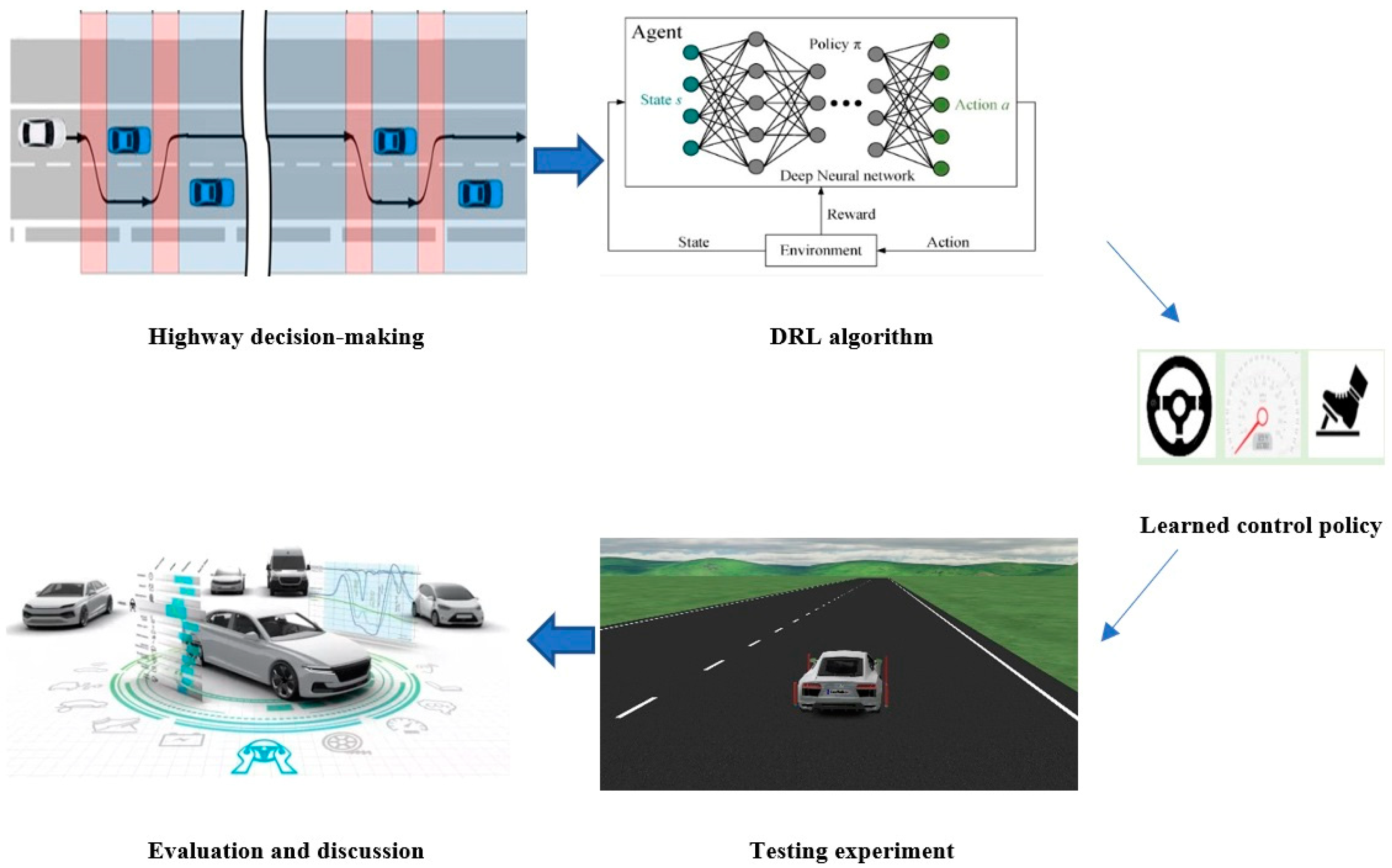
The approach is personalized for continuous action horizons in highway scenarios, as shown in Figure 1.

Based on Figure 1, highway decision making is performed by the powerful DRL method, which means the DDPG algorithm. To accomplish this purpose, the driving environment will be simulated in the Carmaker simulator, while the DDPG algorithm learns the driving actions like steering angle and accelerating or decelerating.

The study begins by defining the real vehicle dynamic in [22] and driving scenarios by the Carmaker scenario [22] to ensure the automated vehicle operates safely and efficiently. The DDPG-enhanced DRL method leverages the actor–critic method to directly obtain control actions, establishing a trust region with clipped objectives. The DRL algorithm’s implementation details are elaborated upon in the subsequent sections. Finally, the performance of the decision-making algorithm for a specific scenario including lane change, double lane change, and lane keeping is evaluated, and, also, for different scenarios, the algorithm adaptability is validated. This paper presents three key innovations that aim to improve the safety and efficiency of AD on highways for real maneuvering. These contributions are as follows:

• Development of an advanced, safe, and efficient decision-making policy for AD on highways for a real maneuver using the DDPG algorithm;
• Using real vehicle dynamics and real scenarios in the Carmaker simulator.

To elaborate on these contributions, this paper is structured as follows:

Section 2 provides a description of vehicle dynamics and driving scenarios on highways. Section 3 details the research on DDPG-enhanced DRL. Also, Section 4 evaluates the simulation results relevant to the presented decision-making strategy. Finally, concluding remarks are presented in Section 5.

2. Vehicle Dynamic and Driving Scenario

This section outlines the testing scenario for highway driving, which includes the autonomous ego vehicle (AEV) and the other vehicles on the road. It also describes the vehicle dynamics of the AEV involved. Additionally, reference models for driving maneuvers in the CarMmaker simulator are introduced.

2.1. Vehicle Dynamic

This study utilized the vehicle dynamics framework in the commercial multi-body simulation IPG CarMmaker as presented in [22].

2.2. Driving Scenario

This study involves creating a driving scenario in the CarMmaker simulator with three lanes per direction of travel. The objective is to simulate real-world driving conditions on the highway. An AEV will navigate through the scenario by ascertaining the control actions for vehicle speed and steering angle at each time step. The AEV aims to travel as swiftly as possible while ensuring safety on the road and avoiding collisions with surrounding vehicles. The ultimate goal of the AEV is to reach the highway exit (Figure 2).

Typically, three criteria are commonly employed to assess the effectiveness of decision-making policies: safety, efficiency, and comfort. Safety entails ensuring that the AEV avoids collisions. Efficiency suggests that the AEV aims to enhance speed. Comfort entails regulating the lane-changing frequency and the extent of deceleration of the vehicle. In this study, the main priorities for the AEV are safety and efficiency. The vehicle typically positions itself in the fast lane, as depicted in Figure 3. The AEV is represented by the white vehicle, while the other vehicles represent the surrounding traffic. Each lane has different types of traffic. In this context, an episode refers to the AEV overtaking all adjacent vehicles to reach its destination on the highway. To ensure simplicity and versatility, we assume that the highway has three lanes (N = 3). Each lane contains different surrounding vehicles. The autonomous vehicle (AEV) is programmed to drive in the right lane. The simulation runs at a frequency of 20 Hz, with the AEV making decisions every second (sampling time of 1 s). Each episode lasts for 50 s. The driving behavior of the adjacent vehicles is governed by random models including autonomous vehicles and human driver vehicles.

3. RL Method

One of the sub-items of artificial intelligence (AI) is machine learning (ML), aiming to develop computational algorithms performance with data. Machine learning (ML) is classified into three main types: reinforcement learning (RL), supervised learning, and unsupervised learning. In the RL method, by trying to maximize a predefined reward function, an autonomous agent learns to fulfill a task in an environment. When the agent opts for a desirable action when interacting with its environment, it is rewarded. In contrast, a punishment or a negative reward is assigned to the autonomous agent, if the selected action is undesired.

Supervised learning concisely involves learning from labeled examples from experts. Since finding a label that exactly denotes an interaction is complicated, the approach is not appropriate for solving interactive problems [24].

As unsupervised learning, the method is learning to find a hidden configuration in unlabeled data. Though finding construction in collected data through learning is useful, the approach cannot optimize a reward, which is an objective of the RL [24].

Some RL problems have huge numbers of states and actions in the environment. In these RL problems, an artificial neural network (ANN) can be used as a function approximator. Utilizing an ANN as a function approximator in RL is called the deep reinforcement learning (DRL) method. The RL problems are typically depicted as Markov decision processes (MDPs). An MDP is a mathematical structure employed to represent decision-making challenges where results are influenced by both random factors and the decisions made by an agent. This framework finds extensive application in fields such as RL and operations research.

The key components of a Markov decision process are as follows:

States (S): The states of MDPs represent all possible situations or configurations of the environment. These states can be discrete or continuous, depending on the problem domain.

Actions (A): For each state in the MDP, there is a range of potential actions that the decision making can take. Actions represent the choices or decisions available to the decision making at each state.

Transition Probabilities (P): The transition probabilities ascertain the likelihood of transitioning from one state to another after executing a particular action. In other words, they specify the likelihood distribution across potential next states given the current state and action.

Rewards (R): At each state–action pair, there is an associated reward that represents the immediate benefit or cost of taking that action in that state. Rewards can be positive (rewards) or negative (penalties), and they may be deterministic or stochastic.

Policy (π): A policy is a mapping from states to actions, specifying the decision maker’s strategy for selecting actions at each state. Reinforcement learning algorithms often strive to discover an optimal policy that maximizes the expected total reward over time.

Value Function (Q): The value function signifies the anticipated total reward achievable by adhering to a specific policy or executing a particular action within a given state. It helps in evaluating the quality of different policies or actions.

MDPs satisfy the Markov property, which implies that the subsequent state relies solely on the current state and action, not on the history of previous states and actions. This property simplifies the modeling and analysis of decision-making problems and allows for the application of various solution techniques, encompassing dynamic programming, Monte Carlo methods, and temporal difference learning.

Markov decision processes supply a formal framework for studying decision making under uncertainty and are widely used in areas such as robotics, autonomous systems, game theory, economics, and more.

The expected discounted reward R_t after the t time step can be considered as:

$${\mathrm{R}}_t={\sum }_t^{\infty }{\mathsf{\gamma }}^t·r_t$$

(1)

where, when γ is in the range [0, 1], it is a discount factor. Parameter t, depending on the problem, is the finite value. Also, policy π (a|s) maps from states to action probabilities. ${\mathrm{V}}^{\mathsf{\pi }}\left(\mathrm{s}\right)$ can be recognized as an expected return regarding policy π from state s and is a value function and it is as follows:

$${\mathrm{V}}^{\mathsf{\pi }}\left({\mathrm{s}}_t\right)={\mathrm{E}}_{\mathsf{\pi }}\left[{\mathrm{R}}_t\right|{\mathrm{S}}_t,\mathsf{\pi }]$$

(2)

${\mathrm{Q}}^{\mathsf{\pi }}\left(\mathrm{s},\mathrm{a}\right)$ is an action-value function as follows:

$${\mathrm{Q}}^{\mathsf{\pi }}\left({\mathrm{s}}_t,{\mathrm{a}}_t\right)={\mathrm{E}}_{\mathsf{\pi }}\left[{\mathrm{R}}_t\right|{\mathrm{S}}_t,{\mathrm{a}}_t,\mathsf{\pi }]$$

(3)

The iterative Bellman equation is satisfied:

$${\mathrm{Q}}^{\mathsf{\pi }}\left({\mathrm{s}}_t,{\mathrm{a}}_t\right)={\mathrm{E}}_{\mathsf{\pi }}\left[{\mathrm{r}}_t+\mathsf{\gamma } \max \left({\mathrm{Q}}^{\mathsf{\pi }}\left({\mathrm{s}}_{t+1},{\mathrm{a}}_{t+1}\right)\right)\right]$$

(4)

However, not all RL problems can be formulated as MDP. In specific situations, if state S can only be observed partly from the environment or cannot be observed directed from the defined environment, then our problems are able to be formulated as a partially observable Markov decision process (POMDP) for such events. A way to solve the problem is to produce observations that include past knowledge by containing previous observations or prior information together with a current observation and therefore solve the problem as an MDP. Learning a policy that maximizes the expected return is the main objective of the RL algorithm.

3.1. Deep Deterministic Policy Gradient (DDPG)

The deep deterministic policy gradient (DDPG) algorithm [24] is a reinforcement learning algorithm that combines elements of both value-based and policy-based methods. It is particularly well-suited for addressing problems with continuous action spaces in reinforcement learning.

DDPG utilizes an actor–critic architecture in which there are two main networks:

• Actor network: This network learns the policy function, which maps states to actions. It aims to maximize the expected return by directly selecting actions based on the current state;
• Critic network: This network learns the value function, which approximates the expected return (cumulative reward) of following a particular policy. It helps to evaluate the actions chosen by the actor network.

Also, DDPG is an off-policy algorithm, meaning it learns from data sampled from an experience replay buffer without explicitly following a specific policy. It is also model free, meaning it does not involve knowledge of the underlying dynamics of the environment. Unlike some other algorithms that are more suited to discrete action spaces, DDPG is designed to handle continuous action spaces, making it applicable to a wide range of problems, including robotics and control tasks.

A mean-squared Bellman error (MSBE) is defined as:

$$\mathrm{L}\left(\mathrm{\varnothing },\mathsf{\theta }\right)={\mathrm{E}}_D\left[{({\mathrm{Q}}_{\varnothing }\left(\mathrm{s},\mathrm{a}\right)-\left(\mathrm{r}+\mathsf{\gamma }\left(1-\mathrm{d}\right)\mathrm{m}\mathrm{a}\mathrm{x}{\mathrm{Q}}_{\varnothing }\left(\acute{\mathrm{s}},\acute{\mathrm{a}}\right)\right))}^2\right]$$

(5)

The DDPG algorithm combines elements of policy gradient methods and Q-learning. The actor network is trained using policy gradient methods to directly maximize the expected return, while the critic network is trained using Q-learning to approximate the value of state–action pairs.

In addition, DDPG introduces target networks to stabilize training. These are copies of the actor and critic networks that are updated less frequently than the main networks. Additionally, DDPG utilizes an experience replay buffer to store and sample experiences during training (based on Figure 4). This helps to decorate the data and improve sample efficiency.

Also, the reward function is as follow:

$${\mathrm{R}}_{\mathrm{t}}=0.5\left|\mathsf{\theta }\right|+0.1\left|\mathrm{a}\right|-\mathrm{c}\mathrm{o}\mathrm{l}\mathrm{l}\mathrm{i}\mathrm{s}\mathrm{i}\mathrm{o}\mathrm{n}+\mathrm{M}$$

(6)

where θ is the steering angle, a is longitudinal acceleration, and collision is 1, if d_relative = 0, and M is a constant.

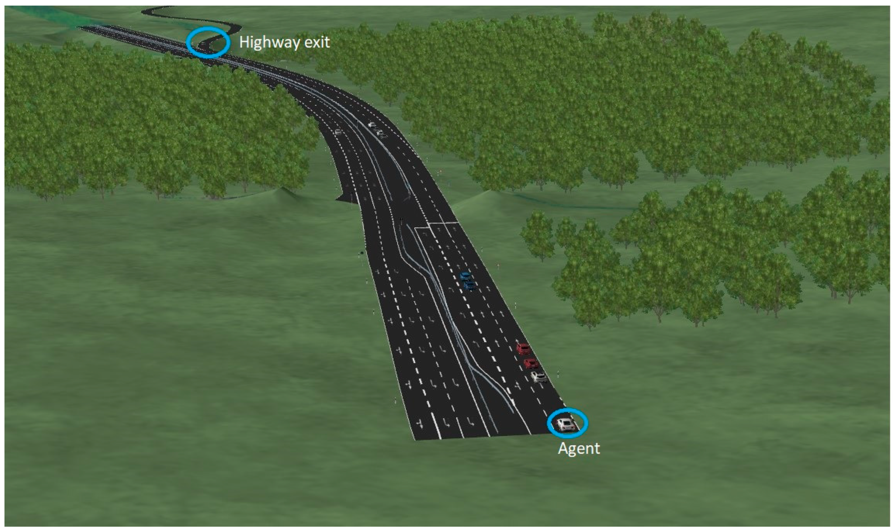
Based on Equation (6), the agent is trained in the highway environment to cross the highway exit.

3.2. Deep Q-Network (DQN)

The Deep Q-network (DQN) algorithm is a deep reinforcement learning technique that integrates Q-learning with deep neural networks to approximate the optimal action-value function in a continuous state space. The DQN operates by learning to map states to actions directly from raw sensory inputs, typically images, enabling it to handle high-dimensional input spaces. It uses experience replay and a target network for stabilizing training and preventing over fitting by storing and randomly sampling past experiences from a replay buffer and periodically updating a target network with the weights of the trained Q-network. Through iterative updates using gradient descent, the DQN aims to minimize the temporal difference error between the forecasted Q-values and the target Q-values, ultimately learning a policy that maximizes cumulative rewards in the environment.

4. Discussion

This section assesses the performance of a proposed decision-making strategy for the AEV using the deep deterministic policy gradient (DDPG) method. The evaluation covers three main aspects. Firstly, it compares and verifies the efficacy of this decision-making approach against an alternative method using detailed simulation outcomes to demonstrate its superiority. Secondly, it validates the DDPG algorithm’s learning capability by examining the accumulated rewards. Lastly, it assesses the derived decision-making strategy in two comparable driving scenarios on the highway to showcase its adaptability.

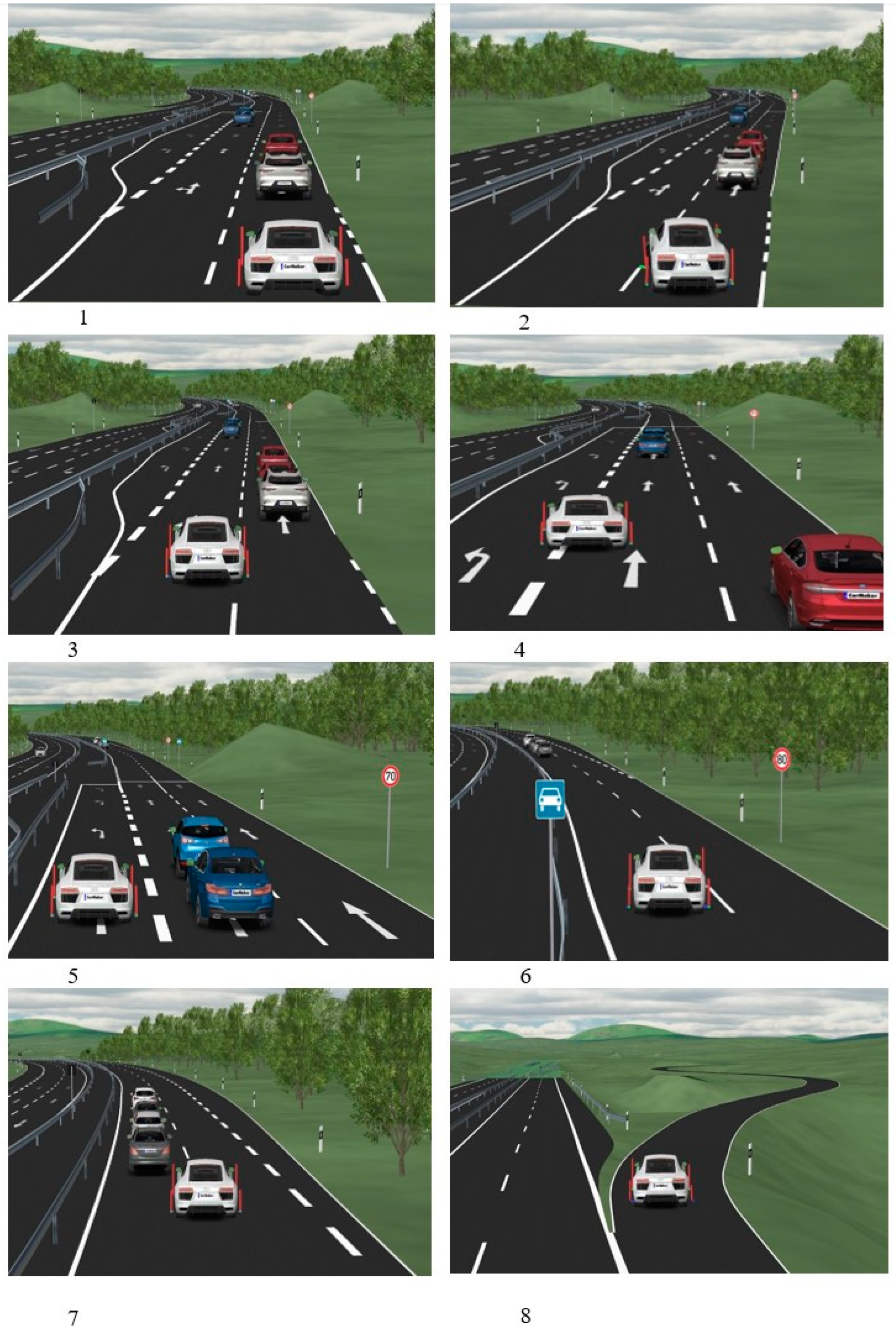
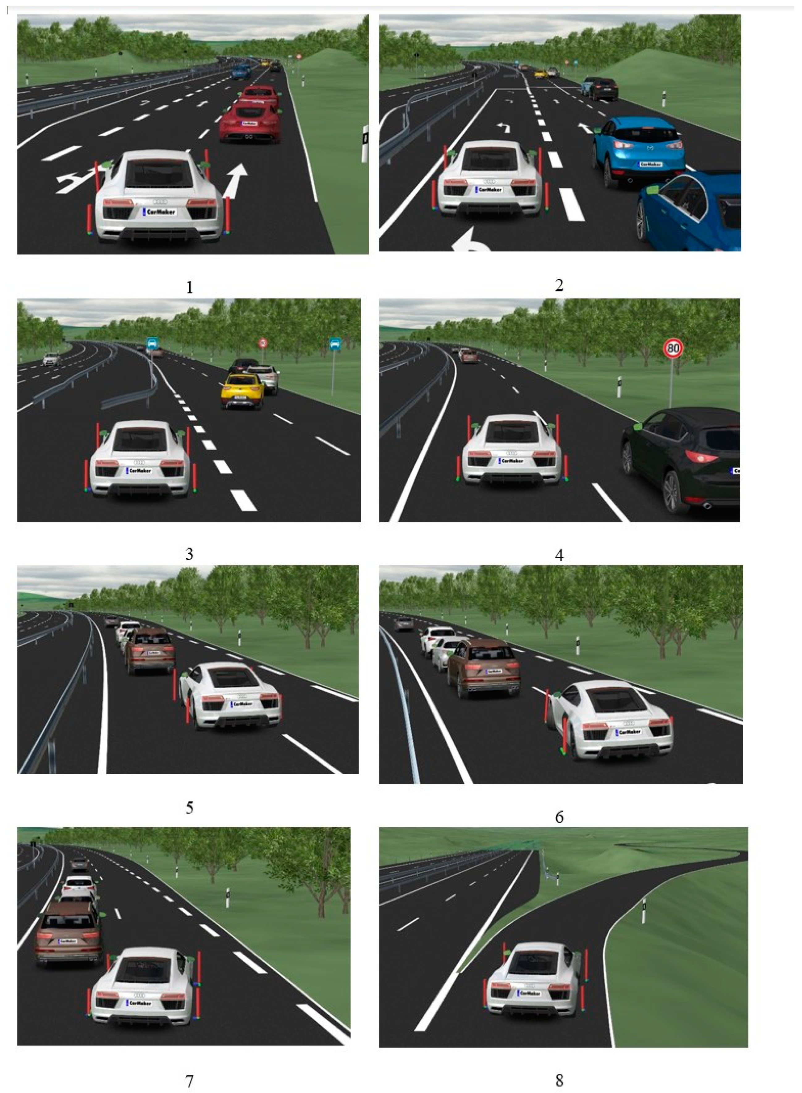
Figure 5 illustrates the specific scenario performed by the DDPG agent in the CarMmaker simulator.

4.1. Performance Evaluation

In this section, we are comparing the performance of DDPG and the DQN, both of which employ a hierarchical control framework. However, the upper levels differ. The default parameters for both DDPG and the DQN are identical. Figure 6 and Figure 7 display the average rewards and episode rewards obtained by the DDPG and DQN agents, respectively. According to Figure 6 and Figure 7, a higher reward signifies, when driving on the preferred lane, more efficiently maneuvering.

The DDPG approach exhibits superior training stability and learning speed than the DQN approach (based on

Table 1. Comparative analysis of DDPG and DQN algorithms.

Parameter	DDPG	DQN
Max episode reward	892	791
Max average reward	443	355
Max speed (m/s)	16.9	14.7
Max distance (m)	961	907

), resulting in consistently higher rewards after approximately 1000 episodes. The main reason why DDPG is considered superior is due to the actor–critic network it uses. These networks can calculate the value of the chosen action at each step, allowing the ego vehicle to quickly identify a better decision-making policy.

To analyze the trajectories of the state variable in this study, Figure 8 displays the average vehicle speed for DDPG and DQN agents for 200 s.

A high speed means that the ego vehicle can maneuver through the driving environment more quickly, resulting in the acquisition of greater total rewards. Also, higher average vehicle speed indicates that the DDPG agent has learned a better policy for controlling the vehicles in the environment. This could suggest that the DDPG algorithm is more effective in this particular scenario for maximizing speed-related objectives. In other words, DDPG is an actor–critic algorithm that utilizes deterministic policy gradients. It tends to be more sample efficient and stable than the DQN.

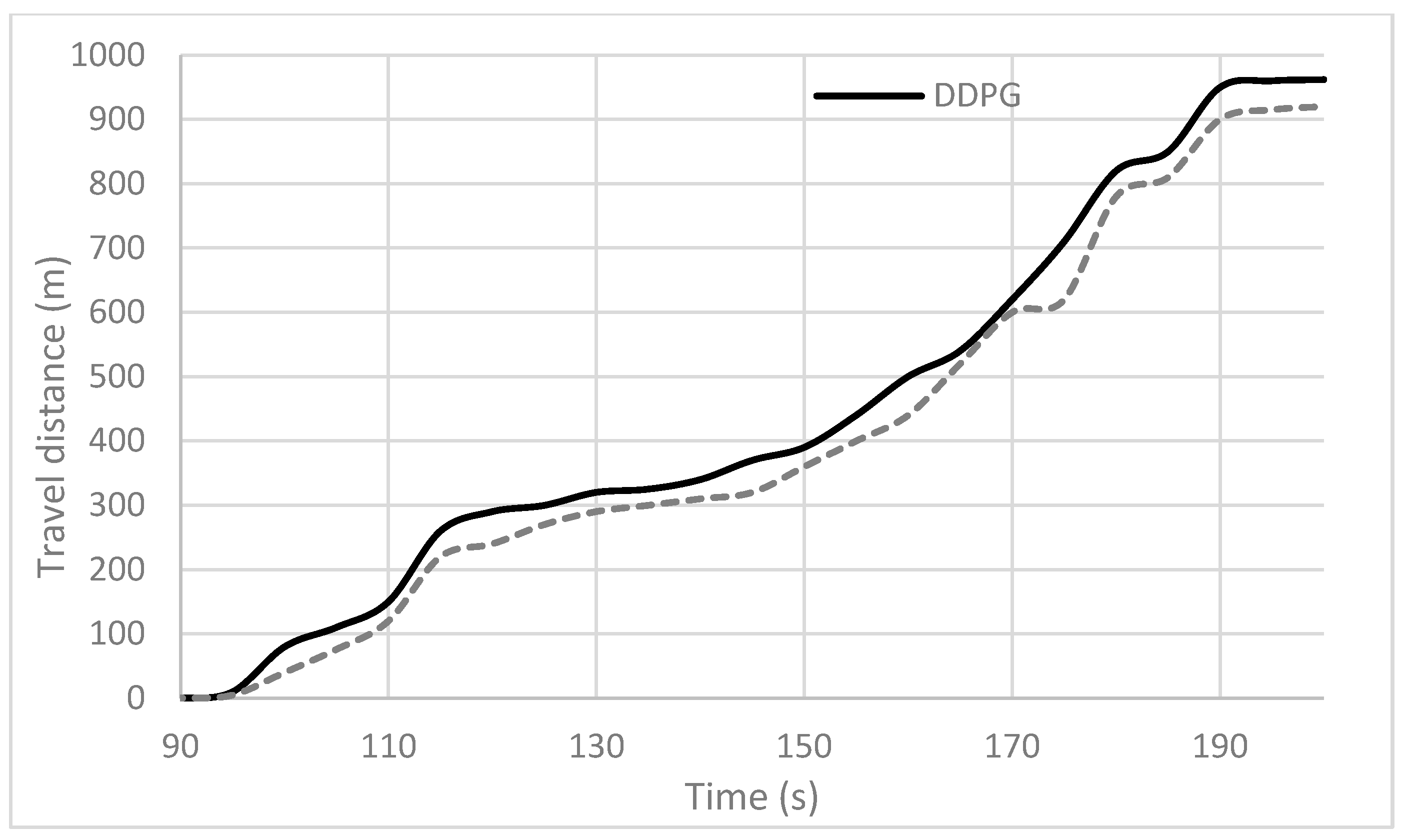
The greater travel distance achieved by the DDPG agent suggests that it navigated the environment more efficiently than the DQN agent (based on Figure 9). This indicates that the DDPG agent made better use of its actions and state information to move through the environment, avoiding unnecessary delays or detours. Also, DDPG’s continuous action space allows for more nuanced control over the agent’s actions compared with the DQN’s discrete actions. This finer-grained control has enabled the DDPG agent to select actions that result in smoother, more continuous movement, facilitating longer travel distances.

As mentioned earlier, DDPG often requires fewer samples to learn compared with the DQN. If DDPG achieved higher speeds and greater travel distances, it indicates that DDPG has learned a more effective policy more efficiently than the DQN in this particular scenario. In addition, the combination of higher average speeds and greater travel distances demonstrates that the DDPG agent outperformed the DQN agent regarding overall movement efficiency and effectiveness in the environment. This indicates that DDPG may be better suited for tasks where minimizing travel time is important.

The differences observed in the performance of the decision-making policies in this study were highlighted by the trajectories displayed. These results indicate that the policy proposed in this study outperforms the DQN benchmark methods. The superiority of the decision-making strategy enabled by DDPG is evident when considering all the results presented in this subsection, as it achieved successful episodes consistently.

4.2. Criticality Evaluation

According to Figure 5, part 7, the DDPG agent has a near condition for collision; then, we consider criticality metrics as follows:

To calculate the time to collision (TTC) in this scenario, we use the following formula:

$${\mathrm{T}\mathrm{T}\mathrm{C}}_{low}=\mathrm{m}\mathrm{i}\mathrm{n}({\displaystyle \frac{∆\mathrm{X}\left(\mathrm{t}\right)}{∆\mathrm{V}\left(\mathrm{t}\right)}})$$

(7)

where

Agent velocity (v_agent) = 2.8 m/s

Distance to the static vehicle (d) = 4.4 m

The relative velocity (v_relative) in this case would be the sum of the agent’s velocity and the static vehicle’s velocity (since it is not moving):

v_relative = v_agent − 0 = 2.8 m/s − 0

v_relative = 2.8 m/s

Now, we can calculate TTC based on (6):

$${\mathrm{T}\mathrm{T}\mathrm{C}}_{low}={\displaystyle \frac{4.4}{2.8}}=1.57\mathrm{s}$$

(8)

So, the ${\mathrm{T}\mathrm{T}\mathrm{C}}_{low}$ in this scenario is approximately 1.57 s.

A time to collision (TTC) of 1.57 s indicates that there is still a reasonable (based on UN regulation No. 157 [26]) amount of time before a potential collision occurs between the agent and the static vehicle.

Figure 10 shows the behavior of the calculated TTC(t) according to Equation (6) in the presented scenario (based on Figure 5, parts 6–7), when following a target vehicle. We observe the lowest value for TTC at 1.57 s, a mean value of 2.89 s., and a standard deviation of 0.90 s when approximated with Gaussian behavior. Typically, autonomous emergency braking (AEB) systems include an intervention strategy that warns the driver if the TTC falls below approximately 2.5 s and initiates partial braking at approximately 1.5 s. Full braking would be applied at ${\mathrm{T}\mathrm{T}\mathrm{C}}_{low}$ values below 0.6 to 0.8 s. The vehicle manufacturer defines the thresholds of these intervention strategies and is also sometimes adjusted by the driver, changing the setup of the AEB system in the configuration menu of the car. Hence, the algorithm is usually in an acceptable range but sometimes requires braking interventions to stay in a safe area.

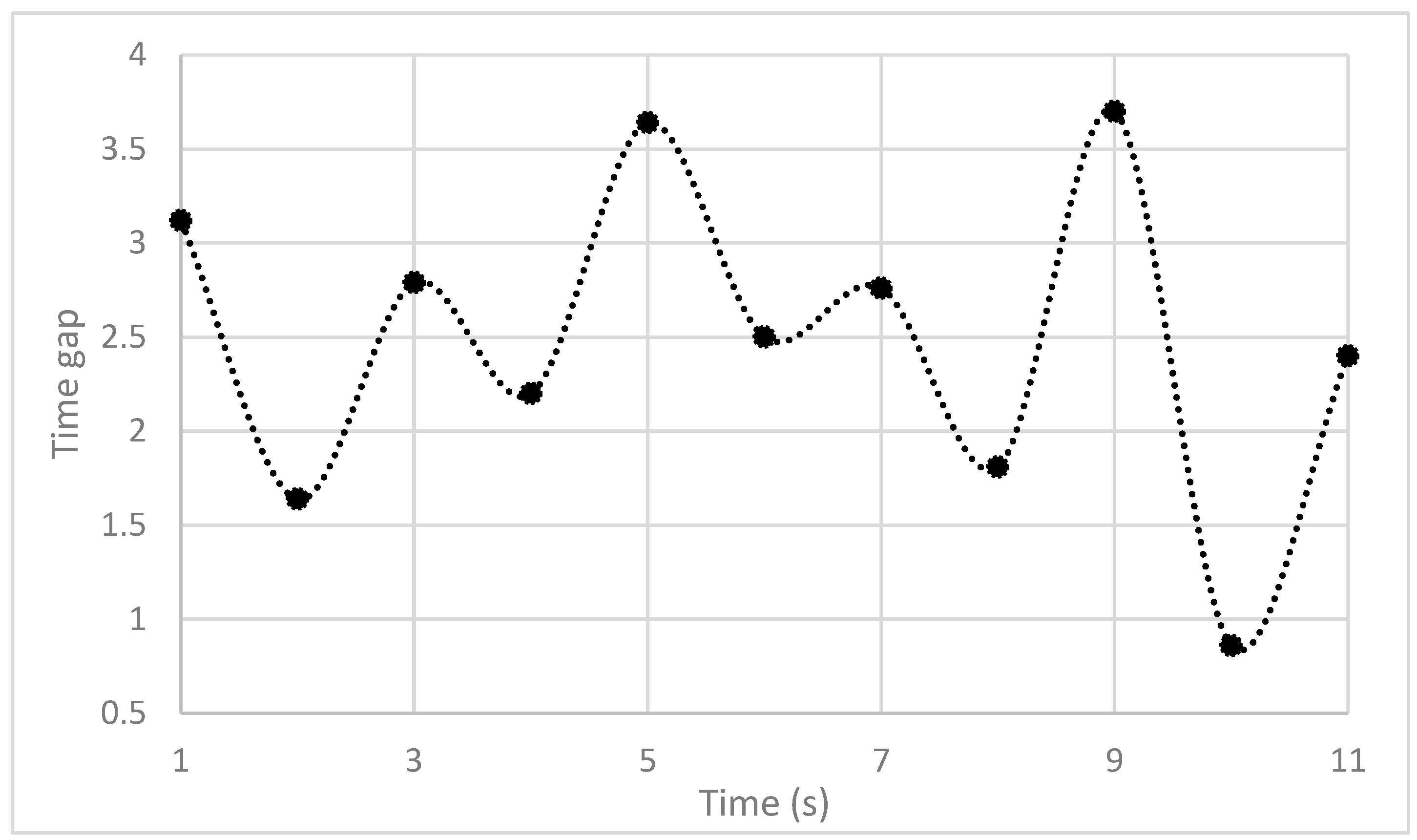
In addition, the time gap between the ego vehicle and the target vehicle was calculated according to the following Equation (8),

$${\mathrm{t}}_{Gap}={\displaystyle \frac{∆\mathrm{X}}{V_{Ego}}}$$

(9)

where, again, $∆\mathrm{X}$ is the relative distance between the target and ego vehicle and $V_{Ego}$ is the ego vehicle speed.

Figure 11 shows the behavior of the time gap during the same scenario (based on Figure 5, parts 6–7). The lowest value reads 0.86 s, the average value is 2.60 s, and the standard deviation is 0.95 s. According to [26], most drivers prefer a time gap of 1.8 s compared with 1.0 and 1.3 s. Hence, we conclude that, in the current setting of the algorithm, the driving scenario is usually uncritical and acceptable for most drivers. A more detailed consideration of criticality is part of future investigations and will include more advanced criticality metrics as compared with the TTC. TTC is limited to the constant relative velocity between the target and ego vehicle and therefore not always suitable for criticality evaluation.

4.3. Comparison between DDPG and DQN

This experiment evaluates the DDPG and DQN algorithms, both established techniques in deep reinforcement learning (DRL), to determine their effectiveness in learning and training methods.

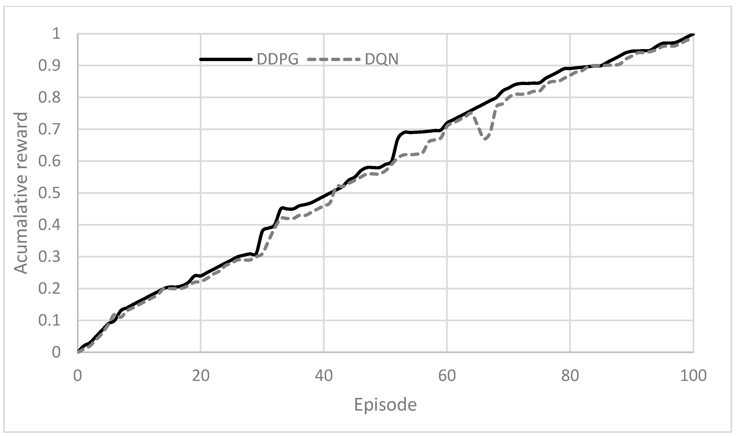
To demonstrate how the dueling network can be applied to future decisions in AD, Figure 12 displays the trajectory of cumulative rewards for 100 episodes.

According to Figure 12, higher cumulative rewards indicate that the DDPG agent’s learned policy was more effective at maximizing rewards in the environment compared with the DQN agent. This suggests that DDPG was able to make better decisions over time, leading to higher overall rewards. Also, DDPG’s continuous action space and deterministic policy gradients may have allowed it to optimize its policy more efficiently than the DQN. This could have enabled the DDPG agent to explore and exploit the state–action space more effectively, leading to higher cumulative rewards.

In other words, DDPG’s ability to learn a deterministic policy and its actor–critic architecture has enabled it to consider the long-term consequences of its actions better than the DQN. This has contributed to its ability to accumulate higher rewards over time. Moreover, DDPG’s deterministic policy gradients have provided a more stable learning process compared with the epsilon-greedy exploration strategy used in the DQN. This has allowed DDPG to learn a more optimal policy with less variance, leading to higher cumulative rewards.

Figure 12 shows a decreasing trend, which indicates that both ego vehicles are becoming more acquainted with the driving environment as they interact with it. Moreover, the DDPG algorithm can gain a greater understanding of traffic situations in the same number of episodes, resulting in a faster learning process. As a result, the ego vehicle can navigate more efficiently and safely with the guidance of the DDPG algorithm.

4.4. Adaptability Estimation

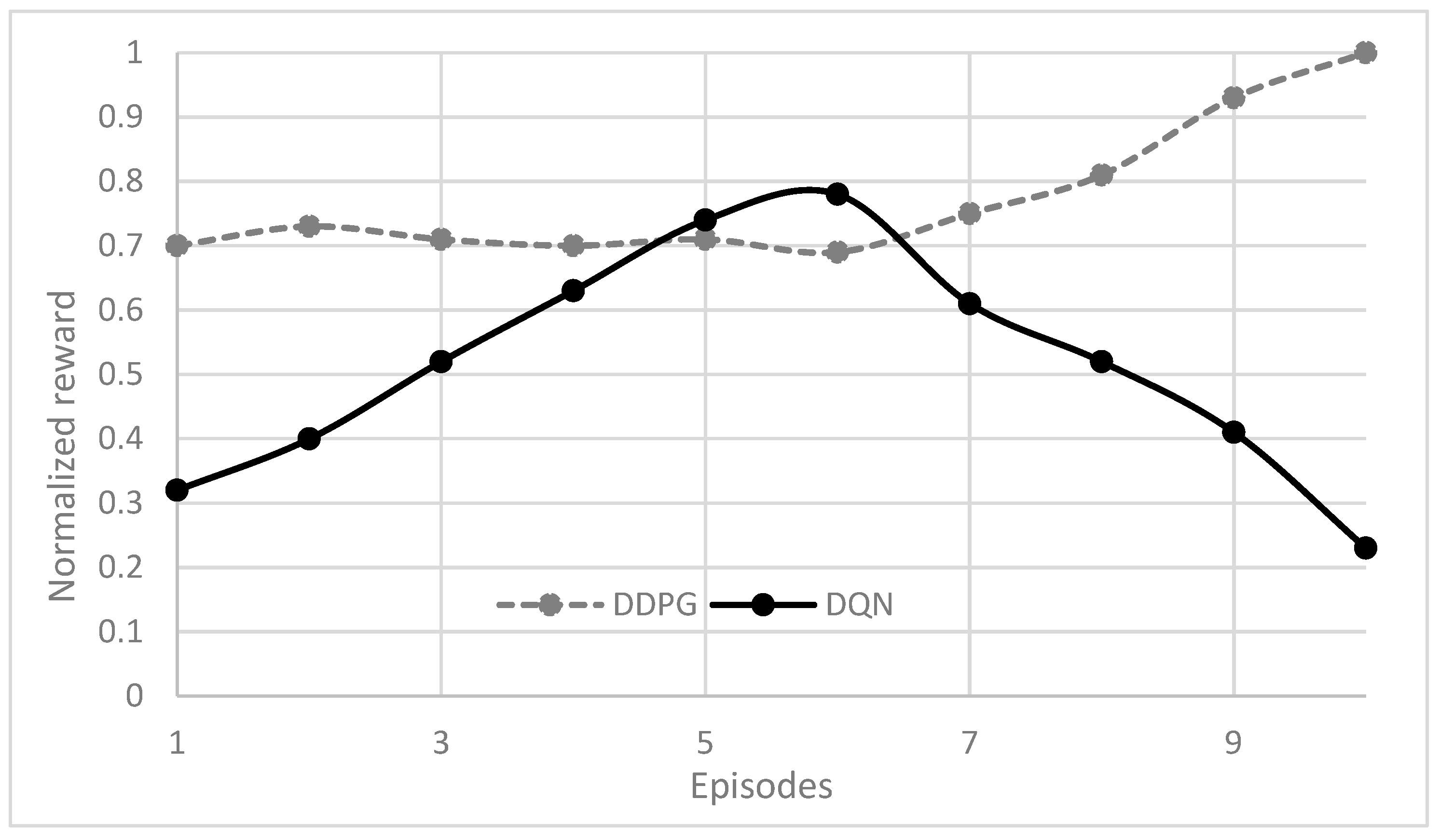
After training automated vehicles for highway driving scenarios, a phase is implemented to evaluate their ability to adapt. The testing phase consists of 10 episodes with the initial configurations remaining consistent with the training phase. The neural networks’ parameters acquired during training are preserved and can be directly applied in new circumstances. During testing, the average reward achieved and instances of collisions are analyzed to ensure that the vehicles can adapt to new situations. During the testing phase, Figure 13 shows the normalized average reward achieved by the DDPG and DQN methods. The reward is mainly determined by the vehicle’s speed and collision occurrences.

The average reward might not reach its maximum score of 100 in this study due to instances where the ego vehicle must decelerate to prevent collisions. Additionally, the ego vehicle may need to switch lanes to facilitate overtaking maneuvers. To illustrate decision-making performance, three representative situations (A and B indicated in Figure 14 and Figure 15) are selected for analysis without loss of generality.

Figure 14 demonstrates a driving scenario where the ego vehicle is surrounded by three vehicles in front of it. The ego vehicle needs to engage in extended car-following maneuvers until it finds an opportunity to overtake them. Consequently, the vehicle may not achieve its maximum speed, and it might not surpass all surrounding vehicles before reaching its destination.

Moreover, Figure 15 depicts an uncommon driving scenario where the ego vehicle attempts a risky lane change to gain higher rewards. Then, due to insufficient operating space, it overtakes nearby vehicles while it has minimum speed. These kinds of occurrences are infrequent during training and can potentially lead the ego vehicle to cause collisions.

The comprehensive analysis presented in Figure 14 and Figure 15 suggests the need for further refinement of the adaptable decision-making strategy through extended training. These findings also underscore the applicability of the corresponding control policy in real-world settings.

The DDPG algorithm succeeded in two different scenarios tested; it indicates a high level of adaptability and generalization ability.

The fact that DDPG performed well across multiple scenarios suggests that it was able to generalize its learned policy effectively. Generalization refers to the capability of an algorithm to apply knowledge gained from one scenario to perform well in new, unseen scenarios. DDPG’s success in two scenarios indicates that it learned a policy that is robust and applicable across a range of environments. Moreover, DDPG’s success in diverse scenarios highlights its flexibility as a reinforcement learning algorithm. It was able to adapt its policy to different environmental conditions and task requirements, demonstrating its ability to handle varying complexities and dynamics. DDPG’s success across multiple scenarios also reflects its learning dynamics, including exploration strategies, update rules, and memory mechanisms. These learning dynamics have enabled DDPG to efficiently learn and adapt its policy to different environmental conditions.

Eventually, DDPG’s consistent success across different scenarios also presents its robustness as an algorithm. Robustness refers to an algorithm’s ability to maintain good performance despite variations in the environment or perturbations in the learning process. DDPG’s ability to perform well in diverse scenarios suggests that it is robust to changes and uncertainties.

5. Conclusions

The study employs DRL techniques to explore the challenge of highway decision making. In this study, we introduce an innovative approach by incorporating a unique combination of driving scenarios, specifically lane change, double lane change, and lane keeping, which have not been collectively utilized in prior studies. This combination allows for a comprehensive evaluation of the decision-making DDPG algorithm under varied and complex driving conditions. By addressing this complex scenario, the present study offers a more realistic testing framework, enhancing the reliability adaptability of AD systems in real-world situations. This innovation not only fills a gap in the existing research but also contributes to the advancement of safer and more efficient AD technologies. A tailored control framework is established using the DDPG algorithm within the driving environments to ensure safety and effectiveness. The paper presents the proposed approach’s performance, convergence rate, and adaptability through a sequence of simulation experiments. According to the results, the DDPG algorithm is more efficient and safer than the DQN technique. Furthermore, the testing results are thoroughly evaluated, showcasing the potential of the proposed approach to be successfully implemented in real-world driving scenarios. Future work involves implementing online highway decision making via hardware-in-loop research and using real-world highway databases to estimate relevant overtaking strategies.