Abstract
The moving particle simulation (MPS) method is a simulation technique capable of calculating free surface and incompressible flows. As a particle-based method, MPS requires significant computational resources when simulating flow in a large-scale domain with a huge number of particles. Therefore, improving computational speed is a crucial aspect of current research in particle methods. In recent decades, many-core CPUs and GPUs have been widely utilized in scientific simulations to significantly enhance computational efficiency. However, the implementation of MPS on different types of hardware is not a trivial task. In this study, we present an implementation method for the explicit MPS that utilizes the Taichi parallel programming language. When it comes to CPU computing, Taichi’s computational efficiency is comparable to that of OpenMP. Nevertheless, when GPU computing is utilized, the acceleration of Taichi in parallel computing is not as fast as the CUDA implementation. Our developed explicit MPS solver demonstrates significant performance improvements in simulating dam-break flow dynamics.
1. Introduction
Simulating free surface flow is important in many areas of engineering and science, including civil and environmental engineering, naval architecture, oceanography, and hydrology. Accurate simulations of free surface flow can provide valuable information for the design of structures and infrastructure that interact with water, such as dams, levees, and offshore platforms. Grid-based methods, such as the finite difference method (FDM), lattice Boltzmann method (LBM), and finite volume method (FVM), are commonly used to simulate free surface flow [1,2,3,4,5,6]. These methods divide the domain into a grid or mesh and solve the governing equations for the flow variables at each grid point. However, these grid-based methods have difficulties in simulating free surface flow with large deformations or fragmentation due to numerical errors or instabilities arising from the interface capturing schemes.
Recently, the mesh-free or Lagrangian method, such as the smoothed particle hydrodynamics (SPH) method [7], has been attracting attention because it is very efficient in solving problems involving large deformations and free surfaces [8,9]. Similarly to SPH, the MPS method [10,11] is also a Lagrangian mesh-free method that solves the Navier–Stokes equations by tracking the movement of fluid particles. The method divides the fluid domain into particles that are assigned properties such as mass, velocity, and pressure. These properties are then updated at each time step by solving the governing equations for each particle. Both methods can be used to simulate compressible and incompressible flows, and they have undergone relevant improvements in stability and accuracy [12,13,14,15].
The main limitation of MPS is that it can be computationally expensive and requires a large number of particles to accurately capture the flow behavior. To overcome this limitation, the parallel computing technique can be used to improve its efficiency and make it feasible for practical applications [16,17,18]. As a massively parallel processor, the GPU can achieve high accelerations and efficiency using CUDA or OpenCL programming frameworks [19,20]. However, writing codes using these frameworks requires a high level of programming skill as well as the knowledge of the hardware architectures [21,22]. On the other hand, the recently developed Taichi framework is designed with a focus on enabling high-performance numerical computation, particularly on modern hardware architectures like GPUs. Taichi is designed with the aim of improving the efficiency of implementing high-performance computing which requires a holistic approach that considers the entire system, including the programming language, the hardware architecture, and the optimization algorithms [23,24,25,26]. One of the main merits of Taichi is its ability to take full advantage of modern hardware, including GPUs, by providing a high-level language that can be efficiently compiled to machine code. This ability can lead to significant accelerations over traditional approaches. Moreover, Taichi’s syntax is intentionally crafted to resemble Python, facilitating a swift adoption for developers already acquainted with Python. Additionally, Taichi stands out as a user-friendly option for newcomers interested in numerical computing due to its relatively low learning curve, distinguishing it from other programming languages. From an academic perspective, Taichi has been used in a variety of research projects, including simulations of fluid dynamics, molecular dynamics, image processing, and machine learning [27,28,29]. Overall, Taichi’s combination of high-performance, flexibility, ease of use, and active community makes it a promising language for high-performance numerical computing, particularly on modern hardware architectures.
In this paper, we aim to use the Taichi programming language to accelerate the explicit moving particle simulation (EMPS) method and test the performance of parallel computing on both the CPU and GPU. Evaluations of efficiency and accuracy using the Taichi framework are carried out carefully. Based on our investigation, the Taichi framework exhibits robust potential for accelerating particle simulation. The unique features of the Taichi framework, such as its ability to operate on both CPU and GPU architectures and its support for parallel computations, enhance the speed and efficiency of flow simulations.
2. Explicit MPS Method
The EMPS was proposed by Koshizuka et al. [10,11] to simulate free surface flow. In the conventional semi-implicit MPS method, a Poisson equation derived from the incompressible condition should be solved to calculate the pressure field. Although solving the Poisson equation improves the simulation accuracy and ensures the overall incompressibility, it suffers a high computational cost. On the other hand, the EMPS method explicitly calculates all terms of the following Navier–Stokes equations
where P, , , t, , and represent pressure, density, flow velocity, time, kinematic viscosity, and gravitational acceleration, respectively. In the EMPS method, the pressure is calculated by the equation of state (EOS) [13,30,31]:
In the above EOS, is used [32], and c is the artificial speed of sound. The sound speed must be ten times as large as the maximum fluid velocity to limit the density fluctuation for a nearly incompressible condition. is the relative density, which can be calculated from the particle number density defined in Equation (5).
In the MPS method, fluids are discretized by Lagrangian particles, where the flow variables in terms of velocity and pressure are defined. The following weight function is used for spatial discretization and calculating the derivatives of physical quantities [11]
where r is the distance between two particles and represents the influence radius. To ensure computational stability and efficiency, it is recommended that the influence radius be 2–4 times the initial particle distance [16]. For particle i, the particle number density can be defined as
where and represent the coordinates of particles i and j, respectively [33]. The fluid density is considered to be proportional to the particle number density.
The velocity viscosity term and the pressure gradient term in the governing Equation (1) can be discretized as follows [10]:
where d represents the number of dimensions, is the constant particle number density and is a constant parameter equal to weighted average of the squares of the distances to neighboring particles in the influence radius. Particles in EMPS method are usually categorized into fluid particles (blue) and stationary wall particles (black) (Figure 1). The value of constant is determined for particle which in the fluid part at the initial state of the calculation. The same value of is used for all particles. During the simulation, remains constant. is the minimum value among the pressure at particle and the pressure in its neighboring particles.
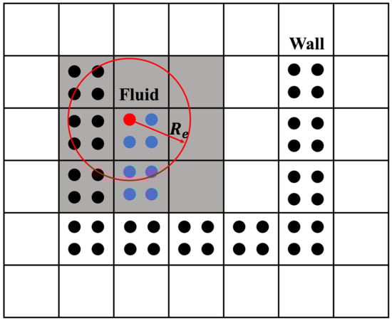
Figure 1.
Particles and buckets of the EMPS method (blue: fluid particles; black: wall particles; red: current calculating particle; gray: buckets within interaction domain; : influence radius).
In the EMPS method, an intermediate step is needed to achieve time discretization. The intermediate velocity and pressure of the particle can be updated as follows:
The intermediate step is represented by *, and k means the present time step. The variables of time step can be calculated as follows:
Once the particle velocities and coordinates have been corrected, it is necessary to recalculate the particle number density at the next time step based on the updated coordinates.
To maintain numerical stability, the artificial sound speed should be slower than the sound speed of the actual physical property [32]. The numerical stability condition is determined by the Courant number using the flow velocity and the Courant number using the sound velocity :
where is the maximum value of the flow velocity and represents the distance between particles. The upper limit 0.2 for and 1.0 for are obtained from a numerical experiment.
The Dirichlet boundary condition is implemented by computing the particle number density using Equation (5). If the calculated density surpasses the constant particle number density , the particle is identified as internal, and the pressure is calculated. Conversely, if the density is below the reference value, it is considered a free surface particle, and its pressure is set to zero [32]. To impose a non-slip boundary condition on the wall during viscosity calculations, it is essential to impart an opposite velocity to the wall particles [34]. This ensures that the velocity on the surface of the wall is zero. Alternatively, we can set the velocity of the wall particles to zero, which may introduce a slight error in the viscous term near the wall.
The EMPS method can use the bucket technique to enhance the computational efficiency [19,35,36,37]. By partitioning the domain into a series of buckets (Figure 1), each of which accommodates a cluster of particles, particle interactions can be solely computed among the particles residing in the same or neighboring buckets. This approach significantly mitigates the computational expense associated with the algorithm, primarily by reducing the searching process during the calculation of the particle interactions. This feature is particularly critical for large-scale simulations, where the computational expense of searching becomes prohibitively high.
The procedure of an EMPS method is summarized below in Figure 2. After setting the initial states of each particle, the calculation for each time step begins. First, the gravity and viscosity terms are calculated explicitly, and then the intermediate particle velocities and coordinates are updated. After the particles are moved, the intermediate pressure is explicitly calculated using the adjusted particle coordinates. After calculating the pressure gradient, we modify the velocity and coordinates of the particles. The updated particle coordinates are then used to correct the intermediate pressure. If a particle is found to have moved outside the boundary, it will be classified as a ‘GST’ type and excluded from subsequent calculations. After this step, the coordinates, velocity, and pressure of each particle at the new time can all be obtained.
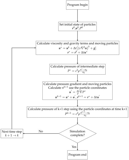
Figure 2.
The flowchart of EMPS method.
3. Implementation of EMPS Using Taichi
In this part, we present the Taichi implementation of the MPS method. The Taichi framework is a versatile high-performance computing framework tailored for applications in computer graphics, computational physics, and computational science, offering seamless integration with Python to balance ease of use with computational efficiency. It is designed to excel in various hardware environments by supporting multiple backends, including CPUs and GPUs across different manufacturers, ensuring broad accessibility and optimal performance. Key features include the automatic optimization and parallelization of code, dynamic scheduling for adaptively handling computational workloads, and built-in support for sparse computations and differentiable programming. These features make the Taichi framework a powerful tool for developers and researchers working on a wide range of computational tasks, from fluid dynamics simulations to molecular dynamics simulations. In Taichi framework, setting ‘arch=ti.cpu’ in ‘ti.init’ function specifies the use of CPU. The ‘cpu_max_num_threads’ parameter regulates the maximum number of CPU cores that the program can utilize. Changing the arch argument in the ‘ti.init’ function to either ‘ti.gpu’ or ‘ti.cuda’ will enable Taichi to utilize the GPU for simulation. In this study, the fast math function in the ‘ti.init’ is disabled to prevent precision loss problems.
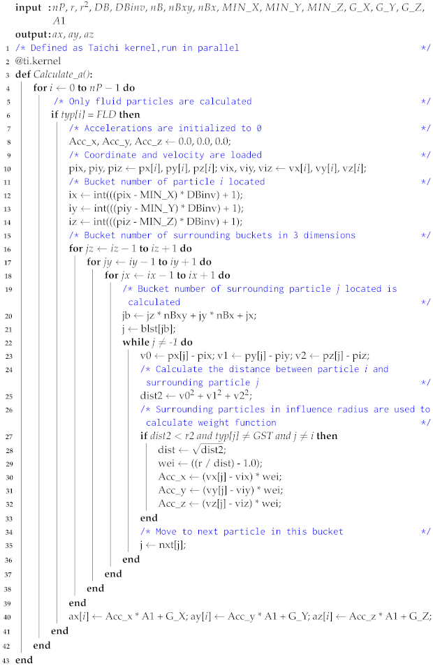
To parallelize a function in Taichi, it is sufficient to decorate the function with ‘@ti.kernel’. The kernel serves as the fundamental execution unit in Taichi. It is worth noting that only the outermost loop will be executed in parallel. As shown below in Algorithm 1, only the outermost for loop in line 4 will be parallelized, so placing the most computationally intensive loop at the outermost level of the function can significantly enhance the performance of the Taichi program. Since the EMPS method uses particles as the object of computation, the outermost for the loop in the program is usually set to traverse all particles. It can be expected that Taichi is effective for simulations with a large particle number.
Multiple kernels can be defined within the same Taichi program, and these kernels are independent of each other. The order of execution of the kernels depends on the sequence in which they are first called. Once a kernel is compiled, it is cached, reducing the startup overhead when the kernel is called multiple times within the same program. In this EMPS code, functions such as‘Calculate_a’, ‘Calculate_p’, ‘Pressure_gradient’, ‘Move’ are defined as kernels. They are used to calculate the acceleration, pressure, pressure gradient, and movement of particles, respectively.
In this simulator, the ‘Check_position’ function, responsible for verifying whether particles exceed the boundaries, is decorated with ‘@ti.func’, which is a Taichi function that can be invoked by a kernel. The ‘Check_position’ Taichi is then utilized in the ‘Move’ kernel. Particle positions, velocities, pressures, and other physical quantities are stored in a Taichi field format. In Taichi, the field serves as a global data container. Data can be passed between the Taichi scope and Python scope through a field. At the same time, using field to store data also allows Taichi to achieve the continuous arrangement of data and improve the memory usage efficiency.
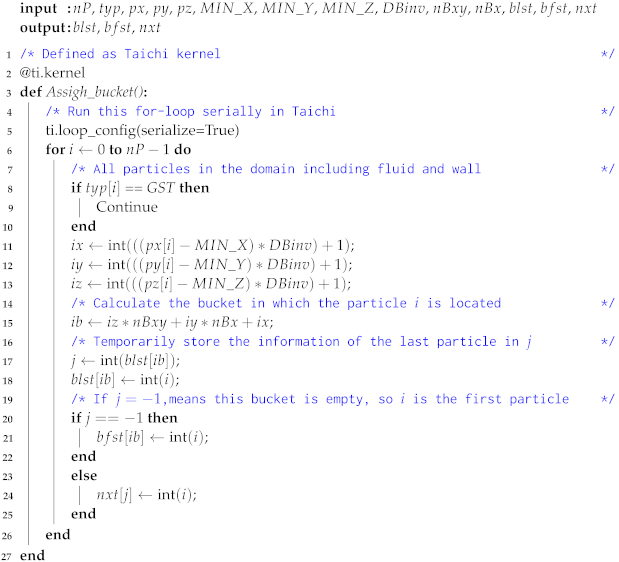
In Taichi, part of the program can run serially when necessary to prevent errors. As presented in Algorithm 2, ‘bfst’ is an array storing the index of the first particle in each bucket, ‘blst’ contains the index of the last particle in each bucket, and ‘nxt’ holds the indices of the next particles in the same bucket. As indicated in line 15, ‘blst[ib]’ is temporarily stored in ‘j’ to check whether the bucket ‘ib’ contains any particles. In this algorithm, the particles are sorted in a bucket starting from the first index ‘bfst’ and ending at the last index ‘blst[ib]’ in a sequential manner. The next particle index ‘nxt’ is determined one by one. Therefore, if this process is parallelized, it can lead to inconsistencies in the information stored in ‘bfst’, ‘blst’, and ‘nxt’. Then, ‘ti.loop_config(serialize=True)’ is added to the function so that Taichi will run it serially. This ensures the particle indices stored in the buckets are correct.
| Algorithm 1: Taichi kernel used to calculate acceleration |
 |
| Algorithm 2: Bucket method in EMPS |
 |
4. Numerical Benchmark
Two classical free-surface problems were simulated using our developed Taichi-EMPS solver. The computation times using the Taichi platform were compared to those of serial computing, and a detailed analysis of the performance improvement was conducted. Furthermore, the accuracy of the simulation was evaluated by comparing it with other numerical methods [38].
4.1. Dam Break Flow
The dam-break benchmark is a commonly used test to simulate free surface flows. This involves simulating the scenario where a partially filled tank with water suddenly ruptures, allowing the water to flow out of the tank and form waves and other complex surface features. In this test, a tank with dimensions of 1.0 × 0.2 × 0.6 m is used, with an open roof and the right side of the tank closed by a gate. The simulation is initialized with a water level of 0.5 m to mimic the dam-break process. To accurately calculate the pressure distributions, three layers of wall particles are utilized. For this simulation, we chose a particle spacing of 0.02 m. The total number of particles, which includes both water and wall particles, is 19,136. An analysis of spatial resolution is presented in Appendix A. Decreasing the distance between particles has a significant impact on both the total number of particles and the computational workload. The following section will discuss the relationship between particle spacing and the computational time.
We conducted a 1 s dam-breaking simulation with a time interval of s, determined by Equations (14) and (15). The results of the simulation, depicting the motion of the water column at different time steps, are illustrated in Figure 3. To assess the precision of the results, we compared the position of the front tip of the water on the bottom surface with the experimental data and other numerical results in Figure 4 [38,39,40]. Our analysis indicates that the EMPS method yields simulation results that are closer to the experimental values, compared to other numerical techniques [38].
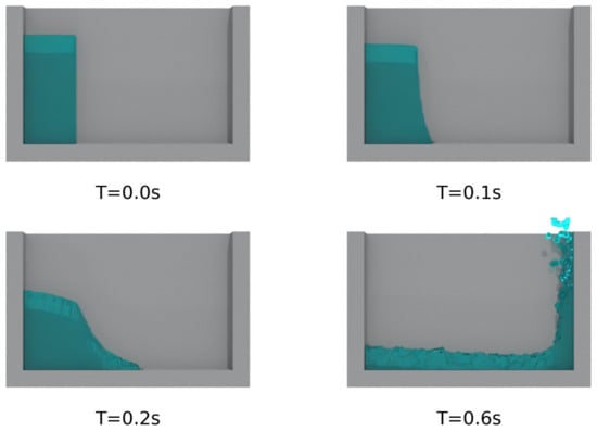
Figure 3.
Simulation results of a simple dam break flow at different time steps.
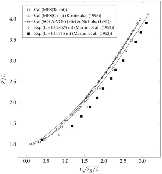
Figure 4.
Comparisons of the temporal variations of the water tip’s position at the bottom during the dam break (Z: distance of water tip from vertical plane; L: a dimension characteristic of the water column base; : dimensionless time) [38,39,40].
To evaluate Taichi’s computational efficiency, we compared the computation times using different codes with different types of implementations (Native Python 3.9.0, C++ 20, OpenMP 5.2, and CUDA 11.0). The computational time for the dam break simulation case is 200.51 s for serial computation using Taichi 1.0.4, compared to 200.14 s using C++. Therefore, it has sped up the Python code 237 times and achieved the same computational efficiency as C++ code in the case of serial computation.
Subsequently, we conducted an investigation to evaluate the computational efficiency of the Taichi programming language using GPU (GeForce RTX 3060 Ti, NVIDIA, Santa Clara, CA, USA) and multicore CPU (INTEL Core i5 9400F, Intel, Santa Clara, California, USA), in conjunction with various parallel programming libraries (i.e., OpenMP and CUDA). As Taichi has been designed to be optimized for both CPU and GPU architectures, our initial comparison focused on the computational time of parallel CPU and GPU computing in the Taichi platform. In terms of parallel CPU computation time, we observed that the efficiency of Taichi is nearly identical to that of OpenMP. According to the results shown in Table 1, the computation time for CPU (six cores) and GPU was 38.87 s and 23.58 s, respectively, demonstrating an acceleration of only 1.65 times with GPU usage. This can be attributed to the modest particle number in the benchmark test case, which limited the CUDA cores (computing units in GPUs) from functioning at full capacity. In contrast, the computation time using CUDA implementation was 9.64 s, indicating much greater efficiency compared to Taichi GPU computing, as the CUDA implementation features finely tuned optimizations for local calculations. It is worth noting that our study only parallelized the primary loop for traversing all particles in the Taichi code. Further optimization and tuning could potentially enhance the code efficiency, particularly for complex computations. For example, optimizing the use of Taichi inline functions ‘ti.func’ is recommended to reduce the function call overhead. Another possible recommendation is to replace the nested for-loop with a single, flat for-loop.

Table 1.
The calculation time for various programming languages and implementation strategies.
4.2. Dam Break Impact on a Solid Obstacle
To demonstrate the robustness of our Taichi-EMPS solver, we also conducted a flow simulation to emulate the intricate behavior of fluid flows when a dam breaks and encounters an obstacle in its path [41]. In this simulation, a 3.22 m long open tank with a 1 × 1 cross-section was employed, and 0.55 m of water was introduced with a gate placed to seal the right side of the tank (Figure 5). An obstacle measuring 40 cm in length and 16 × 16 in cross-section was placed on the left side of the tank, and the distance between the obstacle and the left wall of the tank was set at 0.67 m. In Figure 5, four snapshots of the simulation are presented. After the gate opening, the dam break wave spreads over the downstream area and hits the block obstacle approximately at time t = 0.4 s. To provide further quantitative validation of the accuracy of our results, we measured the time evolution of the water height at designated locations, specifically H4 and H2 (Figure 5). The results are generally consistent with previous simulations [41] and the experimental data from Maritime Research Institute Netherlands (MARIN), as depicted in Figure 6. The minor disparities observed in the results are likely attributed to potential inaccuracies in the process of reconstructing the surface from the particle data.
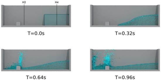
Figure 5.
Simulation results of dam break simulation with a solid obstacle.
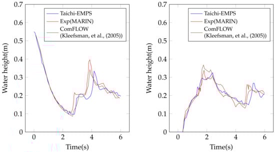
Figure 6.
Comparisons of temporal variations of vertical water heights at H4 (left) and H2 (right) [41].
Next, we conducted an examination on the relationship between acceleration and particle number utilizing this specific scenario. A higher quantity of particles contributes to a more enhanced simulation resolution. We specifically altered the initial particle spacing to be 0.04 m, 0.03 m, and 0.02 m, consequently yielding particle numbers of 36,014, 68,505, and 181,298, respectively. The simulations were executed for a total duration of 8.0 s in physical time, using a time step of s. The acceleration was determined through the ratio of serial to parallel computational times. The computation times and acceleration for the three cases with a different particle number utilizing CPU and GPU-based parallel computing are presented in Figure 7 and Table 2. The acceleration of GPU parallel computing is directly proportional to the number of particles, highlighting the scalability of the GPU-based Taichi solver. However, the acceleration of CPU parallel computing roughly remained constant when we increase the particle number. This discrepancy can be attributed to the limited number of cores used on the CPU (only six), in contrast to the 4864 CUDA cores available on the GPU. When the number of particles is increased, the large amount of GPU’s CUDA cores are more effectively employed, leading to a higher computational performance. Therefore, the GPU parallel computing is more efficient when operating on a large number of particles.
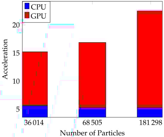
Figure 7.
Relationship between the particle number and acceleration for CPU and GPU.
Table 2.
The computation times of CPU and GPU-based parallel computing.
Then, we focused on examining the efficiency of Taichi CPU parallel computing by using more CPU cores (up to 16 cores of Ryzen 9 7950X CPU, AMD, Santa Clara, California, USA). The acceleration when increasing the used CPU cores was quantified by simulating a fixed-scale system with a substantial particle count of 68,505 (strong scaling). In this large-scale system, we can observe that the acceleration increased with the increase in CPU cores (Figure 8 (left)). Nevertheless, it is noteworthy that the relationship between the number of employed CPU cores and the resulting acceleration is not strictly linear. The acceleration leveled off when we raised the CPU core from 15 to 16. Amdahl’s law [42] states that the acceleration of a computer program depends on the proportion of its serial portion. Even if the parallel portion of the program can be accelerated infinitely, the overall acceleration is limited by the serial portion. Therefore, Amdahl’s law provides the theoretical upper limit of the acceleration for parallel computing, which is expressed as:
where P represents the proportion of a program that can be made parallel (functions decorated by ‘@ti.kernel’), and N represents the number of processors used. In this study, the proportion P is calculated based on the execution time for the parallelizable and non-parallelizable part of the program using one CPU core. The P value of our Taichi-EMPS solver is 0.998, which means the most of the program was parallelized. Amdahl’s law indicates that as the number of processors used increases, the acceleration gradually decreases until it reaches a limit. Thus, to maximize computational performance, it is crucial to minimize the serial portion of the program as much as possible. Compared with the ideal acceleration determined by Amdahl’s law, our simulation acceleration was very close to the upper limit when CPU core number is below 10 (Figure 8 (left)). However, the gap between the simulation acceleration and the ideal value became larger when more CPU cores are used because of the marked increase in communication time for the transmission of particle information among CPU cores in configurations employing a large number of cores.
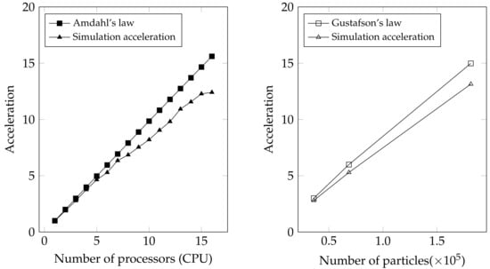
Figure 8.
Parallel efficiency evaluations by strong scaling (left) and weak scaling (right) tests. The simulation accelerations are compared with the ideal values according to Amdahl’s law (left) and Gustafson’s law (right).
Another key concept in parallel computing is Gustafson’s law [43], in which the ideal acceleration can be defined as:
By increasing both the workload and the processors, the scalability can be maintained (weak scaling). Therefore, we increased the number of CPU cores used while also increasing the particle number to examine the acceleration in the weak scaling scenario. Figure 8 (right) shows the results of weak scaling acceleration for particle numbers of 36,014, 68,505, and 181,298 using 3, 6, and 15 cores, respectively. As the particle number and CPU cores increase, the simulation acceleration exhibits a linear increase but below the ideal value. The reason may also be attributed to the increase in communication time when the core number is large.
5. Conclusions
In this study, we present an efficient EMPS solver, implemented in the Taichi programming language to facilitate parallel computing. This solver takes advantage of the EMPS method and the Taichi programming language, resulting in a significant acceleration of numerical simulations for free surface flow. To validate the solver’s efficiency and accuracy, we conducted a classical dam break simulation. It was found that the original Python code can be accelerated by more than 237 times using Taichi programming language, approaching the efficiency level of the C++ code. Moreover, the ability to seamlessly switch between CPU and GPU computing can be achieved by selecting a single parameter to alter the architecture. While comparing the rate enhancement of CPU and GPU parallel computing with different particle numbers, it has emerged that the superiority of GPU parallel computation extends to scenarios involving an immense number of particles. Nevertheless, the efficiency of GPU computation using the Taichi programming language exhibited a noticeable gap when compared to CUDA. Finally, our developed Taichi-EMPS solver demonstrated notable performance in simulating the free surface flow problem and exhibits compatibility with cross-platform systems.
Author Contributions
Conceptualization, F.J. and Y.Z.; methodology, F.J. and Y.Z.; software, Y.Z.; validation, Y.Z.; formal analysis, F.J. and Y.Z.; investigation, F.J. and Y.Z.; resources, F.J.; data curation, Y.Z.; writing—original draft preparation, Y.Z.; writing—review and editing, Y.Z., F.J., and S.M.; visualization, Y.Z.; supervision, F.J.; project administration, S.M.; All authors have read and agreed to the published version of the manuscript.
Funding
This research was partially supported by JSPS KAKENHI Grant Number JP22K03927.
Data Availability Statement
The Taichi-EMPS is open source under MIT License and available in the Github repository at https://github.com/laiyinhezhiying/taichi-EMPS-solver (accessed on 16 January 2024).
Conflicts of Interest
The authors declare no conflicts of interest.
Appendix A. Grid-Independent Test
To guarantee that the particle spacing does not impact the simulation results, a grid-independent test was conducted. To examine the impact of spatial resolution on the migration of the water tip, we conducted a dam-break simulation by altering the particle spacing, ranging from 0.01 m to 0.1 m. The findings depicted in Figure A1 indicate that there are only slight variations when the particle spacing is adjusted between 0.02 and 0.04 m. Decreasing the particle spacing to 0.01 m does not significantly improve the accuracy of the outcomes. However, when the spacing between particles is adjusted to 0.1 m, there was a notable deviation in the position of the water tip, and the liquid particles were unable to reach the opposite end within a time frame of 0.004 s. Therefore, we consider it suitable to set the spacing between particles at 0.02, 0.03, and 0.04 m.
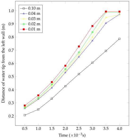
Figure A1.
Grid-independent test for particle spacings of 0.01, 0.02, 0.03, 0.04, and 0.10 m.
References
- Tomé, M.F.; Mangiavacchi, N.; Cuminato, J.A.; Castelo, A.; Mckee, S. A finite difference technique for simulating unsteady viscoelastic free surface flows. J. Non–Newton. Fluid Mech. 2002, 106, 61–106. [Google Scholar] [CrossRef]
- Casulli, V. A semi-implicit finite difference method for non-hydrostatic, free-surface flows. Int. J. Numer. Methods Fluids 1999, 30, 425–440. [Google Scholar] [CrossRef]
- Muzaferija, S.; Perić, M. Computation of free-surface flows using the finite-volume method and moving grids. Numer. Heat Transf. 1997, 32, 369–384. [Google Scholar] [CrossRef]
- Jiang, F.; Matsumura, K.; Ohgi, J.; Chen, X. A GPU-accelerated fluid–structure-interaction solver developed by coupling finite element and lattice Boltzmann methods. Comput. Phys. Commun. 2021, 259, 107661. [Google Scholar] [CrossRef]
- Jiang, F.; Yang, J.; Boek, E.; Tsuji, T. Investigation of viscous coupling effects in three-phase flow by lattice Boltzmann direct simulation and machine learning technique. Adv. Water Resour. 2021, 147, 103797. [Google Scholar] [CrossRef]
- Jiang, F.; Liu, H.; Chen, X.; Tsuji, T. A coupled LBM-DEM method for simulating the multiphase fluid-solid interaction problem. J. Comput. Phys. 2022, 454, 110963. [Google Scholar] [CrossRef]
- Gingold, R.; Monaghan, J. Smoothed Particle Hydrodynamics - Theory and Application to Non-Spherical Stars. Mon. Not. R. Astron. Soc. 1977, 181, 375–389. [Google Scholar] [CrossRef]
- Dalrymple, R.; Rogers, B. Numerical modeling of water waves with the SPH method. Coast. Eng. 2006, 53, 141–147. [Google Scholar] [CrossRef]
- Hu, X.; Adams, N. A multi-phase SPH method for macroscopic and mesoscopic flows. J. Comput. Phys. 2006, 213, 844–861. [Google Scholar] [CrossRef]
- Koshizuka, S.; Nobe, A.; Oka, Y. Numerical Analysis of Breaking Waves using the Moving Particle Semi-implicit Method. Int. J. Numer. Methods Fluids 1998, 26, 751–769. [Google Scholar] [CrossRef]
- Koshizuka, S.; Oka, Y. Moving-Particle Semi-Implicit Method for Fragmentation of Incompressible Fluid. Nucl. Sci. Eng. 1996, 123, 421–434. [Google Scholar] [CrossRef]
- Cummins, S.J.; Rudman, M. An SPH projection method. J. Comput. Phys. 1999, 152, 584–607. [Google Scholar] [CrossRef]
- Shakibaeinia, A.; Jin, Y.C. A weakly compressible MPS method for modeling of open-boundary free-surface flow. Int. J. Numer. Methods Fluids 2010, 63, 1208–1232. [Google Scholar] [CrossRef]
- Tayebi, A.; Jin, Y.C. Development of moving particle explicit (MPE) method for incompressible flows. Comput. Fluids 2015, 117, 1–10. [Google Scholar] [CrossRef]
- Jandaghian, M.; Shakibaeinia, A. An enhanced weakly-compressible MPS method for free-surface flows. Comput. Methods Appl. Mech. Eng. 2020, 360, 112771. [Google Scholar] [CrossRef]
- Murotani, K.; Masaie, I.; Matsunaga, T.; Koshizuka, S.; Shioya, R.; Ogino, M.; Fujisawa, T. Performance improvements of differential operators code for MPS method on GPU. Comput. Part. Mech. 2015, 2, 261–272. [Google Scholar] [CrossRef]
- Gou, W.; Zhang, S.; Zheng, Y. Implementation of the moving particle semi-implicit method for free-surface flows on GPU clusters. Comput. Phys. Commun. 2019, 244, 13–24. [Google Scholar] [CrossRef]
- Khayyer, A.; Gotoh, H. Enhancement of performance and stability of MPS mesh-free particle method for multiphase flows characterized by high density ratios. J. Comput. Phys. 2013, 242, 211–233. [Google Scholar] [CrossRef]
- Green, S. Particle simulation using cuda. NVIDIA Whitepaper 2010, 6, 121–128. [Google Scholar]
- Goodnight, N. CUDA/OpenGL fluid simulation. NVIDIA Corp. 2007, 548, 1–11. [Google Scholar]
- Kim, K.S.; Kim, M.H.; Park, J.C. Development of Moving Particle Simulation Method for Multiliquid-Layer Sloshing. Math. Probl. Eng. 2014, 2014, 350165. [Google Scholar] [CrossRef]
- Yang, Y.H.C.; Briant, L.; Raab, C.; Mullapudi, S.; Maischein, H.M.; Kawakami, K.; Stainier, D. Innervation modulates the functional connectivity between pancreatic endocrine cells. eLife 2022, 11, e64526. [Google Scholar] [CrossRef]
- Hu, Y.; Li, T.M.; Anderson, L.; Ragan-Kelley, J.; Durand, F. Taichi: A language for high-performance computation on spatially sparse data structures. ACM Trans. Graph. 2019, 38, 1–16. [Google Scholar] [CrossRef]
- Hu, Y.; Anderson, L.; Li, T.M.; Sun, Q.; Carr, N.; Ragan-Kelley, J.; Durand, F. Difftaichi: Differentiable programming for physical simulation. arXiv 2019, arXiv:1910.00935. [Google Scholar]
- Hu, Y. The Taichi Programming Language: A Hands-on Tutorial. ACM SIGGRAPH 2020 Courses. 2020, 21, 1–50. [Google Scholar] [CrossRef]
- Hu, Y.; Liu, J.; Yang, X.; Xu, M.; Kuang, Y.; Xu, W.; Dai, Q.; Freeman, W.T.; Durand, F. QuanTaichi: A Compiler for Quantized Simulations. ACM Trans. Graph. (TOG) 2021, 40, 1–16. [Google Scholar] [CrossRef]
- Yang, J.; Xu, Y.; Yang, L. Taichi-LBM3D: A Single-Phase and Multiphase Lattice Boltzmann Solver on Cross-Platform Multicore CPU/GPUs. Fluids 2022, 7, 270. [Google Scholar] [CrossRef]
- Wu, Y.C.; Shao, J.L. mdapy: A flexible and efficient analysis software for molecular dynamics simulations. Comput. Phys. Commun. 2023, 290, 108764. [Google Scholar] [CrossRef]
- Dave, S.; Baghdadi, R.; Nowatzki, T.; Avancha, S.; Shrivastava, A.; Li, B. Hardware acceleration of sparse and irregular tensor computations of ml models: A survey and insights. Proc. IEEE 2021, 109, 1706–1752. [Google Scholar] [CrossRef]
- Sun, X.; Sun, M.; Takabatake, K.; Pain, C.; Sakai, M. Numerical Simulation of Free Surface Fluid Flows Through Porous Media by Using the Explicit MPS Method. Transp. Porous Media 2019, 127, 7–33. [Google Scholar] [CrossRef]
- Monaghan, J. Simulating Free Surface Flows with SPH. J. Comput. Phys. 1994, 110, 399–406. [Google Scholar] [CrossRef]
- OOchi, M. Explicit MPS algorithm for free surface flow analysis. Trans. JSCES 2010, 20100013. [Google Scholar] [CrossRef]
- Idelsohn, S.; Oñate, E.; Del Pin, F. The Particle Finite Element Method; A Powerful tool to Solve Incompressible Flows with Free-surfaces and Breaking Waves. Numer. Methods Eng. 2004, 61, 964–989. [Google Scholar] [CrossRef]
- Lee, B.H.; Park, J.C.; Kim, M.H.; Hwang, S.C. Step-by-step improvement of MPS method in simulating violent free-surface motions and impact-loads. Comput. Methods Appl. Mech. Eng. 2011, 200, 1113–1125. [Google Scholar] [CrossRef]
- Mattson, W.; Rice, B.M. Near-neighbor calculations using a modified cell-linked list method. Comput. Phys. Commun. 1999, 119, 135–148. [Google Scholar] [CrossRef]
- Nishiura, D.; Sakaguchi, H. Parallel-vector algorithms for particle simulations on shared-memory multiprocessors. J. Comput. Phys. 2011, 230, 1923–1938. [Google Scholar] [CrossRef]
- Ha, L.; Krüger, J.; Silva, C. Fast 4-way parallel radix sorting on GPUs. Comput. Graph. Forum 2009, 28, 2368–2378. [Google Scholar] [CrossRef]
- Hirt, C.W.; Nichols, B.D. Volume of fluid (VOF) method for the dynamics of free boundaries. J. Comput. Phys. 1981, 39, 201–225. [Google Scholar] [CrossRef]
- Koshizuka, S. A particle method for incompressible viscous flow with fluid fragmentation. Comput. Fluid Dyn. J. 1995, 4, 29. [Google Scholar]
- Martin, J.C.; Moyce, W.J.; Martin, J.; Moyce, W.; Penney, W.G.; Price, A.; Thornhill, C. Part IV. An experimental study of the collapse of liquid columns on a rigid horizontal plane. Philos. Trans. R. Soc. London. Ser. A Math. Phys. Sci. 1952, 244, 312–324. [Google Scholar]
- Kleefsman, K.; Fekken, G.; Veldman, A.; Iwanowski, B.; Buchner, B. A Volume-of-Fluid Based Simulation Method for Wave Impact Problems. J. Comput. Phys. 2005, 206, 363–393. [Google Scholar] [CrossRef]
- Amdahl, G.M. Validity of the single processor approach to achieving large scale computing capabilities. In Proceedings of the Spring Joint Computer Conference, Atlantic City, NJ, USA, 18–20 April 1967; pp. 483–485. [Google Scholar]
- Gustafson, J.L.; Montry, G.R.; Benner, R.E. Development of parallel methods for a 1024-processor hypercube. SIAM J. Sci. Stat. Comput. 1988, 9, 609–638. [Google Scholar] [CrossRef]
Disclaimer/Publisher’s Note: The statements, opinions and data contained in all publications are solely those of the individual author(s) and contributor(s) and not of MDPI and/or the editor(s). MDPI and/or the editor(s) disclaim responsibility for any injury to people or property resulting from any ideas, methods, instructions or products referred to in the content. |
© 2024 by the authors. Licensee MDPI, Basel, Switzerland. This article is an open access article distributed under the terms and conditions of the Creative Commons Attribution (CC BY) license (https://creativecommons.org/licenses/by/4.0/).