Assessing the Impact of Copula Selection on Reliability Measures of Type P(X < Y) with Generalized Extreme Value Marginals

Abstract

In reliability studies, we are interested in the behaviour of a system when it interacts with its surrounding environment. To assess the system’s behaviour in a reliability sense, we can take the system’s intrinsic quality as strength and the outcome of interactions as stress. Failure is observed whenever stress exceeds strength. Taking Y as a random variable representing the stress the system experiences and random variable X as its strength, the probability of not failing can be taken as a proxy for the reliability of the component and given as $P(Y<X)=1-P(X<Y)$. This way, in the present paper, it is considered that X and Y follow generalized extreme value distributions, which represent a family of continuous probability distributions that have been extensively applied in engineering and economic contexts. Our contribution deals with a more general scenario where stress and strength are not independent and copulas are used to model the dependence between the involved random variables. In such modelling framework, we explored the proper selection of copula models characterizing the dependence structure. The Gumbel–Hougaard, Frank, and Clayton copulas were used for modelling bivariate data sets. In each case, information criteria were considered to compare the modelling capabilities of each copula. Two economic applications, as well as an engineering one, on real data sets are discussed. Overall, an easy-to-use methodological framework is described, allowing practitioners to apply it to their own research projects.

1. Introduction

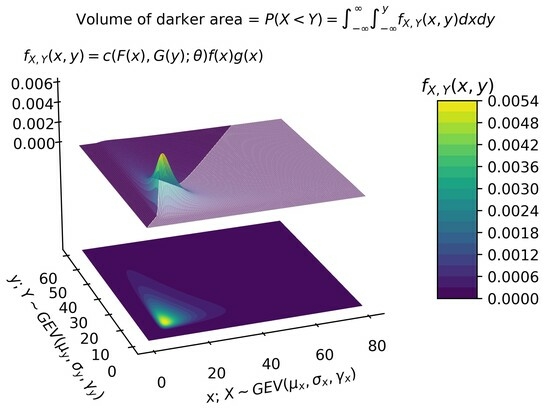
The probability of failure of a system or component can be calculated by statistically comparing the applied stress to its strength. Let X (strength) and Y (stress) be continuous random variables (RVs) with joint probability density function (PDF) $f_{X,Y}(·,·)$. The stress–strength probability (or reliability) is defined as

$$R=P(X<Y)={\int }_{-\infty }^{\infty }{\int }_{-\infty }^y{f}_{X,Y}(x,y)dxdy.$$

(1)

There are several applications of this framework, such as in asset selection [1], household financial fragility [2] and engineering [3], among others. See Kotz et al. [4] for more details.

Equation (1) can only be evaluated when the analytical representation of the joint PDF is known (or any other equivalent statistical formula which can be transformed into $f_{X,Y}$); thus, properly assessing this joint formulation is of utmost importance in stress–strength applications of type $P(X<Y)$. Finding an accurate representation of $f_{X,Y}$ involves two steps: understanding what the marginal distributions are and what the dependence structure of these RVs is.

Thus, at first, finding the best fitting marginal distributions for X and Y is of interest. In this regard, Quetelet’s pioneering investigations, which were focused on finding empirical regularities in biological and social data [5], can be considered to be among the first experimentations of normally distributed (thin-tailed) RVs beyond the pure sciences. Their belief in the universality of the error law had repercussions on the development of 19th century science and statistics. Nevertheless, the experiments involving financial data in the 20th century pointed to the suitability of heavy-tailed distributions in modelling, either by means of $\alpha$-stable processes (heavy-tailed alternative to the thin-tailed Brownian motion [6]) or with heavy-tailed time-series models [7,8]. Although the literature proposes the general hypothesis that logarithmic returns in financial data follow an $\alpha$-stable process with parameter $0<\alpha <2$ [9] (and undefined variance), without loss of generality, results from the extreme value theory (EVT) regarding generalized extreme value (GEV) distributions [10] present these distributions as an alternative to $\alpha$-stable distributions. This approach can be considered valid, since the GEV distribution has fat-tailed behaviour and can be used as a proxy for fat-tailed distributions. From an economic point of view, it is well known that extreme share returns on stock markets can have important implications for financial risk management, and several studies have successfully applied the GEV to model financial data [1,11,12,13,14]. Furthermore, heavy-tailed distributions like log-normal and Pareto are known for their suitability for embracing both the tails and the mode of empirical income density functions [2]. However, some limitations of these distributions give the opportunity to apply other distributions that resemble fat-tailed behaviour but bring more flexibility in the parameter set [15]. Nevertheless, exploring how the GEV distribution performs when modelling income and consumption data in a fragility evaluation framework is still of interest.

Moreover, Kotz and Nadarajah [16] elucidated the characteristics of this distribution, highlighting its broad relevance in various domains, such as accelerated life testing, natural disasters, horse racing, rainfall, supermarket queues, sea currents, wind speeds, track race records, and more. As a result, GEV RVs prove to be suitable models for engineering data sets as well.

After selecting the marginals for X and Y, their dependence structure needs to be considered. The stress–strength reliability when X and Y are independent RVs following extreme distributions has been widely studied in the literature. Nadarajah [17] considered the class of extreme value distributions and derived the corresponding forms for reliability (R) in terms of special functions. Several authors have worked on the estimation and application of stress–strength probability for extreme distributions (e.g., [18,19,20,21]). The stress–strength probability for independent GEV distributions was studied by Quintino et al. [1], who derived stress–strength reliability formulas and investigated the application of the reliability measure $P(X<Y)$ in selecting financial assets with returns modelled by GEV distributions.

To the best of our knowledge, there is no work in the literature addressing stress–strength reliability for dependent GEV distributions. Thus, the main goal of this paper is to extend the approach of [1] by studying (1) when X and Y follow dependent GEV distributions, with the joint PDF being given by copulas. Therefore, our main contributions are:

• To propose an estimation procedure for R and validate such a procedure via a simulation study;
• To apply the estimation procedure on three real-life data sets;
• To present the computational codes needed to implement the methodological framework hereby developed.

Using copulas to model the dependence structure of RVs is a direct consequence of Sklar’s theorem, which enables the creation of several copula families, each of which better captures specific dependence situations. Among the most explored copulas, the Gumbel–Hougaard copula better copes with upper tail dependence among variables. On the other hand, the Clayton copula is well suited for delineating lower tail dependence among variables, while the Frank copula excels at capturing symmetric tail dependence among variables (cf. [22]). For a more detailed study on copula theory, the reader may refer to [23]. Recent works explored copulas in different scenarios, like the use of the Frank copula to model financial assets with Dagum marginals for dependent asset portfolio management [24], the application of copulas in data from insurance companies on losses and expenses [22], the derivation of the bivariate distribution of monsoon rainfall in neighbouring meteorological subdivisions [25], and a monthly streamflow simulation using a maximum entropy–Gumbel–Hougaard copula method [26]. Theoretical properties of extreme value copulas can be also found in [27,28].

Considering their common usage in both financial and engineering applications, Gumbel–Hougaard, Frank, and Clayton copulas are considered in the present paper. Besides theoretical aspects, we explore the estimation procedures, proposing a general framework that can be applied by practitioners while considering GEV marginals with the three types of copula families mentioned. In that case, one may notice that the value of R given in (1) depends on the parameters of the marginal distributions (for GEV distributions, as shall be seen, $\mu$ location, $\sigma$ scale, and $\gamma$ shape) and a dependence parameter, $\theta$ (introduced by the copula model). Motivated by improvement in computational time, we opted for a two-step estimation, i.e., the marginals are modelled, and then the dependence parameter is estimated, which is the so-called method of inference functions for margins [29].

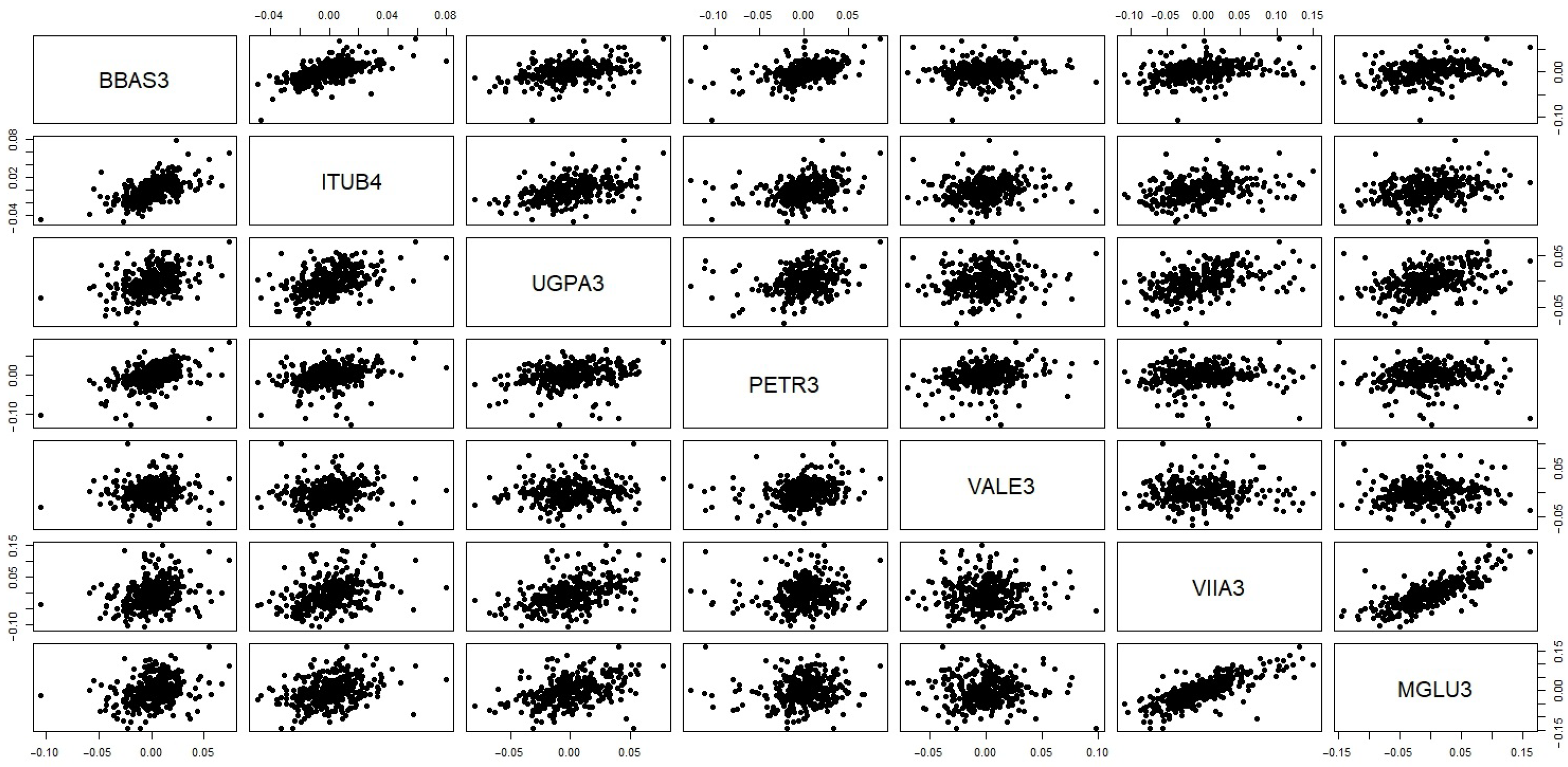
The methodological framework hereby proposed is applied to estimate R in three real situations. Firstly, we consider an asset selection situation where there exists a correlation between the returns of pairs of different stocks. In summary, when X and Y represent financial return random variables and $R<1/2$, it is advisable that the investor chooses the asset corresponding to variable X. If $R>1/2$, the opposite occurs. The case where $R=1/2$ is inconclusive. The measurement of household financial fragility is also considered a second real data set modelling situation. Using data from Bank of Italy’s 2008 Survey on Household Income and Wealth (cf. [2]), we investigate how often households have their yearly consumption higher than their income. Finally, a third database is modelled, allowing one to compare the minimum monthly flow rate for the Piracicaba River in Brazil. Such comparison is useful to define contingency measures to complement the electric matrix, which is mostly dependent on hydraulic sources.

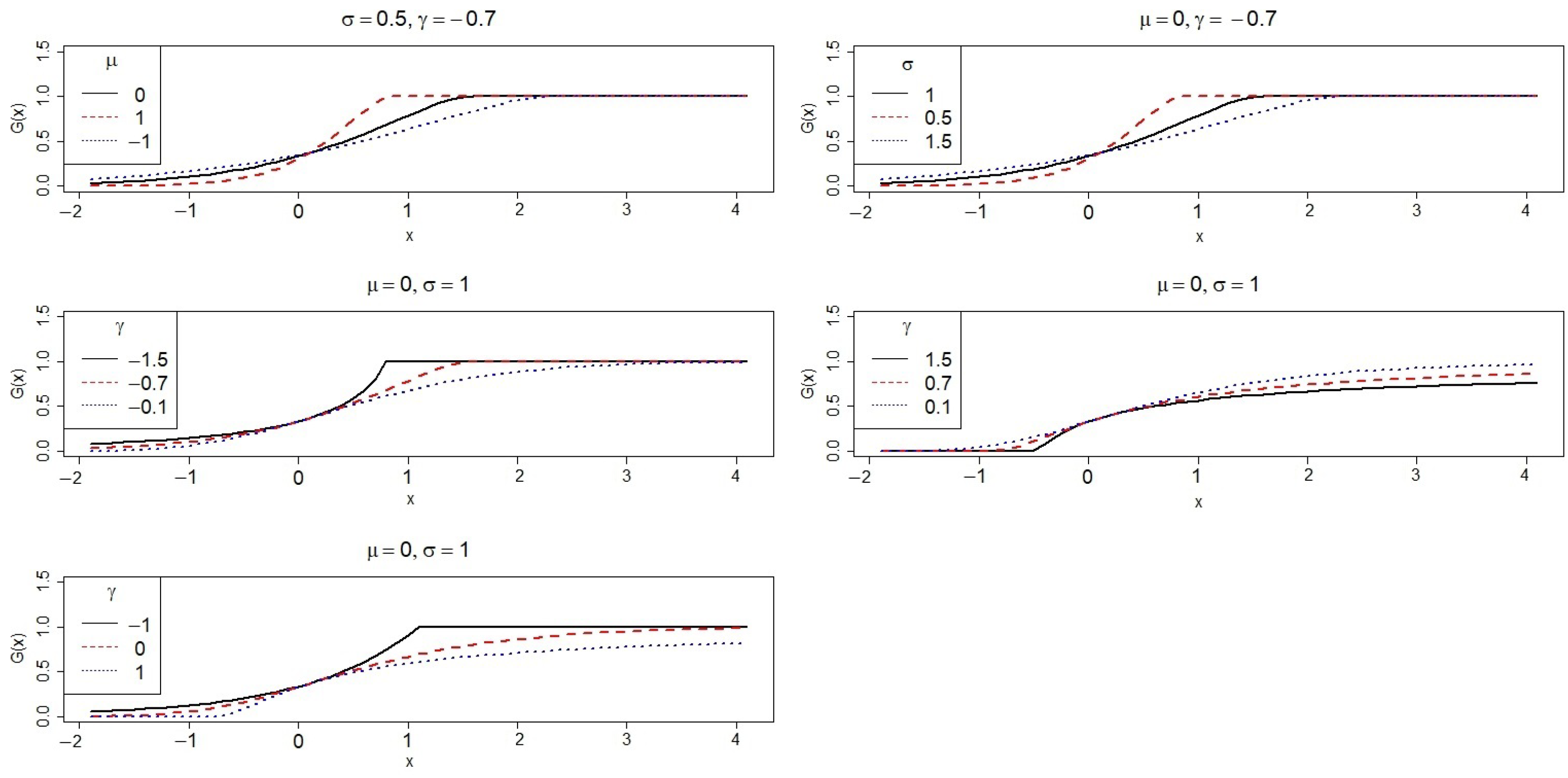
The paper is organized as follows: In Section 2, all the general results needed to carry out the studies are presented. Thus, in this section, the cumulative distribution functions (CDFs) and PDFs of the Gumbel–Hougaard, Frank, and Clayton copulas are presented. Additionally, the PDF and some properties of the GEV distribution are also presented, as well as the estimation guidelines for R. Section 3 presents a simulation study. The performance of the maximum likelihood estimator of R is evaluated and compared with a nonparametric estimator. In Section 4, we deal with three real situations involving asset selection via comparison of log-returns, assessment of credit risk based on income and consumption data, and the comparison of minimum monthly flow rates. Then, Section 5 presents the conclusions.

2. Preliminaries

In this section, we present definitions and results which will be used subsequently.

2.1. Some Bivariate Copulas

The CDF of the Gumbel–Hougaard copula is given by [23]

$$C^{GH}(u,v;\theta )=exp\left\{-{\left[{(-logu)}^{\frac{1}{\theta }}+{(-logv)}^{\frac{1}{\theta }}\right]}^{\theta }\right\},\theta \in (0,1],$$

(2)

where u and v are the marginal distribution functions of random variables X and Y, respectively. Observe that if $\theta =1$, then $C^{GH}(u,v;1)=uv$, that is, X and Y are independent.

The CDFs of the Frank copula and the Clayton copula are given, respectively, by [23]

$$C^F(u,v;\theta )=-\frac{1}{\theta }log\left(1+\frac{(exp\{-\theta u\}-1)(exp\{-\theta v\}-1)}{exp\{-\theta \}-1}\right),\theta \in \mathbb{R}-\left\{0\right\},$$

(3)

and

$$C^C(u,v;\theta )=max{\left\{\left(u^{-\theta }+v^{-\theta }-1\right);0\right\}}^{-\frac{1}{\theta }},\theta \in [-1,\infty )-\left\{0\right\}.$$

(4)

In order to obtain the PDF associated with each CDF, it suffices to consider that

$$c(u,v;\theta )=\frac{{\partial }^{2}C(u,v;\theta )}{\partial u\partial v}.$$

Thus,

Table 1. Copulas, PDFs, and their parameter space.

Copula	$\mathit{c}(\mathit{u},\mathit{v};\mathit{\theta })$	Parameter Space
Gumbel–Hougaard	$\frac{C(u,v;\theta ){(logu logv)}^{\frac{1}{\theta }-1}}{uv{\left[{(-logu)}^{\frac{1}{\theta }}+{(-logv)}^{\frac{1}{\theta }}\right]}^{2-\theta }}\left\{{\left[{(-logu)}^{\frac{1}{\theta }}+{(-logv)}^{\frac{1}{\theta }}\right]}^{\theta }+\frac{1}{\theta }-1\right\}$	$\theta \in (0,1]$
Frank	$\frac{-\theta exp\{-\theta (u+v\left)\right\}(exp\{-\theta \}-1)}{{(exp\{-\theta \}-exp\{-\theta u\}-exp\{-\theta v\}+exp\{-\theta (u+v)\})}^2}$	$\theta \in \mathbb{R}-\left\{0\right\}$
Clayton	$(1+\theta ){\left(uv\right)}^{(-1-\theta )}{(-1+u^{-\theta }+v^{-\theta })}^{-2-1/\theta }$	$\theta \in (0,\infty )$

presents the PDFs of the Gumbel–Hougaard, Frank, and Clayton copulas.

It can be seen in Table 1 that by restricting the parameter space of the Clayton copulas from $\theta \in [-1,\infty )-\left\{0\right\}$ to $\theta \in (0,\infty )$, the $\max \left\{\right\}$ operator can be disregarded.

Estimation of the Copula Parameter

The estimation of $\theta$ can be performed by means of an MLE (maximum likelihood estimator). In this case, given a random sample $(x_i,y_i)$, $i=1,\dots ,n$, the MLE of $\widehat{\theta }$ is given by

$$\widehat{\theta }=arg\underset{\theta }{max}\sum _{i=1}^{n}logc(F\left(x_i\right),G\left(y_i\right);\theta ).$$

(5)

2.2. GEV Distribution

Let X be a random variable with GEV distribution, denoted by X∼$GEV(\mu ,\sigma ,\gamma )$, where $\mu \in \mathbb{R}$ is the location parameter, $\sigma \in {\mathbb{R}}_{+}$ is the scale parameter, and $\gamma \in \mathbb{R}$ is the shape parameter. Its CDF is given by

$$G(x;\mu ,\sigma ,\gamma )=exp\left\{-{\left[1+\frac{\gamma }{\sigma }\left(x-\mu \right)\right]}^{-\frac{1}{\gamma }}\right\},1+\frac{\gamma }{\sigma }(x-\mu )>0.$$

(6)

The support of G depends on the sign of shape $\gamma$ as follows:

$$suppG=\left\{\begin{array}{cc}(\mu -\sigma /\gamma ,\infty ),& \gamma >0,\\ (-\infty ,\mu -\sigma /\gamma ),& \gamma <0,\\ \mathbb{R},& \gamma =0.\end{array}\right.$$

Then, the corresponding PDF is given by

$$g(x;\mu ,\sigma ,\gamma )=G(x,\gamma ,\mu ,\sigma )\frac{1}{\sigma }{\left[1+\frac{\gamma }{\sigma }\left(x-\mu \right)\right]}^{-\frac{1}{\gamma }-1},1+\frac{\gamma }{\sigma }(x-\mu )>0.$$

(7)

Figure 1 and Figure 2 show the behaviour of g and G for some parameter choices. Note that the location parameter shifts the curve, the scale controls dispersion, and the density changes according to the sign of the shape.

Estimation of GEV RV Parameters

Consider an observed random sample $\mathbf{x}=(x_1,x_2,\dots ,x_n)$ of a GEV-distributed RV. The likelihood function is given by

$$L(\mu ,\sigma ,\gamma ;\mathbf{x})=\prod _{i=1}^{n}g(x_i;\mu ,\sigma ,\gamma ){\mathbb{1}}_{1+\gamma (x_i-\mu )/\sigma >0},$$

(8)

where ${\mathbb{1}}_A$ denotes the indicator function of set A. Note that the support of G depends on the parameter choice (except for the case where $\gamma =0$). Thus, usual regularity conditions are not satisfied. Nevertheless, it is possible to perform maximum likelihood estimation, which formally is written as

$$(\widehat{\mu },\widehat{\sigma },\widehat{\gamma })=arg\underset{\mu ,\sigma ,\gamma }{max}L(\mu ,\sigma ,\gamma ;\mathbf{x}).$$

(9)

Observe that for $\gamma =0$, we can use the gradient vector of the likelihood function to find the estimator. For the case where $\gamma \ne 0$, that approach does not work, so numerical methods are required. For a detailed reading of the subject, we refer the reader to [7].

2.3. Estimation of Stress–Strength Probability

Let X and Y be RVs with joint PDF

$$f_{X,Y}(x,y)=c(F\left(x\right),G\left(y\right);\theta )f\left(x\right)g\left(x\right),$$

where the marginal PDFs are $f\left(x\right)=F^{\prime }\left(x\right)$ and $g\left(y\right)=G^{\prime }\left(y\right)$, respectively, and $\theta$ is the association parameter. We can write the stress–strength reliability probability as [23,24]

$$R=P(X<Y)={\int }_{-\infty }^{\infty }{\int }_{-\infty }^{y}c\left(F\left(x\right),G\left(y\right);\theta \right)f\left(x\right)g\left(y\right)dxdy={\int }_0^1{\int }_0^{F\left(G^{-1}\left(v\right)\right)}c(u,v;\theta )dudv.$$

(10)

Assuming that X∼$GEV({\mu }_x,{\sigma }_x,{\gamma }_x)$ and Y∼$GEV({\mu }_y,{\sigma }_y,{\gamma }_y)$, we have

$$R=R({\mu }_x,{\sigma }_x,{\gamma }_x,{\mu }_y,{\sigma }_y,{\gamma }_y,\theta ).$$

Since R is an integral function (measurable), we can estimate R using the invariance property of likelihood estimators through estimates $({\widehat{\mu }}_x,{\widehat{\sigma }}_x,{\widehat{\gamma }}_x,{\widehat{\mu }}_y,{\widehat{\sigma }}_y,{\widehat{\gamma }}_y,\widehat{\theta })$, that is,

$$\widehat{R}=R({\widehat{\mu }}_x,{\widehat{\sigma }}_x,{\widehat{\gamma }}_x,{\widehat{\mu }}_y,{\widehat{\sigma }}_y,{\widehat{\gamma }}_y,\widehat{\theta }).$$

(11)

As indicated, we will consider the method of inference functions for margins [29], where the parameters of the marginal distributions are estimated separately from the parameters of the copula. One may observe that (10) and (11) depend on integrals of the copula density function. In such cases, numerical integration algorithms can be readily used to properly evaluate the integrals involved. In the present paper, a Monte Carlo integration approach is considered. This way, firstly, we generate uniform random points $v_1,\dots v_k$ on $[0,1]$; then, uniform random points $u_j$ are generated on $[0,F\left(G^{-1}\left(v_j\right)\right)]$, for each $j=1,\dots ,k$. Finally, we estimate $\widehat{R}$ as

$$\widehat{R}\approx \frac{1}{k}\sum _{j=1}^{k}c(u_j,v_j;\widehat{\theta })\times [1-0]\times [F(G^{-1}(v_j;{\widehat{\mu }}_y,{\widehat{\sigma }}_y,{\widehat{\gamma }}_y);{\widehat{\mu }}_x,{\widehat{\sigma }}_x,{\widehat{\gamma }}_x)-0].$$

In the next sections, we will compare the results of $\widehat{R}$ with a nonparametric estimator denoted by ${\widehat{R}}_{NP}$, which is defined as

$${\widehat{R}}_{NP}=\frac{1}{n}\sum _{j=1}^n{\mathbb{1}}_{\{x_j\le y_j\}},$$

where ${\mathbb{1}}_A$ denotes the indicator function on set A and n is the sample size.

Algorithm 1 describes the approach used in Section 4 to obtain bootstrap confidence intervals of the estimates of R.    

Algorithm 1: Let $(\mathit{x},\mathit{y})$ be a sample of size $\mathit{n}$ and $\mathit{M}$ be a positive integer denoting the number of bootstrap repetitions.

Step 1 Generate bootstrap samples ${(\mathit{x},\mathit{y})}_{\mathbf{0}}$.

Step 2 Compute the estimates $({\widehat{\mathit{\mu }}}_{\mathit{x}},{\widehat{\mathit{\sigma }}}_{\mathit{x}},{\widehat{\mathit{\gamma }}}_{\mathit{x}},{\widehat{\mathit{\mu }}}_{\mathit{y}},{\widehat{\mathit{\sigma }}}_{\mathit{y}},{\widehat{\mathit{\gamma }}}_{\mathit{y}},\widehat{\mathit{\theta }})$ based on ${(\mathit{x},\mathit{y})}_{\mathbf{0}}$. In this case, the parameters of each distribution are individually estimated by using (9), and then the corresponding uniform-transformed vectors are considered in (5) to estimate $\widehat{\mathit{\theta }}$.

Step 3 Obtain ${\widehat{\mathit{R}}}_{\mathbf{0}}=\widehat{\mathit{R}}({\widehat{\mathit{\mu }}}_{\mathit{x}},{\widehat{\mathit{\sigma }}}_{\mathit{x}},{\widehat{\mathit{\gamma }}}_{\mathit{x}},{\widehat{\mathit{\mu }}}_{\mathit{y}},{\widehat{\mathit{\sigma }}}_{\mathit{y}},{\widehat{\mathit{\gamma }}}_{\mathit{y}},\widehat{\mathit{\theta }})$.

Step 4 Repeat steps $\mathbf{1}$ to $\mathbf{3}$$\mathit{M}$ times.

Step 5 The approximate $\mathbf{100}(\mathbf{1}-\mathit{\alpha })\%$ confidence interval of $\widehat{\mathit{R}}$ is given by $[{\widehat{\mathit{R}}}_{\mathit{M}}(\mathit{\alpha }/\mathbf{2}),{\widehat{\mathit{R}}}_{\mathit{M}}(\mathbf{1}-\mathit{\alpha }/\mathbf{2})]$, where ${\widehat{\mathit{R}}}_{\mathit{M}}\left(\mathit{\alpha }\right)\approx {\widehat{\mathit{G}}}^{-\mathbf{1}}\left(\mathit{\alpha }\right)$ and $\widehat{\mathit{G}}$ is the cumulative distribution function of $\widehat{\mathit{R}}$.

3. Simulation Results

To evaluate the performance of estimates $\widehat{R}$ and ${\widehat{R}}_{NP}$, we simulate random samples from the copulas given in (2), (3), and (4) with GEV marginals. The random samples are simulated using the conditional distributions of random vectors $\mathbf{U}=\{U_1,U_2\}$. In the bivariate case, we shall follow the steps described below [30], given a copula C:

• Obtain a sample $u_2$ from $U_2\sim U[0,1]$, i.e., uniform on [0,1].
• Compute the function (partial derivatives of each copula are presented in Appendix A) $F_{u_1|u_2}\left(u_1\right):=\frac{\partial }{\partial u_2}C(u_1,u_2){|}_{U_2=u_2},u_1\in [0,1]$. This function is nothing but $\mathrm{P}(U_1\le u_1|U_2=u_2)$.
• Compute the generalized inverse $F_{u_1|u_2}^{-1}\left(v\right):=inf\{u_1>0;F_{u_1|u_2}\left(u_1\right)\ge v\},v\in (0,1).$
• Obtain a sample v from $V\sim U[0,1]$, independent of $U_2$.
• Define $u:=F_{u_1|u_2}^{-1}\left(v\right)$, and take $(u,u_2)$ as the random vector of copula C.

Steps 1–5 described above give us a random vector with uniform marginal distributions (cf. [31]). We can generate a random vector with distribution C and marginals $GEV({\mu }_x,{\sigma }_x,{\gamma }_x)$ and $GEV({\mu }_y,{\sigma }_y,{\gamma }_y)$ as

$$(G^{-1}(u;{\mu }_x,{\sigma }_x,{\gamma }_x),G^{-1}(u_2;{\mu }_y,{\sigma }_y,{\gamma }_y)).$$

where $G(.)$ denotes the CDF of GEV RVs.

The values of ${\mu }_x,{\sigma }_x,{\gamma }_x,{\mu }_y,{\sigma }_y,{\gamma }_y,$ and $\theta$ and the sample size (n) are pre-specified. Monte Carlo simulations were implemented in R [32] with $M=100$ replications. To compare the estimates, we take the mean ${\widehat{R}}_{MC}$ of the 100 bootstrap samples, the bias, and the root mean squared error (RMSE) when compared with the true R.

The only R package utilized in our study was extRemes to use the pdf and cdf of the GEV marginal distribution, in addition to the fevd function. Following the adjustment of the marginals, we estimated the dependence parameter ($\theta$) using Equation (5). All other algorithms employed in this study were programmed based on the procedures outlined in this work. In order to enable readers to apply the methodology hereby proposed, the codes are available at a public repository [33].

In

Table 2. Monte Carlo simulation for Gumbel–Hougaard copula with GEV marginals and $n=100$.

${\mathit{\mu }}_1$	${\mathit{\sigma }}_1$	${\mathit{\gamma }}_1$	${\mathit{\mu }}_2$	${\mathit{\sigma }}_2$	${\mathit{\gamma }}_2$	$\mathit{\theta }$	R	${\widehat{\mathit{R}}}_{\mathit{MC}}$	Bias	RMSE	${\widehat{\mathit{R}}}_{\mathit{NP}}$	${\mathit{Bias}}_{\mathit{NP}}$	${\mathit{RMSE}}_{\mathit{NP}}$
0.0	0.7	−0.3	0.0	1.0	−1.0	0.3	0.3600	0.4047	0.0447	0.0692	0.3679	0.0079	0.0470
0.0	0.9	−0.3	0.0	1.5	−1.0	0.3	0.4306	0.4261	−0.0045	0.1393	0.4362	0.0056	0.0422
0.0	0.7	−1.0	0.0	1.0	−1.0	0.3	0.6361	0.6194	−0.0166	0.0719	0.6511	0.0150	0.0528
0.0	0.9	−1.0	0.0	1.5	−1.0	0.3	0.6431	0.5814	−0.0617	0.1616	0.6571	0.0140	0.0454
0.0	0.5	−1.5	0.0	1.5	−1.5	0.3	0.6587	0.6149	−0.0439	0.0874	0.6621	0.0034	0.0474
0.0	0.7	−1.5	0.0	1.0	−1.5	0.3	0.6596	0.5925	−0.0672	0.1306	0.6723	0.0127	0.0498
0.0	0.9	−1.5	0.0	1.5	−1.5	0.3	0.6649	0.6099	−0.0549	0.1118	0.6739	0.0090	0.0490
0.0	0.7	−0.3	0.0	1.0	−1.0	0.5	0.4030	0.4207	0.0178	0.0576	0.3953	−0.0077	0.0496
0.0	0.9	−0.3	0.0	1.5	−1.0	0.5	0.4450	0.4182	−0.0268	0.1303	0.4361	−0.0089	0.0578
0.0	0.7	−1.0	0.0	1.0	−1.0	0.5	0.6107	0.5984	−0.0123	0.0785	0.6314	0.0207	0.0551
0.0	0.9	−1.0	0.0	1.5	−1.0	0.5	0.6202	0.5666	−0.0537	0.1595	0.6386	0.0184	0.0511
0.0	0.5	−1.5	0.0	1.5	−1.5	0.5	0.6563	0.6135	−0.0428	0.1119	0.6588	0.0025	0.0414
0.0	0.7	−1.5	0.0	1.0	−1.5	0.5	0.6434	0.6013	−0.0421	0.0949	0.6486	0.0052	0.0490
0.0	0.9	−1.5	0.0	1.5	−1.5	0.5	0.6448	0.6062	−0.0386	0.0978	0.6567	0.0119	0.0453
0.0	0.7	−0.3	0.0	1.0	−1.0	0.7	0.4287	0.4492	0.0204	0.0463	0.4316	0.0029	0.0510
0.0	0.9	−0.3	0.0	1.5	−1.0	0.7	0.4647	0.4229	−0.0417	0.1646	0.4654	0.0007	0.0530
0.0	0.7	−1.0	0.0	1.0	−1.0	0.7	0.5896	0.5652	−0.0244	0.0921	0.5892	−0.0004	0.0545
0.0	0.9	−1.0	0.0	1.5	−1.0	0.7	0.6011	0.5448	−0.0563	0.1655	0.6129	0.0118	0.0498
0.0	0.5	−1.5	0.0	1.5	−1.5	0.7	0.6456	0.6072	−0.0384	0.1314	0.6568	0.0112	0.0467
0.0	0.7	−1.5	0.0	1.0	−1.5	0.7	0.6186	0.5836	−0.0350	0.1159	0.6244	0.0058	0.0472
0.0	0.9	−1.5	0.0	1.5	−1.5	0.7	0.6217	0.5930	−0.0287	0.0905	0.6255	0.0038	0.0410
0.0	0.7	−0.3	0.0	1.0	−1.0	0.9	0.4542	0.4577	0.0036	0.0575	0.4529	−0.0013	0.0515
0.0	0.9	−0.3	0.0	1.5	−1.0	0.9	0.4858	0.4275	−0.0583	0.1587	0.4819	−0.0039	0.0485
0.0	0.7	−1.0	0.0	1.0	−1.0	0.9	0.5701	0.5676	−0.0025	0.0703	0.5731	0.0030	0.0470
0.0	0.9	−1.0	0.0	1.5	−1.0	0.9	0.5851	0.5332	−0.0519	0.1605	0.5934	0.0083	0.0525
0.0	0.5	−1.5	0.0	1.5	−1.5	0.9	0.6336	0.5908	−0.0428	0.1371	0.6374	0.0038	0.0531
0.0	0.7	−1.5	0.0	1.0	−1.5	0.9	0.5965	0.5809	−0.0156	0.0938	0.6054	0.0089	0.0474
0.0	0.9	−1.5	0.0	1.5	−1.5	0.9	0.6028	0.5805	−0.0224	0.1436	0.6223	0.0195	0.0520

,

Table 3. Monte Carlo simulation for Frank copula with GEV marginals and $n=100$.

${\mathit{\mu }}_1$	${\mathit{\sigma }}_1$	${\mathit{\gamma }}_1$	${\mathit{\mu }}_2$	${\mathit{\sigma }}_2$	${\mathit{\gamma }}_2$	$\mathit{\theta }$	R	${\widehat{\mathit{R}}}_{\mathit{MC}}$	Bias	RMSE	${\widehat{\mathit{R}}}_{\mathit{NP}}$	${\mathit{Bias}}_{\mathit{NP}}$	${\mathit{RMSE}}_{\mathit{NP}}$
1.0	0.7	−0.3	1.0	1.0	−1.0	−5.0	0.4960	0.5029	0.0069	0.0643	0.5041	0.0081	0.0579
1.0	0.9	−0.3	1.0	1.5	−1.0	−5.0	0.5259	0.4598	−0.0661	0.1574	0.5269	0.0010	0.0486
1.0	0.7	−1.0	1.0	1.0	−1.0	−5.0	0.5284	0.5288	0.0004	0.0530	0.5280	−0.0004	0.0532
1.0	0.9	−1.0	1.0	1.5	−1.0	−5.0	0.5458	0.4819	−0.0639	0.1721	0.5467	0.0009	0.0492
1.0	0.5	−1.5	1.0	1.5	−1.5	−5.0	0.5976	0.5562	−0.0415	0.1462	0.6017	0.0041	0.0573
1.0	0.7	−1.5	1.0	1.0	−1.5	−5.0	0.5493	0.5159	−0.0334	0.1199	0.5425	−0.0068	0.0492
1.0	0.9	−1.5	1.0	1.5	−1.5	−5.0	0.5628	0.5517	−0.0111	0.1386	0.5641	0.0013	0.0495
1.0	0.7	−0.3	1.0	1.0	−1.0	−0.9	0.4740	0.4688	−0.0052	0.0587	0.4729	−0.0011	0.0546
1.0	0.9	−0.3	1.0	1.5	−1.0	−0.9	0.5038	0.4440	−0.0598	0.1535	0.4897	−0.0141	0.0553
1.0	0.7	−1.0	1.0	1.0	−1.0	−0.9	0.5525	0.5575	0.0050	0.0608	0.5605	0.0080	0.0522
1.0	0.9	−1.0	1.0	1.5	−1.0	−0.9	0.5698	0.5059	−0.0640	0.1782	0.5734	0.0036	0.0537
1.0	0.5	−1.5	1.0	1.5	−1.5	−0.9	0.6211	0.5846	−0.0366	0.1337	0.6281	0.0070	0.0515
1.0	0.7	−1.5	1.0	1.0	−1.5	−0.9	0.5771	0.5534	−0.0237	0.1135	0.5721	−0.0050	0.0576
1.0	0.9	−1.5	1.0	1.5	−1.5	−0.9	0.5866	0.5498	−0.0368	0.1328	0.5864	−0.0002	0.0480
1.0	0.7	−0.3	1.0	1.0	−1.0	0.9	0.4569	0.4509	−0.0060	0.0580	0.4495	−0.0074	0.0493
1.0	0.9	−0.3	1.0	1.5	−1.0	0.9	0.4883	0.4260	−0.0623	0.1598	0.4774	−0.0109	0.0529
1.0	0.7	−1.0	1.0	1.0	−1.0	0.9	0.5690	0.5775	0.0085	0.0629	0.5711	0.0021	0.0512
1.0	0.9	−1.0	1.0	1.5	−1.0	0.9	0.5863	0.5207	−0.0656	0.1805	0.5876	0.0013	0.0463
1.0	0.5	−1.5	1.0	1.5	−1.5	0.9	0.6345	0.6002	−0.0343	0.1103	0.6277	−0.0068	0.0475
1.0	0.7	−1.5	1.0	1.0	−1.5	0.9	0.5966	0.5579	−0.0387	0.1443	0.6015	0.0049	0.0559
1.0	0.9	−1.5	1.0	1.5	−1.5	0.9	0.6036	0.5597	−0.0439	0.1574	0.6035	−0.0001	0.0522
1.0	0.7	−0.3	1.0	1.0	−1.0	5.0	0.4166	0.4119	−0.0047	0.0542	0.4117	−0.0049	0.0506
1.0	0.9	−0.3	1.0	1.5	−1.0	5.0	0.4537	0.4006	−0.0530	0.1665	0.4530	−0.0007	0.0500
1.0	0.7	−1.0	1.0	1.0	−1.0	5.0	0.6046	0.6087	0.0041	0.0715	0.6041	−0.0005	0.0488
1.0	0.9	−1.0	1.0	1.5	−1.0	5.0	0.6278	0.5706	−0.0572	0.1869	0.6300	0.0022	0.0504
1.0	0.5	−1.5	1.0	1.5	−1.5	5.0	0.6550	0.6224	−0.0326	0.1229	0.6584	0.0034	0.0499
1.0	0.7	−1.5	1.0	1.0	−1.5	5.0	0.6388	0.5944	−0.0445	0.1267	0.6333	−0.0055	0.0485
1.0	0.9	−1.5	1.0	1.5	−1.5	5.0	0.6430	0.6180	−0.0250	0.1399	0.6495	0.0065	0.0497

and

Table 4. Monte Carlo simulations for Clayton copula with GEV marginals and $n=100$.

${\mathit{\mu }}_1$	${\mathit{\sigma }}_1$	${\mathit{\gamma }}_1$	${\mathit{\mu }}_2$	${\mathit{\sigma }}_2$	${\mathit{\gamma }}_2$	$\mathit{\theta }$	R	${\widehat{\mathit{R}}}_{\mathit{MC}}$	Bias	RMSE	${\widehat{\mathit{R}}}_{\mathit{NP}}$	${\mathit{Bias}}_{\mathit{NP}}$	${\mathit{RMSE}}_{\mathit{NP}}$
0.0	0.7	−0.3	0.0	1.0	−1.0	1.5	0.4048	0.4014	−0.0034	0.0462	0.4000	−0.0048	0.0512
0.0	0.9	−0.3	0.0	1.5	−1.0	1.5	0.4434	0.4152	−0.0282	0.1164	0.4405	−0.0029	0.0447
0.0	0.7	−1.0	0.0	1.0	−1.0	1.5	0.5662	0.5800	0.0138	0.0609	0.5641	−0.0021	0.0453
0.0	0.9	−1.0	0.0	1.5	−1.0	1.5	0.5836	0.5271	−0.0565	0.1881	0.5973	0.0137	0.0521
0.0	0.5	−1.5	0.0	1.5	−1.5	1.5	0.6265	0.5876	−0.0389	0.1395	0.6321	0.0056	0.0465
0.0	0.7	−1.5	0.0	1.0	−1.5	1.5	0.6029	0.5729	−0.0301	0.1322	0.6084	0.0055	0.0525
0.0	0.9	−1.5	0.0	1.5	−1.5	1.5	0.6125	0.5716	−0.0409	0.1332	0.6068	−0.0057	0.0482
0.0	0.7	−0.3	0.0	1.0	−1.0	2.5	0.3794	0.3747	−0.0048	0.0575	0.3754	−0.0040	0.0438
0.0	0.9	−0.3	0.0	1.5	−1.0	2.5	0.4244	0.3782	−0.0462	0.1665	0.4301	0.0057	0.0519
0.0	0.7	−1.0	0.0	1.0	−1.0	2.5	0.5642	0.5892	0.0250	0.0768	0.5682	0.0040	0.0489
0.0	0.9	−1.0	0.0	1.5	−1.0	2.5	0.5832	0.5486	−0.0346	0.1673	0.5933	0.0101	0.0409
0.0	0.5	−1.5	0.0	1.5	−1.5	2.5	0.6234	0.5658	−0.0576	0.1758	0.6281	0.0047	0.0493
0.0	0.7	−1.5	0.0	1.0	−1.5	2.5	0.6042	0.5658	−0.0384	0.1222	0.6004	−0.0038	0.0463
0.0	0.9	−1.5	0.0	1.5	−1.5	2.5	0.6076	0.5885	−0.0191	0.1359	0.6230	0.0154	0.0512
0.0	0.7	−0.3	0.0	1.0	−1.0	2.8	0.3734	0.3695	−0.0039	0.0574	0.3700	−0.0034	0.0444
0.0	0.9	−0.3	0.0	1.5	−1.0	2.8	0.4214	0.3682	−0.0531	0.1485	0.4079	−0.0135	0.0504
0.0	0.7	−1.0	0.0	1.0	−1.0	2.8	0.5639	0.5838	0.0199	0.1003	0.5747	0.0108	0.0484
0.0	0.9	−1.0	0.0	1.5	−1.0	2.8	0.5835	0.5418	−0.0416	0.1724	0.5839	0.0004	0.0503
0.0	0.5	−1.5	0.0	1.5	−1.5	2.8	0.6228	0.5723	−0.0505	0.1544	0.6174	−0.0054	0.0437
0.0	0.7	−1.5	0.0	1.0	−1.5	2.8	0.6046	0.5488	−0.0558	0.1691	0.5975	−0.0071	0.0539
0.0	0.9	−1.5	0.0	1.5	−1.5	2.8	0.6077	0.5685	−0.0392	0.1564	0.6056	−0.0021	0.0583
0.0	0.7	−0.3	0.0	1.0	−1.0	3.0	0.3697	0.3664	−0.0033	0.0574	0.3653	−0.0044	0.0443
0.0	0.9	−0.3	0.0	1.5	−1.0	3.0	0.4197	0.3980	−0.0217	0.1506	0.4130	−0.0067	0.0487
0.0	0.7	−1.0	0.0	1.0	−1.0	3.0	0.5637	0.5983	0.0346	0.0835	0.5782	0.0145	0.0538
0.0	0.9	−1.0	0.0	1.5	−1.0	3.0	0.5838	0.5442	−0.0396	0.1734	0.5896	0.0058	0.0514
0.0	0.5	−1.5	0.0	1.5	−1.5	3.0	0.6225	0.5798	−0.0427	0.1566	0.6219	−0.0006	0.0484
0.0	0.7	−1.5	0.0	1.0	−1.5	3.0	0.6049	0.5769	−0.0281	0.0969	0.6046	−0.0003	0.0464
0.0	0.9	−1.5	0.0	1.5	−1.5	3.0	0.6079	0.5788	−0.0291	0.1174	0.6092	0.0013	0.0438

, we present the performance of estimators ${\widehat{R}}_{MC}$ and ${\widehat{R}}_{NP}$ for Gumbel–Hougard, Frank, and Clayton copulas with GEV marginals, respectively. Overall, estimators ${\widehat{R}}_{NP}$ seem to be better than ${\widehat{R}}_{MC}$, presenting lower bias and RMSE.

4. Real Data Set Applications

We discuss three applications using real data. We study the validity of the model for all the cases and show that the Gumbel–Hougaard, Frank, or Clayton copula with GEV marginals adequately fit the data sets considered. For all the analyses carried out, the normal QQ plots are presented to assess the tail behaviour of the data sets compared with the best-fitted normal random variable.

4.1. Asset Selection

Using metrics of type $P(X<Y)$ can serve as a guide for selecting financial assets when managing a portfolio. Rather than relying on the traditional method of comparing the expected values of X and Y (according to modern portfolio theory), we explore the use of a reliability measure, $P(X<Y)$, as an alternative parameter for evaluating returns.

We compare the stock price log-returns from tickers (traded on BOVESPA, São Paulo Stock Exchange) BBAS3.SA, ITUB4.SA, UGPA3.SA, PETR3.SA, VALE3.SA, VIIA3.SA, and MGLU3.SA. These stocks are from companies representing a wide variety of economic sectors, namely, banking (BBAS3 and ITUB4), gas and oil extraction and commercialization (UGPA3 and PETR3), mining (VALE3), and retail (VIIA3 and MGLU3). From now on, we will omit the “.SA” suffix present on the tickers under analysis. The daily closing prices between 1 January 2022 and 30 April 2023 were retrieved from Yahoo! Finance. Summary statistics for the data sets are presented in

Table 5. Summary statistics for stock price log-returns ($n=331$).

Data Set	Min.	1st Qu	Median	Mean	3rd Qu.	Max.	Std. dv.	Skewness	Kurtosis
BBAS3	−0.1057	−0.0097	0.0019	0.0012	0.0136	0.0736	0.0204	−0.3452	5.7413
ITUB4	−0.0492	−0.0105	0.0004	0.0006	0.0109	0.0794	0.0172	0.3809	4.4864
UGPA3	−0.0802	−0.0169	−0.0023	0.0001	0.0158	0.0771	0.0252	0.0306	3.0732
PETR3	−0.1270	−0.0136	0.0007	−0.0005	0.0159	0.0849	0.0280	−1.0420	6.3563
VALE3	−0.0689	−0.0140	0.0001	−0.0002	0.0128	0.0989	0.0231	0.4092	4.5967
VIIA3	−0.1075	−0.0344	−0.0059	−0.0030	0.0231	0.1504	0.0447	0.6144	3.6044
MGLU3	−0.1435	−0.0329	−0.0043	−0.0021	0.0284	0.1635	0.0502	0.1849	3.1167

. Figure 3 presents the boxplots from the log-returns, showing certain symmetry of log-returns around zero and greater variability for MGLU3 and VIIA3. The dependence structure between the log-returns of the data sets is shown in Figure 4, and it is measured with correlation matrices in

Table 6. Pearson correlation matrix.

	BBAS3	ITUB4	UGPA3	PETR3	VALE3	VIIA3	MGLU3
BBAS3	1.00	0.56	0.17	0.07	−0.36	−0.32	−0.24
ITUB4	0.56	1.00	0.24	0.39	−0.14	0.25	0.24
UGPA3	0.17	0.24	1.00	0.30	0.18	0.38	0.54
PETR3	0.07	0.39	0.30	1.00	−0.22	0.70	0.53
VALE3	−0.36	−0.14	0.18	−0.22	1.00	0.12	0.35
VIIA3	−0.32	0.25	0.38	0.70	0.12	1.00	0.87
MGLU3	−0.24	0.24	0.54	0.53	0.35	0.87	1.00

,

Table 7. Spearman rank correlation matrix.

	BBAS3	ITUB4	UGPA3	PETR3	VALE3	VIIA3	MGLU3
BBAS3	1.00	0.58	0.21	0.06	−0.33	−0.26	−0.07
ITUB4	0.58	1.00	0.33	0.37	−0.06	0.32	0.38
UGPA3	0.21	0.33	1.00	0.30	0.14	0.31	0.48
PETR3	0.06	0.37	0.30	1.00	−0.23	0.74	0.55
VALE3	−0.33	−0.06	0.14	−0.23	1.00	0.09	0.25
VIIA3	−0.26	0.32	0.31	0.74	0.09	1.00	0.81
MGLU3	−0.07	0.38	0.48	0.55	0.25	0.81	1.00

and

Table 8. Kendall rank correlation matrix.

	BBAS3	ITUB4	UGPA3	PETR3	VALE3	VIIA3	MGLU3
BBAS3	1.00	0.40	0.16	0.05	−0.22	−0.17	−0.02
ITUB4	0.40	1.00	0.22	0.25	0.01	0.22	0.27
UGPA3	0.16	0.22	1.00	0.20	0.09	0.22	0.34
PETR3	0.05	0.25	0.20	1.00	−0.15	0.51	0.36
VALE3	−0.22	0.01	0.09	−0.15	1.00	0.06	0.16
VIIA3	−0.17	0.22	0.22	0.51	0.06	1.00	0.63
MGLU3	−0.02	0.27	0.34	0.36	0.16	0.63	1.00

, which present Pearson, Spearman, and Kendal correlation matrices, respectively. It is now of interest to choose the best copula fit among Gumbel–Hougaard, Frank, and Clayton.

The estimated parameters for the GEV distribution, as well as the p-value of the Kolmogorov–Smirnov (KS) test, are presented in

Table 9. Estimated parameters of GEV distribution and the p-value of the Kolmogorov–Smirnov test.

	$\widehat{\mathit{\mu }}$	$\widehat{\mathit{\sigma }}$	$\widehat{\mathit{\gamma }}$	KS p-Value
BBAS3	−0.01	0.02	−0.25	0.01
ITUB4	−0.01	0.02	−0.15	0.43
UGPA3	−0.01	0.03	−0.26	0.73
PETR3	−0.01	0.03	−0.32	0.00
VALE3	−0.01	0.02	−0.16	0.23
VIIA3	−0.02	0.04	−0.12	0.70
MGLU3	−0.02	0.05	−0.22	0.64

. Figure 5, Figure 6, Figure 7 and Figure 8 show the GEV fits for the data sets. Note that despite the KS test rejecting GEV adjustment for BBAS3 and PETR3 data, a graphical analysis of the histogram and empirical CDF (ECDF) would not necessarily dismiss the suitability of the GEV distribution for those data sets. It is also important to notice that the KS test becomes too sensitive to even small deviations for medium to large sample sizes, which explains this issue.

The log-return pairs $(X,Y)$ selected for comparison were (BBAS3, ITUB4), (UGPA3, MGLU3), (VIIA3, PETR3), (MGLU3, VIIA3), (MGLU3, PETR3) and (VALE3, BBAS3). Deciding the better copula to jointly model the bivariate data was oriented by the AIC (Akaike information criterion), BIC (Bayesian information criterion), and EDC (efficient determination criterion). In

Table 10. Copula dependence estimates and model selection with AIC, BIC, and EDC.

Bivariate Data Set	Copula	$\widehat{\mathit{\theta }}$	AIC	BIC	EDC
(BBAS3, ITUB4)	Gumbel–Hougaard	0.58	−121.74	−54.55	−111.13
	Frank	5.77	−159.13	−91.94	−148.52
	Clayton	0.78	−80.07	−12.88	−69.46
(UGPA3, MGLU3)	Gumbel–Hougaard	0.72	−51.81	15.38	−41.20
	Frank	3.22	−61.22	5.97	−50.61
	Clayton	0.43	−22.73	44.46	−12.12
(VIIA3, PETR3)	Gumbel–Hougaard	0.94	11.24	78.42	21.85
	Frank	0.89	9.08	76.27	19.69
	Clayton	0.05	13.12	80.31	23.73
(MGLU3, VIIA3)	Gumbel–Hougaard	0.43	−301.61	−234.43	−291.00
	Frank	7.98	−297.10	−229.92	−286.50
	Clayton	1.30	−152.77	−85.59	−142.17
(MGLU3, PETR3)	Gumbel–Hougaard	0.93	11.10	78.29	21.71
	Frank	1.03	7.59	74.77	18.19
	Clayton	0.06	12.25	79.44	22.86
(VALE3, BBAS3)	Gumbel–Hougaard	0.95	12.79	79.98	23.40
	Frank	1.08	7.46	74.65	18.07
	Clayton	0.04	12.83	80.02	23.44

, these criteria suggest the Gumbel–Hougaard copula for (MGLU3,VIIA3) and the Frank copula for (BBAS3, ITUB4), (UGPA3, MGLU3), (VIIA3, PETR3), (MGLU3,PETR3), and (VALE3, BBAS3).

In

Table 11. R estimates and 95% confidence intervals.

Bivariate Data Set	$\widehat{\mathit{R}}$	${\widehat{\mathit{R}}}_{\mathit{NP}}$	$95\%\mathit{CI}$
(BBAS3, ITUB4)	$0.4749$	$0.4909$	$(0.4459;0.5224)$
(UGPA3, MGLU3)	$0.4393$	$0.4788$	$(0.4035;0.4949)$
(VIIA3, PETR3)	0.5482	0.5576	$(0.5053;0.5899)$
(MGLU3, VIIA3)	0.4696	0.4667	$(0.4477;0.533)$
(MGLU3, PETR3)	0.5245	0.5455	$(0.4843;0.566)$
(VALE3, BBAS3)	0.5296	0.5242	$(0.4874;0.5689)$

, $CI$ is obtained with the bootstrap approach as in Algorithm 1. In an asset selection scenario, the only conclusive situation is when comparing UGPA3 and MGLU3, since this is the case where $R=1/2$ is not inside the confidence interval $(0.4035;0.4949)$, indicating that UGPA3 returns are greater than MGLU3 in the period analysed. For all the other cases, the analysis is inconclusive.

Figure 9 shows real and simulated data. Figure 10 shows normal QQ plots. We can conclude that the copula models fit the data well. Additionally, it is important to compare different distributions as candidate models for log-returns modelling. We compared the performance of the GEV and normal distributions as models for daily returns, as presented in

Table 12. Model selection for marginals with AIC, BIC, and EDC.

Data Set	Distribution	AIC	BIC	EDC
BBAS3	Normal	1638.59	1657.78	1641.62
	GEV	1613.83	1642.63	1618.38
ITUB4	Normal	1750.27	1769.47	1753.30
	GEV	1747.28	1776.07	1751.82
MGLU3	Normal	1043.51	1062.70	1046.54
	GEV	1046.06	1074.86	1050.61
VIIA3	Normal	1119.85	1139.05	1122.88
	GEV	1141.40	1170.19	1145.94
VALE3	Normal	1556.49	1575.69	1559.52
	GEV	1554.18	1582.97	1558.73
PETR3	Normal	1427.54	1446.74	1430.57
	GEV	1411.09	1439.88	1415.63
UGPA3	Normal	1498.53	1517.73	1501.56
	GEV	1499.31	1528.11	1503.86

. It is possible to see that both GEV and normal distributions provided quite similar modelling capabilities (with the same information criterion values).

4.2. Income–Consumption Data

In order to evaluate R, a public data set of income and consumption data was used. The data (available at https://www.bancaditalia.it/statistiche/tematiche/indagini-famiglie-imprese/bilanci-famiglie/documentazione/ricerca/ricerca.html?min_anno_pubblicazione=2008&max_anno_pubblicazione=2008, accessed on 15 December 2023) come from Bank of Italy’s Survey on Household Income and Wealth from the year 2008.

Income is composed by:

• Payroll income (net wages, salaries, and fringe benefits);
• Pensions and net transfers (pensions, arrears, and other transfers);
• Net self-employment income (self-employment income and entrepreneurial income);
• Property income (either from real estate or from financial assets).

Consumption is composed of the years of durable and non-durable expenditure. Durable expenditure is the balance between bought and sold goods, and non-durable expenditure is composed of monthly expenses (rentals, food, non-food, etc.) and yearly ones.

The same data set was also used in [2]; however, those authors transformed the consumption data, and to the best of our knowledge, we could not obtain the same transformed data following the procedures described in [2]. Therefore, we opted to use the raw data from the survey, available as the data sets RFAM08 (income as Y variable) and RISFAM08 (expenditures as C variable), according to the Survey on Household Income and Wealth 2008 data description file (available at https://www.bancaditalia.it/statistiche/tematiche/indagini-famiglie-imprese/bilanci-famiglie/documentazione/documenti/2008/eng_Legen08.pdf, accessed on 15 December 2023). The filtered sample yielded 7977 households after removing entries whose income or consumption was negative or unavailable.

Table 13. Descriptive statistics for consumption (X) and income (Y).

Data Set	Min.	1st Qu.	Median	Mean	3rd Qu.	Max.	Std. dv.	Skewness
X	1680	15,600	20,760	23,836	28,800	283,100	13,779.52	3.7685
Y	65.7	17,890.5	26,784.2	32,424.4	40,587.0	629,339.7	24,333.25	5.2347

presents descriptive statistics for income (Y) and consumption (which we denote by X). Figure 11 and Figure 12 show data with heavy tails and the fit of the GEV distribution to the density and ECDF of the data. The estimated parameters are presented in

Table 14. Estimated parameters of GEV distribution.

Data Set	$\widehat{\mathit{\mu }}$	$\widehat{\mathit{\sigma }}$	$\widehat{\mathit{\gamma }}$
X	17,753.46	8226.34	0.13
Y	21,993.26	12,807.62	0.20

. The fit of the Frank copula and GEV marginals are also evaluated in Figure 13. Besides, Figure 14 presents the QQ plots of the datasets.

The correlations between consumption and income data are high, evidenced by significant Pearson, Kendall, and Spearman correlation coefficients of 0.7171, 0.6425, and 0.8224, respectively. Despite the GEV distribution effectively modelling the marginals, independence cannot be considered in this context, making the direct application of the results by Quintino et al. [1] unfeasible. Consequently, the preferred approach in this scenario involves modelling dependence using copulas. Referring to

Table 15. Copula dependence estimates and model selection with AIC, BIC, and EDC.

B	$\widehat{\mathit{\theta }}$	AIC	BIC	EDC
Gumbel–Hougaard	0.40	−8410.24	−8298.50	−8393.51
Frank	9.14	−8983.35	−8871.60	−8966.62
Clayton	2.21	−7313.24	−7201.49	−7296.50

, the Frank copula emerges as the optimal choice for jointly modelling variables X and Y, as it demonstrates the most favourable information criterion, compared with the Gumbel–Hougaard and Clayton copulas. Upon estimating R with (10), the resulting value is $\widehat{R}=0.7841$, accompanied by a $95\%$ CI of $(0.7562;0.7957)$. Consequently, this suggests a probability of approximately $79\%$ for a typical family to conclude the year with a positive income balance.

Given that the X and Y data are positive, we can make a comparison between the utilization of the GEV distribution and other familiar distributions, such as Weibull and Gamma, as illustrated in

Table 16. Model selection for marginals with AIC, BIC, and EDC.

Data Set	Model	AIC	BIC	EDC
X	Gamma	170,462.98	170,494.91	170,467.76
	Weibull	171,812.76	171,844.69	171,817.54
	GEV	169,926.30	169,974.19	169,933.47
Y	Gamma	177,934.22	177,966.14	177,939.00
	Weibull	178,862.71	178,894.64	178,867.49
	GEV	169,926.30	169,974.19	169,933.47

.

4.3. Minimum Monthly Flows Of Water

Ramos et al. [34] analysed five real data sets related to minimum monthly flows of water (m³/s) on the Piracicaba River, located in São Paulo state, Brazil. They obtained the data sets from the Department of Water Resources and Power agency manager of water resources of the State of São Paulo from 1960 to 2014.

Considering that Brazil’s electric matrix is mostly composed of hydraulic sources (about 62 % of the total [35]), it is important to understand the monthly changes in the flows of water in order to account for alternative sources of electric generation. Over the months, it may be necessary to use fossil fuel sources to complement the amount of energy generation needed for the whole country. This way, the reliability measures of type $P(X<Y)$ can be used to estimate the amount of fossil fuels that need to be stocked for a given month, comparatively.

Thus,

Table 17. Descriptive statistics for July (X) and September (Y).

Data Set	Min.	1st Qu.	Median	Mean	3rd Qu.	Max.	Std. dv.	Skewness
X	7.26	11.40	13.49	25.41	25.14	174.94	30.97	3.35
Y	6.18	11.12	16.44	28.28	32.91	153.78	29.32	2.45

presents descriptive statistics for the minimum monthly flows of water in September (Y) and July (X). Figure 15 shows the fitted GEV distribution PDFs and CDFs as well as the empirical ones. The QQ plots in Figure 16 indicate good fit quality. Furthermore, the estimated parameters are presented in

Table 18. Estimated parameters of GEV distribution.

Data Set	$\widehat{\mathit{\mu }}$	$\widehat{\mathit{\sigma }}$	$\widehat{\mathit{\gamma }}$
X	12.7542	5.8039	0.7114
Y	13.3178	8.4558	0.7448

.

The correlations among minimum monthly flow data are high, evidenced by significant Pearson, Kendall, and Spearman correlation coefficients of 0.31, 0.15, and 0.21, respectively. Referring to

Table 19. Copula dependence estimates and model selection with AIC, BIC, and EDC.

Copula	$\widehat{\mathit{\theta }}$	AIC	BIC	EDC
Gumbel–Hougaard	0.87	11.87	49.16	16.05
Frank	1.13	12.55	49.84	16.73
Clayton	0.10	13.73	51.02	17.91

, the Gumbel–Hougaard copula emerges as the optimal choice for jointly modelling variables X and Y, as it demonstrates the most favourable information criterion, compared with the Frank and Clayton copulas. Upon estimating R using (10), the resulting value is $\widehat{R}=0.5384$, accompanied by a $95\%$ CI of $(0.3918;0.6899)$. This suggests that the need for contingency in both months is about the same (the minimum flows are statistically equivalent).

As done in previous subsections, by noticing that data sets X and Y are positive, it is possible to perform a comparative analysis of the marginal adjustments of the GEV distribution with those of the Gamma and Weibull models, as illustrated in

Table 20. Model selection for marginals with AIC, BIC, and EDC.

Data Set	Model	AIC	BIC	EDC
X	Gamma	377.69	388.35	378.89
	Weibull	376.39	387.05	377.59
	GEV	342.17	358.15	343.96
Y	Gamma	338.44	349.09	339.63
	Weibull	340.89	351.54	342.08
	GEV	327.42	343.40	329.21

.

5. Conclusions

In reliability assessment, metrics of type $R=P(X<Y)$ are useful, especially when both X and Y need to be statistically compared. The literature has considered cases where both X and Y follow independent GEV random variables; however, independence may not be assumed in general. Thus, in the present paper, we propose a methodological framework to estimate R when the marginals are GEV random variables and their dependence structures are modelled as Gumbel–Hougaard, Frank, or Clayton copulas. The Monte Carlo simulation results indicated our framework correctly estimated R. Then, three real data sets were modelled, indicating that the combination of GEV marginals and copulas is a powerful modelling technique.

References

1. Quintino, F.S.; Oliveira, M.; Rathie, P.N.; Ozelim, L.C.S.M.; da Fonseca, T.A. Asset selection based on estimating stress-strength probabilities: The case of returns following three-parameter generalized extreme value distributions. AIMS Math. 2024, 9, 2345–2368. [Google Scholar] [CrossRef]
2. Domma, F.; Giordano, S. A stress–strength model with dependent variables to measure household financial fragility. Stat. Methods Appl. 2012, 21, 375–389. [Google Scholar] [CrossRef]
3. Surles, J.; Padgett, W. Inference for P(Y<X) in the Burr type X model. J. Appl. Stat. Sci. 1998, 7, 225–238. [Google Scholar]
4. Kotz, S.; Lumelskii, Y.; Pensky, M. The Stress-Strength Model and Its Generalizations: Theory and Applications; World Scientific: Singapore, 2003. [Google Scholar]
5. Hubbard, R.; Haig, B.D.; Parsa, R.A. The limited role of formal statistical inference in scientific inference. Am. Stat. 2019, 73, 91–98. [Google Scholar] [CrossRef]
6. Bachelier, L. Theorie de la Speculation, Doctor Thesis, Annales Scientifiques Ecole Normale Sperieure. Random Character Stock. Mark. Prices 1900, 17, 21–86, Series III. [Google Scholar]
7. Embrechts, P.; Klüppelberg, C.; Mikosch, T. Modelling Extremal Events: For Insurance and Finance; Springer Science & Business Media: Berlin, Germany, 2013; Volume 33. [Google Scholar]
8. Taleb, N. Statistical Consequences of Fat Tails (Technical Incerto Collection); Scribe Media: Austin, TX, USA, 2020. [Google Scholar]
9. Mandelbrot, B. The Variation of Some Other Speculative Prices. J. Bus. 1967, 40, 393–413. [Google Scholar] [CrossRef]
10. Jenkinson, A.F. The frequency distribution of the annual maximum (or minimum) values of meteorological elements. Q. J. R. Meteorol. Soc. 1955, 81, 158–171. [Google Scholar] [CrossRef]
11. Cirillo, P.; Taleb, N.N. Expected shortfall estimation for apparently infinite-mean models of operational risk. Quant. Financ. 2016, 16, 1485–1494. [Google Scholar] [CrossRef]
12. Gettinby, G.D.; Sinclair, C.D.; Power, D.M.; Brown, R.A. An analysis of the distribution of extreme share returns in the UK from 1975 to 2000. J. Bus. Financ. Account. 2004, 31, 607–646. [Google Scholar] [CrossRef]
13. Hussain, S.I.; Li, S. Modeling the distribution of extreme returns in the Chinese stock market. J. Int. Financ. Mark. Institutions Money 2015, 34, 263–276. [Google Scholar] [CrossRef]
14. Goncu, A.; Akgul, A.K.; Imamoğlu, O.; Tiryakioğlu, M.; Tiryakioğlu, M. An analysis of the extreme returns distribution: The case of the Istanbul Stock Exchange. Appl. Financ. Econ. 2012, 22, 723–732. [Google Scholar] [CrossRef]
15. Dagum, C. A new model of personal income distribution: Specification and estimation. Économie Appliquée 1977, 30, 413–437. [Google Scholar] [CrossRef]
16. Kotz, S.; Nadarajah, S. Extreme Value Distributions: Theory and Applications; World Scientific: Singapore, 2000. [Google Scholar]
17. Nadarajah, S. Reliability for extreme value distributions. Math. Comput. Model. 2003, 37, 915–922. [Google Scholar] [CrossRef]
18. Abbas, K.; Tang, Y. Objective Bayesian analysis of the Frechet stress–strength model. Stat. Probab. Lett. 2014, 84, 169–175. [Google Scholar] [CrossRef]
19. Jia, X.; Nadarajah, S.; Guo, B. Bayes estimation of P(Y<X) for the Weibull distribution with arbitrary parameters. Appl. Math. Model. 2017, 47, 249–259. [Google Scholar]
20. Krishnamoorthy, K.; Lin, Y. Confidence limits for stress–strength reliability involving Weibull models. J. Stat. Plan. Inference 2010, 140, 1754–1764. [Google Scholar] [CrossRef]
21. Kundu, D.; Raqab, M. Estimation of R=P(Y<X) for three-parameter Weibull distribution. Stat. Probab. Lett. 2009, 79, 1839–1846. [Google Scholar]
22. Frees, E.W.; Valdez, E.A. Understanding relationships using copulas. N. Am. Actuar. J. 1998, 2, 1–25. [Google Scholar] [CrossRef]
23. Nelsen, R.B. An introduction to Copulas; Springer: New York, NY, USA, 2006. [Google Scholar]
24. Rathie, P.N.; Ozelim, L.; de Andrade, B.B. Portfolio Management of Copula-Dependent Assets Based on P(Y<X) Reliability Models: Revisiting Frank Copula and Dagum Distributions. Stats 2021, 4, 1027–1050. [Google Scholar]
25. Ghosh, S. Modelling bivariate rainfall distribution and generating bivariate correlated rainfall data in neighbouring meteorological subdivisions using copula. Hydrol. Process. 2010, 24, 3558–3567. [Google Scholar] [CrossRef]
26. Kong, X.; Huang, G.; Fan, Y.; Li, Y. Maximum entropy-Gumbel-Hougaard copula method for simulation of monthly streamflow in Xiangxi river, China. Stoch. Environ. Res. Risk Assess. 2015, 29, 833–846. [Google Scholar] [CrossRef]
27. Gudendorf, G.; Segers, J. Extreme-value copulas. In Copula Theory and Its Applications: Proceedings of the Workshop Held in Warsaw, 25–26 September 2009; Springer: Berlin/Heidelberg, Germany, 2010; pp. 127–145. [Google Scholar]
28. Kasper, T.M.; Fuchs, S.; Trutschnig, W. On weak conditional convergence of bivariate Archimedean and extreme value copulas, and consequences to nonparametric estimation. Bernoulli 2021, 27, 2217–2240. [Google Scholar] [CrossRef]
29. Genest, C.; Rivest, L.P. Statistical Inference Procedures for Bivariate Archimedean Copulas. J. Am. Stat. Assoc. 1993, 88, 1034–1043. [Google Scholar] [CrossRef]
30. Genest, C.; MacKay, J. The Joy of Copulas: Bivariate Distributions with Uniform Marginals. Am. Stat. 1986, 40, 280. [Google Scholar] [CrossRef]
31. Mai, J.F.; Scherer, M. Simulating Copulas: Stochastic Models, Sampling Algorithms, and Applications, 2nd ed.; Series in Quantitative Finance 6; World Scientific Publishing Company: Singapore, 2017; Volume 6. [Google Scholar]
32. R Core Team. R: A Language and Environment for Statistical Computing; R Foundation for Statistical Computing: Vienna, Austria, 2023. [Google Scholar]
33. Lima, K.L.; Quintino, F.; Fonseca, T.A.; Ozelim, L.C.S.M.; Rathie, P.N.; Saulo, H. [Repository] Assessing the Impact of Copula Selection on Reliability Measures of the Type P(X&lt;Y) with Generalized Extreme Value Marginals. 2024. Available online: https://github.com/eip-unb/Copulas_GEV (accessed on 25 January 2024).
34. Ramos, P.L.; Louzada, F.; Ramos, E.; Dey, S. The Fréchet distribution: Estimation and application—An overview. J. Stat. Manag. Syst. 2019, 23, 549–578. [Google Scholar] [CrossRef]
35. EPE. MATRIZ ENERGÉTICA — epe.gov.br. Available online: https://www.epe.gov.br/pt/abcdenergia/matriz-energetica-e-eletrica (accessed on 24 December 2023).
Figure 1. Plots for PDF g ( x ; μ , σ , γ ) .
Modelling 05 00010 g001
Figure 2. Plots for CDF G ( x ; μ , σ , γ ) .
Modelling 05 00010 g002
Figure 3. Boxplot for log-returns.
Modelling 05 00010 g003
Figure 4. Scatter plots for log-returns.
Modelling 05 00010 g004
Figure 5. Histogram and ECDF of the log-returns fit of banking institutions BBAS3 and ITUB4.
Modelling 05 00010 g005
Figure 6. Histogram and ECDF of the log-returns fit of oil and gas companies UGPA3 and PETR3.
Modelling 05 00010 g006
Figure 7. Histogram and ECDF of the log-returns fit of the mining company VALE3.
Modelling 05 00010 g007
Figure 8. Histogram and ECDF of the log-returns fit of retail companies VIIA3 and MGLU3.
Modelling 05 00010 g008
Figure 9. Real and simulated financial data.
Modelling 05 00010 g009
Figure 10. Normal QQ plots.
Modelling 05 00010 g010
Figure 11. Boxplot for consumption and income.
Modelling 05 00010 g011
Figure 12. Fitted PDFs (left) and empirical CDFs (right) for consumption (top) and income (bottom).
Modelling 05 00010 g012
Figure 13. Real and simulated data.
Modelling 05 00010 g013
Figure 14. Normal QQ plots.
Modelling 05 00010 g014
Figure 15. Fitted PDFs (left) and empirical CDFs (right) for minimum monthly flow in July (top) and September (bottom).
Modelling 05 00010 g015
Figure 16. Normal QQ plots for minimum monthly flow.
Modelling 05 00010 g016