Article

Optimising Maintenance Workflows in Healthcare Facilities: A Multi-Scenario Discrete Event Simulation and Simulation Annealing Approach

1
Johannesburg Business School, University of Johannesburg, Johannesburg 2092, South Africa
2
Department of Civil and Systems Engineering, Whiting School of Engineering, John Hopkins University, Baltimore, MA 21218, USA
*
Author to whom correspondence should be addressed.
Modelling 2023, 4(2), 224-250; https://doi.org/10.3390/modelling4020013
Submission received: 10 February 2023 / Revised: 18 April 2023 / Accepted: 5 May 2023 / Published: 9 May 2023

Abstract

:
Healthcare systems in low-resource settings need effective methods for managing their scant resources, especially people and equipment. Digital technologies may provide means for circumventing the constraints hindering low-income economies from improving their healthcare services. Although analytical and simulation techniques, such as queuing theory and discrete event simulation, have already been successfully applied in addressing various optimisation problems across different operational contexts, the literature reveals that their application in optimisation of healthcare maintenance systems remains relatively unexplored. This study considers the problem of maintenance workflow optimisation with respect to labour, equipment availability and cost. The study aims to provide objective means for forecasting resource demand, given a set of task requests with varying priorities and queue characteristics that flow from multiple queues, and in parallel, into the same maintenance process for resolution. The paper presents how discrete event simulation is adopted in combination with simulated annealing to develop a decision-support tool that helps healthcare asset managers leverage operational performance data to project future asset-performance trends objectively, and thereby determine appropriate interventions for optimal performance. The study demonstrates that healthcare facilities can achieve efficiency in a cost-effective manner through tool-generated maintenance strategies, and that any future changes can be expeditiously re-evaluated and addressed.

1. Introduction

1.1. Background

Healthcare institutions make use of multiple complex systems in the provision of critical health services. Terotechnology in healthcare is one of these complex systems that present a significant challenge to manage and offer as a support service. In particular, healthcare maintenance management in low-income economies remains a major problem despite the wide availability of systems on the market that, however, remain inaccessible due to financial constraints and other limitations [1]. Healthcare asset managers run complex facilities that have non-homogeneous mixes of equipment, with a combination of critical and non-critical equipment. Performance parameters of the equipment are usually known, including mean time between failures (MTBF) and mean time to repair (MTTR), and other metadata such as number of asset groups, units per category, and operating and repair costs, as well as desired levels of productivity and customer service [2]. However, the asset managers often lack the relevant technical skills required to exploit these data fully so that they could use them to gain insights into the future performance of their operations, and thus determine what measures need to be taken in order to ensure sustained optimal performance.
The fact that both incurring downtime and avoiding downtime impose costs upon a business’ operations adds to the complexity of the optimisation problem. In addition, whereas the servicing of equipment after every use minimises the risk of equipment failure, the resultant high maintenance costs are unsustainable. Conversely, allowing service intervals to exceed the equipment’s maximum times-to-failure guarantees eventual equipment failure, which may occur during critical service provision, thereby causing unplanned disruptions to operations. The problem then is how to determine the level of maintenance that is adequate for keeping assets from failing unexpectedly, thereby disrupting operations, but is not too excessive to incur unnecessary additional costs.
A systematic review of the literature on maintenance management of healthcare facilities by Yousefli et al. [3] indicates that, to date, there is still quite limited research on the application of information technology and automated decision support systems developed to meet the needs of maintenance management systems within healthcare facilities. This observation is echoed by Yongkui et al. [4], who note that healthcare facilities management has not received as much attention as other core activities such as quality of treatment, safety and clinical care. Yousefli et al. [3] also note a conspicuous absence of focus upon the maintenance function and its issues from most of the management information systems developed for hospitals. Yet, given how information and communication technologies are now well integrated into operations, it is no longer necessary for facility maintenance management to rely exclusively on traditional performance improvement initiatives such as total productive maintenance and Kaizen [5]. Digital information technology-based tools also now have opportunity to play a significant role in exploring the underlying complexities and, in some cases, dynamics of a system, and to give useful output for improving system performance.
Given the relatively expensive maintenance management solutions available on the market today, which typically come bundled with enterprise resource planning (ERP) software, small-to-medium-sized healthcare facilities in developing economies are often unable to adopt such software for use in managing the maintenance of their assets efficiently. In any case, most commercial computerised maintenance management systems (CMMS) on the market lack a decision-making function, leaving practitioners to make decisions based only on their own experiences and on information found in maintenance manuals. However, since both environment and equipment conditions are dynamic, these empirical approaches often fall short, resulting in inefficient labour use, inadequate or unnecessary maintenance interventions, or superfluous investments [6].
Given the ubiquity of digital technologies over the past two decades, there is now an opportunity to process the vast amount of data that they generate and use the output thereof to enhance the quality of decision-making in the optimisation of systems. Within the context of a low-income environment, digital tools are to be used to develop operationally accurate real-time models that leverage such input to provide valuable insights into healthcare maintenance systems, including:
  • Predicting or detecting opportunities for optimisation of service levels, technical resourcing, spare parts management and servicing costs, as well as service times;
  • Forecasting optimisation based on changes in healthcare service demand or system shocks, such as due to the COVID-19 pandemic.
Although the development of customised maintenance decision-support tools remains a complex and challenging undertaking, it is becoming increasingly common. Some recent examples of such implementations available in the literature include Pargar et al. [7], Rodríguez-Padial et al. [8] and Yousefli et al. [9]. However, the main drawback of current approaches is their limited application, as each use case requires its own solution building from scratch, or, at best, from a bootstrapped framework. This makes such solutions expensive and time-consuming to build, which generally excludes the adoption of most operations in low-income economies, and the benefits thereof. One of the key challenges is how to build model flexibility into the tool such that it still gives reliable forecasts even when presented with additional demand, or when used in different operating contexts.
A more robust approach would be to develop a generic tool with wider out-of-the-box applicability. To the best of the authors’ knowledge, the development of such a solution that can be applied for the maintenance management of healthcare facilities in low-income economies is novel. Data that would be required for development and for use as input for the tool are already available since they are the same data used for performance appraisal and current performance improvement efforts. Although most maintenance management systems are currently open systems with little or no feedback [10], the system’s input and output data would serve as feedback signals for the continuous improvement of system performance in the envisaged use cases.
When used together with the appropriate tools and techniques, information and communication technologies play a pivotal role in improving the quality of decision-making in the maintenance management of facilities and equipment, and ultimately in the quality and level of service delivery. In addition to cost savings and service level improvement, adopting or implementing the appropriate data-driven maintenance management strategies also results in energy savings, thereby positively affecting a facility’s energy bills, all without further capital investment [11].
It is against this background that this study focuses on developing a digital-technology-driven decision-support tool for optimising maintenance processes in healthcare facilities in low-income economies. The tool models, simulates and optimises a multi-equipment, multiple-queue system with three types of maintenance tasks that have different attributes, all queuing to be served by a dynamic server. The objectives of the tool are the same standard maintenance objectives of minimising costs, maximising asset availability and multi-objective optimisation [2].

1.2. State of Maintenance Management of Healthcare Facilities in Low-Income Economies

This study addresses a significant research problem that is particularly relevant to small- and medium-sized healthcare facilities in low-income economies. These facilities often have to operate with limited resources, and their maintenance practitioners cannot always determine what the optimal levels of maintenance and service delivery should be. Currently, most maintenance systems in these types of facilities are manual-oriented, which presents several limitations, including the inability to predict the impact of resource changes on service delivery reliably. In addition, since equipment used by institutions tends to become more diverse and numerous over time, with the systems and processes used to manage and maintain it lagging behind, the quality and level of health service delivery to the communities served by these institutions is often compromised.
Previous research has revealed a general inadequacy of maintenance practices within healthcare facilities of developing countries, with deficient maintenance management systems cited as one of the six major causes of inadequate maintenance, along with skills deficits and meagre budgets, among other factors [1]. Implementing a well-designed maintenance management system within healthcare facilities can lead to improved quality of care, cost savings and longevity of assets—factors that are particularly important in low-income economies [12]. Performance indicators such as equipment availability, maintenance time, unplanned downtimes, labour utilisation, maintenance costs and spare parts inventory levels give a sense of how well a maintenance system is being managed.
One significant advantage of technological approaches over legacy approaches is that even problems that require a large number of highly complex computations can be easily handled once the tool is set up [13]. Automated decision-making tools also eliminate some of the factors responsible for human errors commonly encountered in maintenance work within developing countries [14].

1.3. Research Question

The operationalisation and optimisation of healthcare facilities is a significant challenge in low-income economies, especially under the conditions of constrained resources and a general lack of comprehensive maintenance systems. While several studies have used discrete event simulation to develop decision-support tools, there has been hardly any research, within the maintenance management context, that focuses on the specific problem of multiple equipment groups generating different types of tasks that must be routed through a single dynamic server for resolution. A probable exception would be the work of Alrabghi & Tiwari [15], in which a novel approach was presented for a more realistic modelling of the maintenance system. Noting that, hitherto, maintenance-modelling approaches made use of assumptions that tended to oversimplify the otherwise complex systems that researchers were seeking to investigate, Alrabghi & Tiwari [15] developed a DES-based simulation of multiple non-identical units possessing varying production and maintenance characteristics. However, the study did not take into account the impact of varying manning levels on work output, and it did not consider task prioritisation and its effects on overall service times and cost.
Our approach addresses the limitations of previous studies that either worked with homogeneous asset models or had only limited heterogeneity that could not represent any realistic setup [7,9,15]. Furthermore, when such limited heterogeneity was present, input data for each machine had to be entered individually, rendering this impractical for anything more than a few machines. Finally, these studies did not consider task prioritisation in the queue discipline assumptions. This study enables facility managers to answer the question: given a facility with m × n machines, where n is the number of machine types and m the number of machines per type, and its performance parameters include breakdown data, cost data and asset income generating rates, that will ensure optimal performance within a defined period? In other words, the objective is to determine the optimum levels for each of the multiple resource types that are required in order to achieve a desired service level, while maintaining optimal operational costs.
  • what is the level of spares parts that must be maintained in the store;
  • what is the number of technicians that must be hired; and
  • what is the service frequency rate
A consideration of this problem has practical implications, not only for healthcare facilities in low-income economies, but also for any other case where a limited number of resources must be shared optimally among multiple users in a manner that minimises operational costs and system delays. Nevertheless, this problem is more pronounced in healthcare facilities due to compounded complexity as a result of high equipment heterogeneity. Accordingly, the tool developed in this study is primarily for application in low-income healthcare facility contexts, where cost-effective maintenance management is essential in the optimisation of customer service levels and costs while ensuring asset longevity. The tool effectively addresses the three objectives articulated by Ran et al. [2] in that it serves as a reliable aid to experts in maintenance decision-making, and can improve asset availability and service delivery in a quick and cost-effective manner. Healthcare facilities serving economically disadvantaged communities typically operate under significant demand pressures, often with meagre resources and inadequate skills. Asset heterogeneity is typically high, with relatively few assets per type but many asset types. Services for specialised maintenance tasks may be outsourced due to lack of adequate tooling, skill or other resource.

2. Literature Review

2.1. Challenges in Maintenance of Facilities

Facilities such as industrial parks, campuses and healthcare institutions are multiplying in the developing world at a fast pace, and they are frequently undergoing major changes to their asset base [6]. Accordingly, maintenance procedure updates and maintenance policy reviews must be regular to ensure sustained effectiveness of the maintenance function. However, being mostly manual, existing approaches to decision-making in facilities management are not fully in sync with this fast pace of change, resulting in a lag that eventually causes poor system performance. Furthermore, for many small-to-medium-sized facility operations, there is still a lack of a systematic approach in the optimisation of maintenance systems and processes [16]. This is still the case even though, with information and communication technology tools, the relevant performance data are now more easily available than ever before, including breakdown statistics, manual maintenance schedules and maintenance history of equipment. Maintenance strategy, maintenance planning and manning policy all feature among identified critical success factors within the maintenance management framework for small- and medium-sized enterprises in both developed and developing economies [17]. A comparative study of maintenance strategies and data application in maintenance management between developed and developing countries found that, in addition to these critical success factors, computer-based tools and automated maintenance data analysis had the potential to enhance asset performance [18]. Benefits include optimum levels of performance, service delivery and operating costs.

2.2. Existing Tools and Techniques Developed within Maintenance Management Research

Since a facility’s equipment is usually of mixed types, with different assigned priority levels, the maintenance policy used within the facility is often based on a hybrid approach rather than on any single method. Thus, most maintenance policies usually combine condition-based predictive maintenance for some of the equipment, with time-based preventive maintenance for others, and run-to-failure maintenance for other equipment [19]. However, finding the appropriate balance among these three approaches in the overall maintenance strategy is not a straightforward matter. Therefore, decision-support tools are necessary to help define and refine maintenance policies in complex environments.
Regarding the development of digital tools for process flow optimisation, researchers are unanimous that discrete event simulation (DES), agent-based simulation (ABS) and system dynamics (SD) are the most essential techniques that can assist industrial engineers in developing automated decision-making tools for complex systems [20]. While these three approaches have some overlap in scope, they are best suited for different areas of application. The literature has shown that the DES approach is well suited for process flow optimisation when the events involved are discrete in nature and have an element of stochasticity involved, as is the case with most queuing problems [21]. ABS is ideal for modelling systems containing multiple actors that interact independently, each of whom are goal seeking and adjust their choices based on system feedback [22]. As reviewed in depth by Rebs et al. [23], SD is well suited to the examination of complex and dynamic systems where the goal is to improve the quality of long-term decision-making. These primary methods can also be combined with other approaches to create hybrid simulation tools that address more specific or more complex problem types.

2.3. Operational Contexts

The literature on application of DES to different types of operational problems in a variety of contexts is abundant. For example, DES was used to develop the ultra-reliable aircraft model tool that has been applied to increase maintenance-free operating periods within the aviation industry [24]. Here, an analysis using the tool enables identification of factors critical to maintenance performance, including resources allocation and scheduling, and task prioritisation and costs, among several others. Ahmed et al. [25] utilised a medley of supervised learning algorithms and expert surveys in coming up with priority-ranked lists of equipment for hospital assets. In another composite approach, Delphi methods have been combined with fuzzy logic and applied for the enhancement of the decision-making process, while Monte Carlo simulations have been used in quantitative decision-making research [6]. Metaheuristics such as genetic algorithms and ant colony optimization have also been applied where it has been desirable to speed up the solving processes during optimisation [6].
Yousefli et al. [9] observed that the mix of unexpected failures, daily generation of maintenance schedule orders, and changes in the schedules due to unavailability of one resource or the other all worked together to make the maintenance management environment in healthcare facilities complex, dynamic and uncertain. They therefore developed a multi-agent facility management system that made use of unified modelling language diagrams to show the interactions amongst the system’s agents. Simulation results indicated that the system improved workflow and reduced delays. Carnero & Gómez [26] developed and applied a multi-criteria decision-making method in the maintenance of heating, ventilation and air-conditioning equipment within a medical facility, called the measuring attractiveness by a categorical based evaluation technique (MACBETH). This work led them to conclude that the most effective strategy for that context was a combination of predictive maintenance and condition-based monitoring incorporating vibration monitoring [26].

2.4. Previous Approaches

Previous research has explored both pure and mixed integer-programming approaches for solving maintenance optimisation problems. For example, Pargar et al. [7] used pure integer programming for problem formulation, and then applied a composite heuristics solution to solve a railway track preventive maintenance-scheduling problem, achieving up to 14% cost savings. However, although the application environment for their solution was multi-unit and complex, their model did not account for equipment heterogeneity. In another study, Sleptchenko et al. [27] used mixed integer programming in combination with Markov chain process representation to analyse and optimise spare parts inventory and personnel levels in a single-site maintenance system. In that study, the researchers modelled equipment failure probabilities, repair times and spare parts lead times using exponential distributions to explore how variation in system parameters affected costs of spares and labour. For the modelling of service times and lead times, however, normal and gamma distributions are generally considered to be more appropriate [28].
The finite-horizon Markov decision process approach has also been applied in a different process but within the healthcare context to solve the problem of optimally booking regular and emergency patients into a radiography lab, with the objective of minimising overall waiting times. Emergency patients were given non-preemptive priority in this study, with the approach yielding a better performance than what was currently in use in the department [29]. In another study, Rodríguez-Padial et al. [8] used MATLAB© software (developed by MathWorks based in Natick, MA, USA), to integrate data from principal component analysis algorithms with an artificial-neural-network-driven prediction tool to develop a maintenance decision-support system that could predict equipment reliability in a production plant. This resulted in an improvement in the effectiveness of the developed maintenance schedules. Other approaches have been used to address maintenance optimisation problems where the optimisation criteria included factors such as cost, reliability and risk of failure. These methods include the analytic hierarchy process, analytic network process and reliability centred maintenance, as well as the failure mode and effect analysis technique, which Salah et al. [30] applied in predicting maintenance requirements of a hospital facility, achieving significant maintenance cost savings.

2.5. DES-Based Tools Applied within Healthcare

DES has wide applications in healthcare, and, since 2010, it has seen even wider adoption [31]. Of the four categories in which it has been applied, the health and care systems operation (HCSO) category has been the biggest (65%) of the modelling studies done. The other categories are disease progression modelling (28%), behaviour modelling and screening modelling. Most of the applications within the HCSO area have focused on modelling emergency department and intensive care unit workflows, with very few applications in the modelling of maintenance management workflows within this context [31]. DES has been applied in the development of a process improvement framework known as the decision-making trial and evaluation laboratory. An approach based on this framework was applied in an emergency department environment to aid managers who were making decisions without adequate information on the state of the system’s various processes [32]. The method helped identify critical process factors in the management of treatment processes and, through simulation, it was used to predict the impact of improvement actions prior to implementation.

3. Methodology

3.1. Approach and Research Tools

The authors utilise quantitative research methods and draw upon the work of Zhang [31] to adopt a modelling approach that addresses the challenge of terotechnology in healthcare, specifically focusing on low-income economies. They propose a modelling and simulation-based methodology for developing a maintenance management decision-support tool for improving system performance in healthcare facilities in a cost-effective manner. The method relies on the discrete event simulation of a dynamic server, multi-scenario queuing model with prioritisation, designed to give a generic representation of the key activities within the maintenance function of a healthcare facility. In addition, the method builds upon the simulation-based optimisation framework developed by Alrabghi & Tiwari [15] and on the work of Petroodi et al. [33]. The researchers follow the optimisation framework steps in the following section.

3.2. Modelling Framework

3.2.1. Define Scope

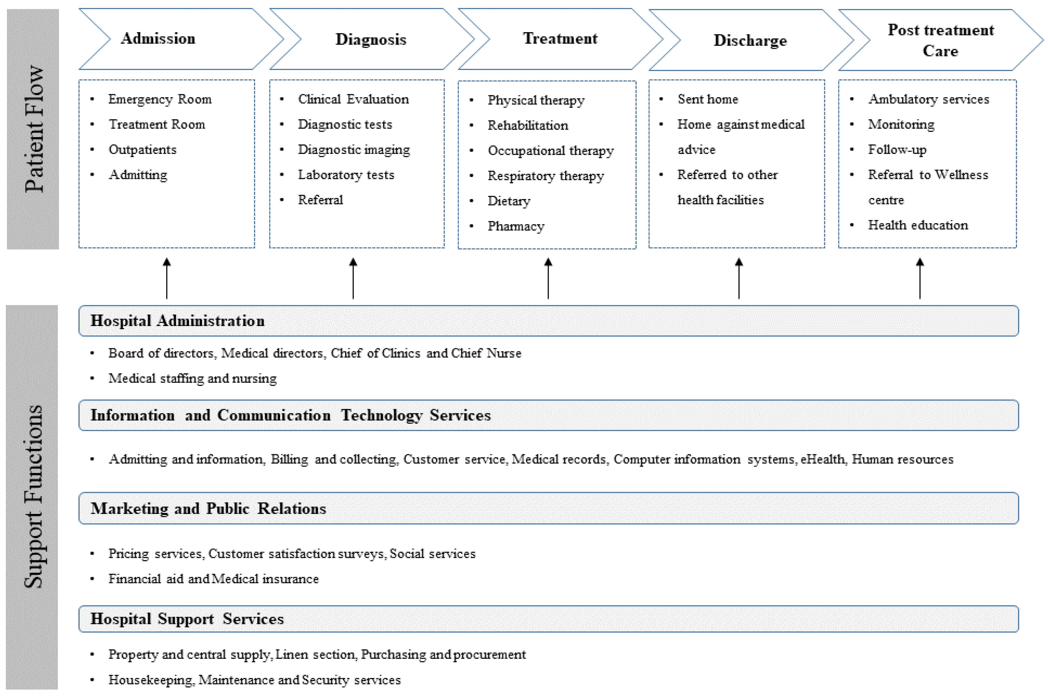
The authors commence the research by defining the activities at a healthcare facility, specifically a typical hospital, with particular focus on how activities associated with maintenance relate to the entire organisation. Lee et al. [34] describe the criteria for classifying hospital types and their functions, including primary care hospitals, secondary care hospitals and tertiary care hospitals. A secondary care hospital, for example, typically has over 100 beds, and acts as a referral centre for primary medical institutions. It also operates the 9 fundamental departments including general surgery, paediatrics, obstetrics, radiology, psychiatry, etc. Figure 1 indicates the value-chain framework typical of a generic primary or secondary care hospital, with the key activities structured according to the stages that patients pass through during treatment [35]. According to the framework, facility maintenance and management is identified as part of the support service functions within the hospital [36].
The maintenance process is then mapped in MS Visio using data collected from public and private hospitals in South Africa. The asset register, MTBFs and resource lists, as well as equipment specifications and criticality, are then entered into structured query language (SQL) databases and migrated into MySQL Workbench 8.0. Figure 2 indicates the entity relationship diagram of the maintenance system’s components from within the MySQL Workbench application. As indicated in the figure, the key components of the system include spare parts, maintenance tasks list, equipment list and personnel. The tables for breakdowns logged, generated maintenance jobs and spare parts inventory are populated because of the interactions of the key components listed above. The yellow tabs in the figure represent query tables for metrics of interest. The developed database management system provides the researchers a means with which to capture and store the various streams of data and information within the maintenance system. The database system is also used to store the specific step-by-step maintenance instructions than must be followed in executing maintenance tasks, along with standard times for the task durations and an indication of all resources that may be required, such as spare parts and shared workshop tools. Structuring these data into a relational database system ensures that all activity relationships are considered and defined for the modelling phase.

3.2.2. Build Process Model and Translate to Digital Model

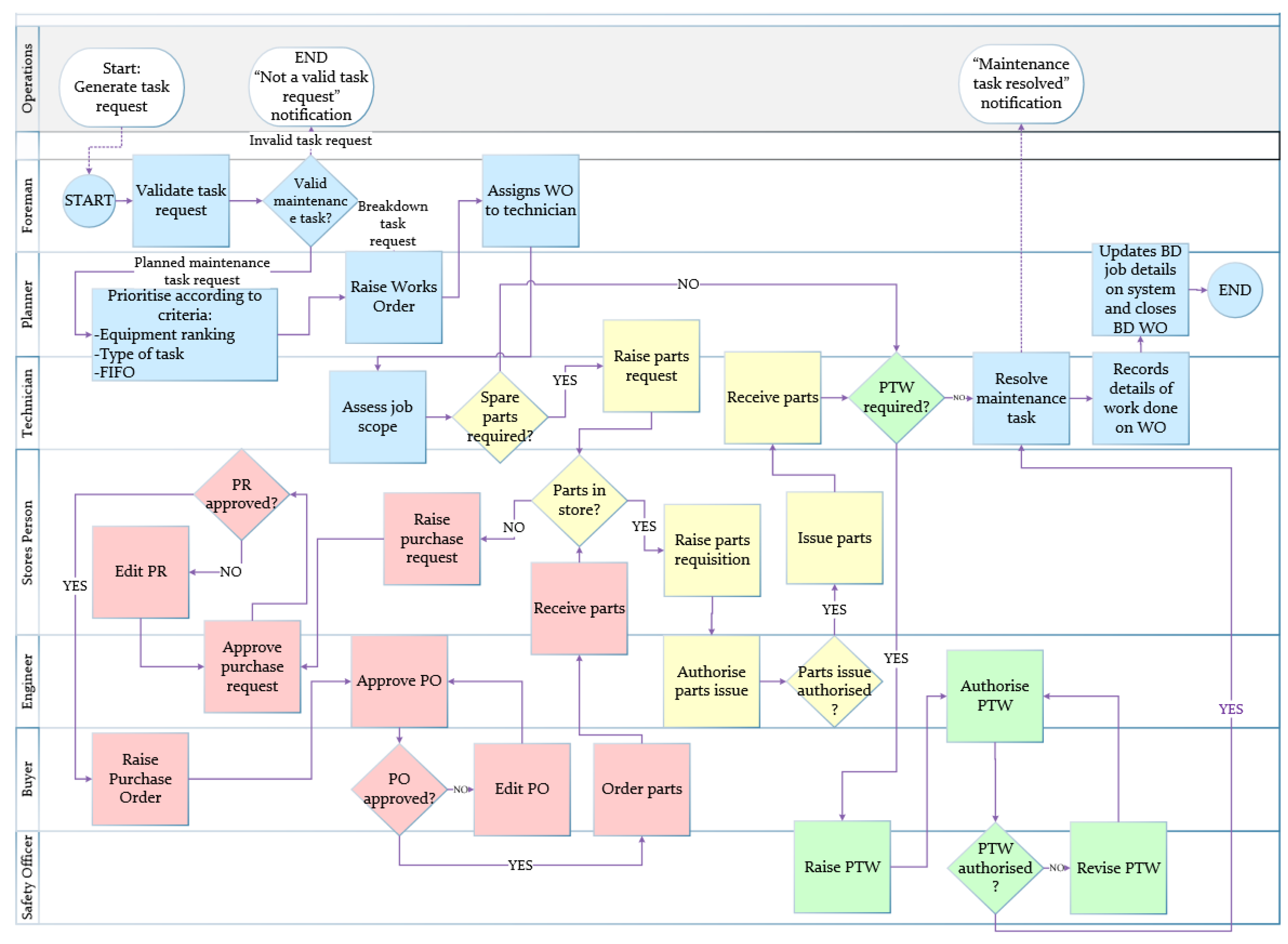
Figure 3 indicates a process flow model that describes the maintenance management system. After maintenance task requests are generated, the maintenance supervisor first validates them by checking with the user departments or with the maintenance planner before routing them accordingly. Validated planned maintenance tasks are scheduled according to set prioritisation criteria before they are released and assigned to technicians for execution. The prioritisation criteria consider equipment ranking, as well as type of task and order of arrival into the queue. Breakdown tasks are routed differently and are treated as emergency works orders. All types of maintenance tasks, however, namely corrective maintenance, preventive maintenance and predictive maintenance tasks, go through similar steps once they have been assigned to technicians for execution. The jobs may or may not require spare parts and specialised tooling from the store and the central workshop, respectively. If spare parts are required but unavailable, the procurement process is triggered while the respective task waits in queue. In Figure 3, the blue shapes represent the flow of the main maintenance activity, while the yellow part represents the process of parts requisition and issuance. If the required parts are not available in the engineering store, the procurement process is followed, whose flow is as indicated by the red shapes. Finally, the green shapes indicate the process steps related to safety procedures that must be followed when a permit to work (PTW) is required for the maintenance task.
After establishing the maintenance process flow and setting up the database for maintenance data, the Python programming language and its SimPy library for discrete event simulation are then used to extend this setup into a digital model. The approach adopted gives the model flexibility to accept a practically unlimited number of asset groups and asset units. Both DES and SimPy have been in use building simulations for a wide variety of scenarios for more than 20 years. SimPy is a process-based DES framework based on standard Python language. Python and SimPy provide a solid basis for the object-oriented programming tools needed to build models and run the simulations. Matloff [37] and van der Ham [38] explain the working of both tools to sufficient depth. Alrabghi & Tiwari [15] discuss queuing approaches to DES modelling within a maintenance context.

3.2.3. Define System Variables

Guided by the objectives of attaining target service level and operating cost optimisation, the relevant system variables are identified. Based on the process mapping, an analysis of all system variables is carried out to determine the dependent, independent and control variables. Out of the identified independent variables, the researchers designate as variables of interest those variables that are typically within the direct control of the terotechnology practitioner; namely:
  • maintenance strategy per equipment group (that is, maintenance type and frequency);
  • spares inventory stocking and replenishment policy; and
  • human resources.
Unit costs, however, are considered extraneous control variables that must be kept constant so that they may not serve as confounders in the study. A list of all identified system variables, listed by type, is given in Table 1. In addition to maintenance frequencies, the independent variables that relate to system resources, namely, equipment, people and spares, are incorporated into the solution set as decision variables by which the system is to be optimised. A total of 4 + 2 n decision variables are identified, where n is the number of asset types in the system. The system’s overall objectives are encapsulated in 3 of the operation-related dependent variables, namely, customer service level, operating margin and productivity. Actual customer service level is assumed equivalent to overall equipment availability and this is compared against a benchmark customer service level target in healthcare facilities of 85% [4].

3.2.4. Define Bounds and Constraints

In order to improve efficiency of the search, the solution space is confined by defining practical ranges for the respective decision variables and specific values for the control variables. Lower and upper bounds for the decision variables are specified based on empirical knowledge of the maintenance system [15], or as determined by physical limitations imposed by the system. Values specified are from an actual healthcare facility in South Africa.
Resources: we define 4 non-equipment-related decision variables for the system, namely: number of technicians, N T E C H ; spares reorder quantity, Q O R D ; spares reorder level, Q R E O R D ; and spares maximum level, Q M A X . The decision variables constitute the solution set for optimising output and the following bounds are defined. The range for N T E C H is based on the human resources policy for the organisation and, in the considered case, the number of technicians hired varies between 1 and 10. In addition, due to physical space constraints in the spares store and due to other considerations, such as financial policy and security risk, minimum and maximum limits to spares stock holding apply. In this case, quantity of spares in the store may vary between 0 and a maximum of 500 units. The reorder level may be any point between 0 and 300 units. Minimum and maximum reorder size is constrained by factors including nature of supplier, buying policy and lead-time considerations. We consider a case when Q O R D may vary between 10 and 200 units. The reorder quantity and reorder level ranges for spare parts are selected such that stores spares inventory may not exceed Q M A X . The instantaneous inventory level in store is Q L V L .
1 N T E C H 10 0 Q R E O R D 300 10 Q O R D 200 0 Q L V L Q M A X , w h e r e   Q M A X = 500
Maintenance Frequencies: in addition, for each asset type, we identify 2 decision variables to consider for each asset type i , namely, time between preventive schedules and time between predictive schedules, T P R E V i and T P R E D i , respectively. The scheduled times between preventive maintenance tasks and predictive maintenance tasks are deterministic since they are planned and executed at predetermined periods. For all equipment types in the case study, preventive maintenance schedule frequencies vary between 1 schedule per 4-week period (most frequent) and no schedules at all in the simulation period (least frequent). Similarly, predictive maintenance schedules have a maximum frequency of 1 schedule per week and a minimum of 0, that is, never. The maintenance frequencies stay the same within an asset group, but may vary between asset types. If time in operating period is T O P weeks, then:
4 T P R E V i T O P + 1   [ w e e k ] 1 T P R E D i T O P + 1   [ w e e k ]
Control Variables: the control variables have a bearing on system performance but remain constant throughout the simulation period. We identify at least 15 control variables that must be specified at the start of the simulation (see Table 1). Values for the control variables are specified as below.
Resource-related control variables: for staffing and spares resources, we define the following control variables. Absenteeism is used to determine full time equivalents (FTEs) and related productivity performance indicators. Maintenance activity on asset j of type i may consume S i j spares, where S i j randomly varies between 0 and 2. For costs, we specify average unit cost of spares and daily rate for labour. Typical of pay systems in use throughout the developing world, a flat daily pay rate for technicians is assumed, whether they have worked full hours or not.
Absenteeism rate , A = 0.1 Spares lead time , L = 3   d a y s Spares consumption per task , 0 S i j 2 Labour cost per technician per day , C P D = $ 6.60 Spares cost per unit , C S U = $ 15.00
Equipment-related control variables: the values for T B D i assume no maintenance interventions. Values specified are based on statistical analysis on the collected data. Breakdowns are defined as work stoppages greater than 10 min, so that any stoppage lasting below that period is considered a minor stop. Service tasks due on equipment that is already down are counted but considered un-executable and therefore skipped. This is in line with accepted industrial practice where equipment in the workshops for other repairs is not separately serviced even if due. Predictive maintenance activity duration includes time for any follow-up basic condition restorations.
M e a n   t i m e   b e t w e e n   b r e a k d o w n s   f o r   a s s e t   t y p e   i , 4 T B D i 39   [ w e e k s ] M e a n   p r e v e n t i v e   m a i n t e n a n c e   d u r a t i o n , μ P R E V = 150 , v a r i a n c e σ P R E V = 30   [ m i n u t e ] M e a n   p r e d i c t i v e   m a i n t e n a n c e   d u r a t i o n , μ P R E D = 50 , v a r i a n c e σ P R E D = 12   [ m i n u t e ] M e a n   b r e a k d o w n   m a i n t e n a n c e   d u r a t i o n , μ B D = 90 , v a r i a n c e σ B D = 25   [ m i n u t e ]
Equipment quantities: the tool is designed such that it can handle a practically unlimited number of asset types and assets. However, in order to ensure manageable execution times, the program requires the researchers to specify the minimum and maximum quantities per asset type. The program, within the limits specified, then generates the actual number of units for each asset type. Regardless, the researchers may overwrite the default behaviour and explicitly define the quantities of asset groups and units per each type with which they wish to do the simulation run.
Number   of   asset   types , 1 n i 10 Number   of   m   per   asset   type n i , 0 m j 10
Operations-related control variables: we consider a 52-week planning horizon. Beyond planning, operational data such as operating hours and running pattern are usually beyond the terotechnologist’s scope of control. Accordingly, in line with common operational patterns within the healthcare sector, we consider an operational pattern of 24 h per day and 7 days per week. Depending on the shift system in use, the number of technicians that the tool suggests must therefore be multiplied by the number of shifts per 24 h in order to give the actual headcount. We assume an infinite customer population such that the customer service level, S L A C T , may be considered to be in direct proportion to equipment availability. The target customer service level, S L T G T , is as determined by organisational policy. We define the downtime cost, C D T , for asset m i j as that cost that must be incurred, over and above the costs of labour and spare parts, in order to make the asset operational again. It may include logistical costs, equipment hires and tooling costs among other components [39]. Finally, the researchers specify operations-related control variables as follows.
O p e r a t i n g   t i m e , T O P = 52   w e e k s × 7   d a y s × 24   h o u r s T a r g e t   c u s t o m e r   s e r v i c e l e v e l , S L T = 85 % U n a v a i l a b i l i t y   c o s t   p e r   a s s e t   p e r   h o u r , C D T = $ 2.50   p e r   a s s e t   p e r   h o u r G r o s s   r e v e n u e   p e r   a s s e t   p e r   h o u r , R A S T = $ 2.50   p e r a s s e t p e r h o u r
Dependent Variables: the system has more than 10 output variables that give indication of the system’s performance. The key performance indicators include overall customer service level, S L A C T , operating margin, P , as well as productivity rate, queue delays and number of breakdowns.

3.2.5. Formulate Objective Function

We may now formulate the objective function as:
m a x i m i s e   P = R C L C S C D T
subject to the following constraints:
1 N T E C H 10 0 Q R E O R D 300 10 Q O R D 200 0 Q L V L Q M A X , w h e r e   Q M A X = 500
and
4 T P R E V i T O P + 1 1 T P R E D i T O P + 1 , w h e r e   T O P = 52 a n d   1 i n
where:
t o t a l   r e v e n u e   g e n e r a t e d   i s   g i v e n   b y : R = w e e k = 1 T O P i , j n , m R A S T i j t o t a l   l a b o u r   c o s t   i s : C L = N T E C H × C P D t o t a l   s p a r e s   c o s t   i s : C S = C S U × i , j n , m S i j × N T O T , a n d t o t a l   u n a v a i l a b i l i t y   c o s t : C U = D × C D T
where N T O T and D represent the total number of maintenance tasks generated and total downtime in the period respectively, and they are determined as follows:
Number of tasks: let m i denote the number of units of asset type i, and let n denote number of asset types. Task inter-arrival rates are determined from mean times between successive tasks:
λ B D i = 1 / T B D i λ P R E V i = 1 / T P R E V i λ P R E D i = 1 / T P R E D i
Therefore, if operating period is w weeks, then number of tasks generated is given by: T o t a l   m a i n t e n a n c e   t a s k s   =   u n i t s   p e r   a s s e t   t y p e   ×   t a s k   g e n e r a t i o n   r a t e   ×   p e r i o d , that is:
N T O T = w × i = 1 n ( m i · 1 T B D i ) i + i = 1 n ( m i · 1 T P R E V i ) i + i = 1 n ( m i · 1 T P R E D i ) i
Total downtime: total downtime is given by:
D = j , k = 1 m , n m j k · t r e p k + j , k = 1 m , n m j k · t p r e v k + j , k = 1 m , n m j k · t p r e d k
where:
  • t r e p k is the mean time to repair asset of type k, including queuing time;
  • t p r e v k is the mean time to execute a preventive schedule on asset of type k, including any waiting; and
  • t r e p k is the mean time to execute a preventive maintenance schedule on asset of type k, including queuing time.

3.2.6. Set Up the Discrete Event Simulation

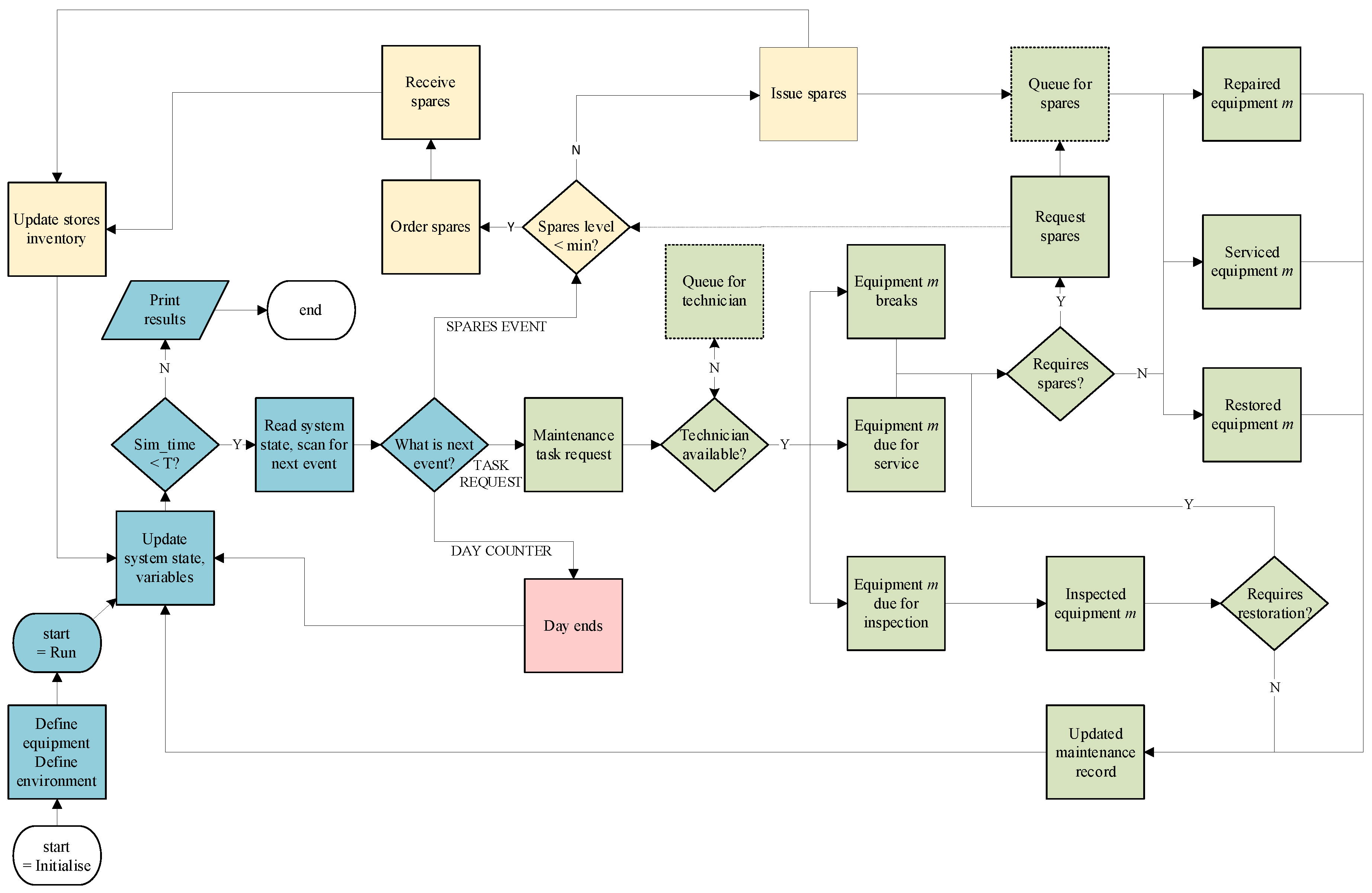
Simulation is chosen as the most practicable scientific approach in this study due to the complexity involved in using other methods. For example, use of an analytical approach would require making too many assumptions in order to arrive at a solvable objective function. Moreover, the availability of standard computational power now allows for simulation modelling for problems such as optimisation, what-if analysis and sensitivity estimations, goal seeking in the design analysis and control of processes that were previously beyond reach of decision makers [7]. However, using systems modelling and simulation requires an understanding of both the technique of simulation modelling and of the simulated system itself. The details of the discrete events that occur within the model are as indicated in Figure 4. Within the DES model, the researchers are interested in resources-related independent variables as well as planned maintenance frequencies since they are directly controllable from the perspective of maintenance management. Accordingly, the solution sets generated by the program comprise number of technicians, starting inventory, reorder level and reorder quantity, as well as service- and condition-monitoring frequencies.
The starting values for each of these parameters, which collectively comprise the initial solution, are taken from the current operating parameters of the system under study and are read directly by the Python script from the MySQL database. Alternatively, these values may be generated randomly within specified ranges as derived from case study data, subject to limitations and constraints imposed by the process characteristics of the system. In respect of MTBF data, the probability of equipment failure for each asset type is considered to rise exponentially with time, in accordance with the Markovian probability distribution function. It is assumed, however, that the distribution profiles for repair, service and restore data all follow a normal distribution curve, such that a mean and standard deviation are required in order to define time profiles fully. Minimum and maximum periods between services or repairs are also specified in line with defined variable bounds. Actual parameter values for preventive and predictive maintenance intervals are either based on empirical data from case studies or left to the program to sample the starting service intervals for each equipment type randomly.
DES Performance Evaluation: statistical methods are used for output data processing and results analysis. Total cost and gross margin are used to calculate an operating margin, which represents the system’s energy state and overall performance. The customer service level is calculated based on asset uptime, whose relevant data are obtained from downtime logs generated during the simulation runs. Other useful system performance metrics to output include queue performance data, such as average queue length, total slack, task backlog, queue waiting times and total number of tasks active in the system at a given point. Average server utilisation, given by λ/µ, where λ is the queue arrival rate and µ the mean server process time per task, indicates the capacity utilisation of the system. A processing time, µ, that is less than the task generation rate, λ, indicates a constrained system, and long task queues may eventually form. A task generation rate that is too small indicates underutilisation of the system’s resources.
Other Assumptions: it is assumed asset failures follow the Weibull exponential probability distribution curve. According to Sánchez-Barroso & Sanz-Calcedo [40], the Weibull distribution is the most preferred assumption used by researchers seeking to model equipment failures in maintenance process models. As Sánchez-Barroso & Sanz-Calcedo explain, given the right shape co-efficient, this distribution has been empirically proven able to predict when equipment failures will occur during operation relatively accurately. However, since failures have an apparent randomness to them, the Monte Carlo distribution assumption is also sometimes preferred, particularly in cases when there is deemed to be a weak correlation between probability of failure and any preceding maintenance interventions such as inspections [40]. As the failure probability distribution is exponential, we assume that interventions have the effect of restarting the probability curves so that the breakdown clock is effectively reset.
On queue discipline, we assume there is no baulking and no reneging since this is a queue of inanimate maintenance tasks. In maintenance systems, tasks may eventually be outsourced when stuck for too long or they may be written off. Nevertheless, here it is assumed that all tasks in the queue will remain so until resolved. Otherwise, they reflect as backlog. It is also assumed that task arrivals from the different assets are all independent of each other, being governed only by the respective probability distributions within their own machines. Finally, we assume that service times per task are independent and that the maintenance system operates under steady ongoing conditions, and that arrival and service rates remain stable throughout the simulation.

3.2.7. Set Parameters for Simulated Annealing

With all parameters for the DES model specified as discussed, the program is ready for simulation runs. Multiple runs using various data sets afford the researchers an opportunity to test the tool’s robustness and performance. The program can be used in this state as a standalone tool for analysis and system insights. However, additional benefits are realised when the DES is implemented in conjunction with the SA algorithm such that automated optimisation is possible. The SA algorithm is selected as it is a proven heuristic that has been applied in several optimisation problems, and recent examples within maintenance management are available [41,42,43]. According to Ali et al. [44], SA is a direct search approach that is well suited to global optimisation problems that do not require differentiability or any other special properties for the objective function, such as determinism and no noise. Even though it does not always find the best solution, it provides for Pareto optimal solutions for applications such as the problem considered in this study. It is only necessary to generate a good quality solution and not necessarily to find the global optimum since the operating environment is dynamic. The DES model is ‘inserted’ into the SA algorithm in the place of the objective function, as shown in Figure 5.
As usual, we begin the SA algorithm with an initial solution, which, in the case of the maintenance problem, is the set of numbers representing the level of spare parts inventory maintained in the store, number of technicians and the frequency of planned maintenance work orders, for example. We then use that solution set to determine the energy value of the function, E , whose minimisation is our objective. This energy value takes into account the overall maintenance cost associated with this solution set, as well as the equipment availability and efficiency. We then follow the criteria for selection of a random neighbour to the current best solution and compute the energy associated with this neighbouring solution. The function of the DES module in this case is to carry out the stochastic computation of the E values, which are subsequently passed into the SA algorithm for comparison and selection or rejection, in line with the SA algorithm’s design. This allows for the repetitive running of the DES model and the automatic evaluation of its outcomes. This is an improvement over previous works in which the ‘handshake’ between the DES module and the optimisation algorithm had to be done by hand, for example Alrabghi & Tiwari [15]. A global optimisation heuristic is applied to analyse results of the DES and to find optimal solutions. Visualisation of the simulations and performance are depicted through graphs.
Simulation Parameters: in order for the SA algorithm to operate effectively, it has a set of parameters that must be specified correctly. These are the starting and final temperatures, cooling schedule, number of iterations and any convergence criteria. Table 2 indicates the simulation parameters and corresponding values used in this study.
During the search for a global optimum solution, the DES simulation is run multiple times within the SA algorithm as determined by the simulation parameters specified, as shown in Table 2. All parameters shown are critical to the efficiency of the search and the quality of solutions [45,46]. Due to the need to balance efficiency with performance between the DES and SA modules, the researchers set the number of iterations per temperature step at 50 runs.
Cooling Schedule: the cooling schedule is crucial for the quality of the search [47]. Two cooling-related critical factors here are the initial temperature and the cooling rate. There is not much literature on investigating how to determine a good initial temperature, but such a temperature should permit solution space exploration by yielding a high initial probability of accepting bad moves. This threshold is generally taken to be at least 0.8, and then the probability of acceptance of bad solutions may decrease with decreasing temperature [48]. The ideal cooling function and final temperature allow for the exploitation of good neighbourhoods within the search space. Accordingly, we define the initial temperature according to a function based on the simulation period, number of machines and gross revenue. We also choose a final temperature, T f , that ensures an adequate number of cooling steps. This value, together with the cooling factor, α, must be such that the cooling does not proceed too fast and end prematurely. We adopt an exponential cooling function with α = 0.75, which ensure iterations over at least 40 temperatures between T 0 and T f . The cooling curve obtained with these parameters indicates that a stable temperature (ambient) is reached after just 18 to 20 steps. This compares favourably with other cooling schedules used by other researchers, which typically reach a stable entropy at about 21 to 23 steps into the simulation [45].
Solution Space: apart from the initial cooling temperature and the cooling schedule, another intervention that helps to optimise the search algorithm is the search strategy adopted for finding candidate solutions from the search space neighbourhood. This is due to the large number of points within the solution space, which renders the optimisation computationally expensive. For example, we consider that the number of decision variables for n asset types is given by 4 + 2 n , where n is the number of asset types. Since the solution space size is a function of the number of decision variables, as well as the range of each decision variable, given the variable bounds specified in this study, we may determine the size of the solution space as follows:
S i z e   o f   S o l u t i o n   S p a c e   =   10 × 501 × 191 × 301 × 50 × 53 × n = 763279261500 · n
where n is the number of asset types in the system.
Accordingly, for a facility with, say, 10 different asset types, the number of decision variables is 24 and the solution space size will comprise above 7.6 trillion solution sets, hence the need to optimise the search algorithm.
Solution Space Search Strategy: accordingly, the researchers adopt a solution space reduction (SSR) strategy that progressively delimits a smaller and smaller active search space within the global solution space as the system cools down to a stable entropy value. The chosen strategy is based on a number of variations that have been demonstrated to improve the efficiency of the search and accuracy of results [46,49]. A form of dynamic SSR, called hull form optimisation, works by using data mining to reduce the range and number of variables continuously, only enabling subsequent optimisation steps in ranges where high performance is indicated, thereby reducing calculations and improving efficiency and accuracy [49]. In the present study, however, authors only implement range reduction but maintain all variables since they are of equal interest in healthcare maintenance optimisation. They further build on the work of Mahesh & Sushnigdha [46] to formulate a solution search method that negates the need first to check if a candidate solution violates boundary limits, thus gaining a small improvement in efficiency.
Figure 6 indicates how this logic is implemented. For successive candidate solutions as the cooling schedule progresses, the selection of neighbouring solutions is still random but is now further constrained in range by a function dependent on ratio of current to initial temperatures. The general principle of solution space reduction strategies is that, while at higher temperatures, most or all of the feasible solution space is explored, and the neighbourhood of candidate solutions is made progressively smaller around the current best solution as the system cools. In this way, the risk of losing good solutions is minimised while at the same time ensuring that the system can break away from bad solution spaces. In the diagram, S 0 represents the initial solution, which can be anywhere within the feasible solution space, A, as well as all other candidate solutions that can be selected and tested while the temperature is still at T 0 . Once the next temperature step, T 1 , is reached, the solution, S 1 , is initially determined based on S 0 but will now have a smaller neighbourhood for successive candidate solutions. Solution spaces C, D and E show that, regardless of the location of the solution within the global solution space, the range of the accessible next solutions stays the same as long as the temperature step remains unchanged. The movement of the current best solution from S 3 to S 5 through S 4 indicates how a point that may not be directly accessible can still be reached via intermediate solutions. This mechanism ensures that the search does not stay trapped inside a bad solution neighbourhood, so long as the entropy is still sufficiently high to allow the jumps.
Incorporating the DES module: the SA metaheuristic can be used to find either global maxima or minima. In a maximisation problem, as in this study’s case, the following logic applies. If the newer energy value, say E 2 , is higher than the older energy value, say E 1 , then E 2 is accepted as the current ‘best energy value’ and the solution set that produced it becomes solution S b e s t . This new ‘best solution’ is then used to determine the new solution space’s local neighbourhood (see Figure 5) and as the basis for determining the next candidate solution. The set of input parameters that produced E 1 is discarded. However, even when the new value, E 2 , is not less than E 1 , it may still be accepted and its input solution set adopted as the ‘best solution’ with a probability that is determined by the Metropolis criterion. This criterion computes the value of e raised to the power of —(∆E/T), where T is the current system temperature, and then compares this value to a randomly generated number between 0 and 1. If the metropolis value is greater than the random number, the worse energy value is accepted; otherwise it is rejected. Therefore, the probability of acceptance for bad solutions depends on the difference in energy levels between E 2 and E 1 and the current system temperature of the simulation, T , as well as on an element of randomness.
The larger the energy difference or the smaller the temperature, the less likely a bad solution is to be accepted. Conversely, the smaller the difference in energy levels of the two solutions or the larger the temperature, the more likely a bad solution is to be accepted. This dynamic encourages wide exploration of the search space early on in the simulation, but, as the system continues to cool, the likelihood of movement towards worse solutions is reduced, thereby increasing the chances of locating the function’s global minima and settling in it. Figure 5 indicates the flow of logic in the SA model, with the DES module (shown in full in Figure 2) inserted. The role of the DES module in this setup is to work as the objective function that generates the E values from candidate solution sets provided by the program.

3.2.8. Execution

To build the solution, an analysis of the maintenance workflow is first carried out and used to develop a digital maintenance management model with m equipment types, each of which could have up to n units. Each workflow may generate one or more of up to three types of task requests and route them to a central server for resolution. The workflow model is then translated into a DES. This simulation is then further built into a SA metaheuristic in lieu of the objective function. The SA algorithm then facilitates the multiple testing of the DES and searching for a global optimum in the solution space. The program is tested using empirical data from selected healthcare facilities in South Africa. Predictions and recommendations from the simulation runs are compared with historical performance data in order to validate the model, and are analysed for insights, which are then given as recommendations. Finally, the complex relationships between input parameter sets and key performance indicators, including costs and service levels, are explored and discussed.

4. Results

The main aim of this study was to develop a tool for assisting healthcare maintenance and facility managers in low-income economies to run their facilities more effectively at optimum levels of customer service and costs. This aim was achieved by determining the set of independent resource variables that ensures optimum performance. The relevant performance objectives were maximising customer service level, minimising maintenance cost and workflow optimisation. To evaluate the tool’s performance, multiple cycles of the simulation were run, and a sample screenshot of output from the 52-week DES simulation is presented in Figure 7. The simulation was conducted using input data from a healthcare facility with a moderate level of asset heterogeneity, consisting of 49 assets in 10 asset groups, and was performed using Python 3.8 in a Spyder IDE (integrated development environment).

4.1. Initial Conditions

The facility at which the tool was tested is a hospital whose maintenance department employs three technicians, one per each 8 h shift. Initial spares inventory in store was 100 units, with a reorder level of 10 and a reorder quantity of 50. The equipment parameters for the initial conditions are as indicated in Table 3.
Based on this set of initial conditions, the program determined the corresponding level of performance of the system by running the DES once. This was an important step as it provided a benchmark against which final results were compared. Thereafter, the simulation and optimisation loop was run multiple times, and the final output obtained was as follows.

4.2. Output

Figure 7 is a collage of screenshots of the initial conditions and the final results. The results include a summary of the changes in key performance indicators (KPI) between the initial solution and the final optimised solution. The program was set to simulate a 52-week operation, and program execution took 12 h and 52 min before it could produce the final output. Based on the changes in the KPI values, it was observed that the program was able to find an optimum solution that significantly improved operational performance of the system, with an increase in profit margin of 64%, a reduction in breakdowns of 22% and a marginal improvement on an already high customer service level.
Figure 8 indicates the number of maintenance tasks by type, as well as task durations versus queue delays before and after optimisation. The total count of maintenance tasks increased by 23% as the system introduced preventive maintenance schedules into the system and increased the frequency of predictive schedules. These increases in preventive schedules (from 0 to 40) and in predictive schedules (from 83 to 143) caused an overall reduction in breakdown frequency per week (from 3.42 to 2.65). As a result, downtime cost was reduced from USD 7000 to USD 2000, while the overall maintenance cost was reduced from USD 15,971 to USD 12,426. There was also an 80% overall reduction in job delays, which was reduced from 2454 h to 502 h over the 52 weeks.
Figure 9 indicates the spares inventory time trends as well as the overall costs at the start of simulation and after optimisation. While there was no significant change in the initial level of spares between the initial and final solutions, it is observed, however, that the reorder size was smaller in the optimised solution, suggesting that smaller but more frequent purchases were more optimal. This is in line with the relatively short lead time of 3 days used in the simulation. The program also selected spares inventory parameters such that the purchases were more frequent in the second half of the year than in the first, coinciding with the period of increased maintenance activity.
The overall costs graphs show a 20% reduction in maintenance costs. At cost-component level, however, there was no change in the level of staffing between the initial and the final solutions, meaning that labour costs stayed the same. The cost of spares was higher in the final result due to increased planned maintenance activities, which resulted in higher spares consumption. Nevertheless, the increase in spares cost was more than made up for by the significant reduction in the cost of downtime. Overall, downtime was the biggest cost component of maintenance costs before optimisation. After optimisation, however, the spares cost became the most significant contributor to the maintenance cost.

4.3. Search History

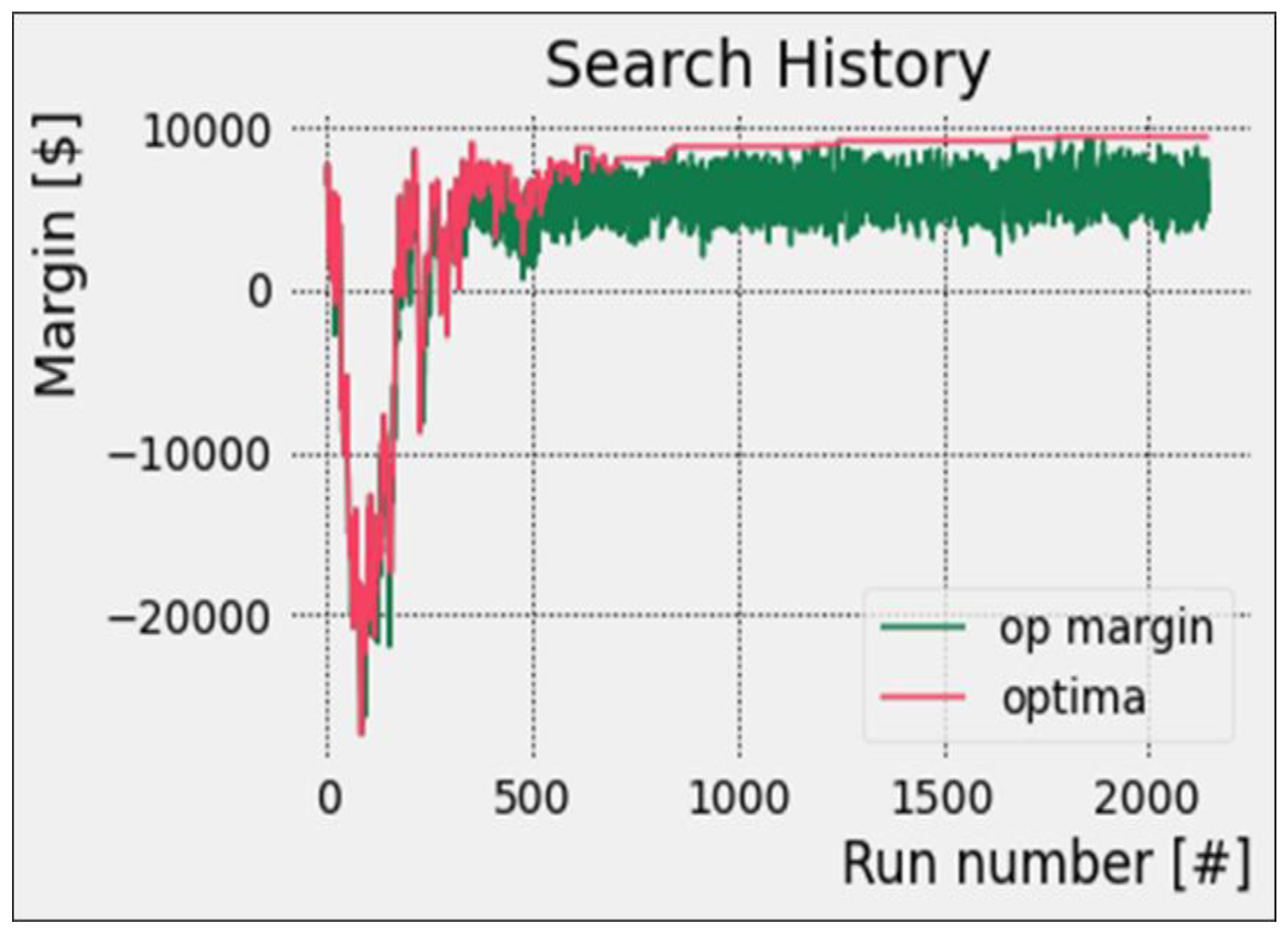
Finally, Figure 10 shows the optimisation search history across over 2000 runs. Within the first 500 simulations, the algorithm accepted significantly worse moves as it explored the search space. Thereafter, for the next 200 to 500 simulations, the solution quality steadily improved in small steps as the algorithm exploited good solution neighbourhoods. There was only a marginal improvement in the solution quality beyond 1500 simulation runs.

4.4. Analysis

The visual results obtained give some insights into the system’s performance. For example, the spares cost in Figure 9 increased markedly in the second half of the year as more preventive maintenance schedules became due. Since breakdowns have priority over other task types, and since resources are apparently limited, it is observed that the resources focused on the breakdowns whose frequency was also beginning to increase in the third quarter due to inadequate maintenance. After a gradual stock level decline due to very little maintenance activity in the first quarter, the frequent spares reorder cycles started in the second quarter. Clearly, the delay spike at about 4300 h (that is, at about 180 days) was due to a spares run-out. It can be deduced from the trends that, even though the operation had only one technician, the delays were not due to skilled labour shortage, but rather to abrupt spares run-outs. The store’s inventory time trends before and after optimisation (Figure 9) indicate an optimisation of the spares management policy. Figure 9 indicates a 100% increase in reorder points and a corresponding order quantity reduction of 20%.
As indicated in Figure 7, in addition to the output graphs, the simulation also gives a textual summary of the system’s performance in the simulation period. The information includes asset input data, a task’s performance summary and cost performance data, including the operating margin. By searching for an optimum solution, the optimisation module was able to improve the operating margin by 64%. Although the cost of spares marginally goes up, the overall maintenance cost is reduced by 20%. In addition, the service quality is enhanced as overall queue delays are significantly reduced. The simulation shows that a higher spares reorder point, coupled with a smaller but more frequent order quantity, leads to a higher service rate than a lower reorder point with bigger and less frequent orders. Since the initial solution was from a real case, this means that the tool is able to find solutions that significantly improve maintenance operations.

5. Discussion

This study sought to provide a simple and cost-effective means of determining optimum maintenance strategies in an objective manner, and in line with relevant operating parameters, such as the number of machines and machine types, MTBF and MTTR data, service schedules, spares stock levels and lead times, and operating times. We proposed a decision-support tool that combines DES and SA in a novel way, building upon the modelling approach of Zhang [31]. One key feature that distinguishes this model from previous ones is its full autonomy. For example, the previous model developed by Petroodi et.al [33] relied on manual intervention in the manipulation of output between the DES module and the complementary metaheuristic.
The developed tool comprises a DES core encapsulated inside an SA metaheuristic. The DES module simulates the operations environment and provides the means of correlating multi-factor input parameters to system output values. The SA algorithm then takes the respective sets of process input and output parameters as candidate solutions and checks for optimality. It progressively seeks and accepts mostly better solutions within the current solution’s neighbourhood, thereby exploring the entire bounded solution space until convergence is obtained. However, a critical consideration of the search history trend reveals that, while more simulation runs generally lead to better solution quality, there is a point beyond which the gain in solution quality is no longer significant enough to justify the additional computational cost. Accordingly, it is important to identify this threshold in practical implementations of the tool if unnecessary additional computational costs are to be avoided. Simulations carried out in this study suggest this threshold to be somewhere between 1000 and 1500 simulation runs.
The approach used in this study demonstrated a clear and logical methodology for developing a robust generic two-module maintenance decision-support tool. The tool developed is able to:
  • determine what the input parameters must be in order to ensure optimal performance, not just of the maintenance function but of the health facility in general, including operating margin and customer service level;
  • determine the optimum frequency for preventive maintenance activities on a given asset;
  • show visual outputs that can be studied for insights and that may reveal hidden relationships among variables;
  • give information that can assist managers to formulate a store’s spares policy that is in sync with operations and maintenance;
  • provide what-if analysis feedback that managers can use to improve the quality of strategic and tactical decision making; and
  • work in any facility with discrete assets without any further customisation.
The model’s output suggests that predictive and preventive schedules must be built into maintenance strategies at specific levels in order to optimise costs and equipment availability; that is, the precise number of the respective schedules must be determined, as well as when they must be executed. These findings are in harmony with earlier conclusions drawn from the work of Carnero and Gomez [26] who, in a maintenance optimisation study of heating, ventilation and air-conditioning (HVAC) equipment within a medical facility, concluded that combining predictive and condition-based maintenance would lead to the most effective strategy. The results obtained in our study indicate cost savings of up to 20%, mainly driven by a reduction in equipment downtime. This outcome appears to compare favourably to the savings of 14% achieved by Pargaret al. [7], who used an integer-programming based approach. However, as the case of Pargar et al. [7] is in a significantly different business context, it would be necessary first to reproduce their model and test it with our data before any definite parallels can be drawn between the two respective models, and this, therefore, is an opportunity for further work. However, besides the apparently lower savings, Pargar, et al.’s model was not capable of handling heterogeneous equipment mixes as the model proposed in this study does. On algorithm efficiency, results obtained indicate that the modified solution space reduction strategy applied here leads to an improved search efficiency. This outcome is consistent with the findings of Mahesh and Sushnigdha [46].
Validation of the model was done with actual case data from the maintenance department of a public hospital. The hospital was faced with the key challenge of how to improve reliability and availability of critical ventilation, refrigeration and related machinery quickly and cost-effectively, in the face of an increased strain on the equipment caused by a spike in COVID-19-related admissions. The model demonstrated the capability to handle complex machine mixes, and the test case used had 49 machines falling into 10 equipment groups, each with different maintenance requirements, priorities and parameters. Some key variables, for which the program could help determine optimum levels, included labour and spares, as well as the overall running strategy for the maintenance management system.
Although the model was validated using real case data, time constraints prevented us from fully addressing other challenges that could emerge during implementation. For example, whereas the program might suggest a solution with reduced labour and increased spares inventory, implementation of such measures must take into consideration the human resource policy of the institution, as well as the impact on short-term liquidity, respectively. Therefore, it is recommended that the output be used as a mere objective indicator to point towards the right direction in the decision-making process, rather than being taken prescriptively.
One of the major challenges that could arise during implementation of the decision-support tool is that the inertia of staff accustomed to traditional ways of working could adversely impact effectiveness of the tool. Another challenge is that successful implementation would require technical expertise in the areas of modelling and simulation during setup, and this may not always be readily available. However, once the tool is setup, only basic skills would be required for day-to-day use. Yet another implementation challenge is that integrating the tool into existing maintenance management systems could pose significant challenges if those systems are outdated or incompatible. Finally, since the quality of the output is dependent on the accuracy and completeness of the data used as input in the decision-support tool, if the data quality and availability are poor, this could adversely impact the results that the tool generates, leading to poor decision-making and maintenance strategies.
Managing all these challenges calls for a proactive and collaborative approach by management. For instance, it would be necessary to involve human resources and financial management before implementing decisions that impact human resource levels or the short-term liquidity of the institution, respectively. This would ensure that the proposed solutions are not only technically feasible but are also financially viable and operationalisable. Although the model already incorporates human resource constraints and financial limitations in its development, which guarantees feasible solution sets, it may be prudent to begin each implementation with a pilot study in a small area. This would allow for the timely identification and addressing of any unforeseen challenges that an institution might face, before scaling up to a system-wide implementation.

6. Conclusions

In this study, we have presented a customisable digital tool that uses information generated during day-to-day maintenance operations within a healthcare facility for continuous maintenance workflow optimisation and decision support. The paper has demonstrated how DES may be applied to the development of a decision-support tool for maintenance management of healthcare facilities. The researchers were able to demonstrate the steps required for solving this complex multi-type, parallel queue maintenance-scheduling problem with prioritisation. The program was tested using numerical examples as well as actual case data from a selected healthcare facility. Predictions and recommendations from the simulation runs were compared with known performance data in order to validate the model. The study demonstrated that facilities in low-resource settings could indeed achieve optimum levels of service and cost using information-technology driven tools, and that any changes within the operational environment can be quickly re-evaluated and effectively addressed.
The application of the hybrid simulation approach to a healthcare systems maintenance optimisation problem, as far as the authors are aware, is novel. The authors hope that future studies in this area will build further on this work and use it to explore the performance of other optimisation approaches using the same module encapsulation concept. The approach may also be expanded to other contexts where quick and cost-effective tools are desired. Another research area in which this work could contribute is in the development of digital solutions to harness big data, in real-time, in order to perform similar computations, thereby producing output that facilities could use, not only in maintenance management but also in other aspects of their operations, such as patient management in healthcare.

Author Contributions

All authors contributed to the study conception and design. Material preparation, investigation, curation and analysis were performed by J.M. and A.T. Programming and model validation were done by J.M. The first draft of the manuscript was written by J.M. and all authors commented on previous versions of the manuscript. Supervision and provision of resources were done by A.T. and T.I. All authors have read and agreed to the published version of the manuscript.

Funding

The authors acknowledge the financial support, from the Manufacturing, Engineering and Related Services Sector Education and Training Authority (MerSETA) and the Process Energy & Environmental Technology Station (PEETS) that made this research possible. The authors are also grateful to the University of Johannesburg for material support rendered in the carrying out of this study.

Institutional Review Board Statement

This manuscript is the original work of the authors. It has not been published anywhere else before, whether in part or in full, nor is it currently under consideration for publication elsewhere. All the works of other authors used in the manuscript, in the form of data, text or theories, are duly acknowledged in the manuscript and fully cited in accordance with standard academic practice.

Informed Consent Statement

The research carried out involved neither human participants nor animal subjects. All authors have contributed substantially in the research leading to this paper, as well as in its drafting, and will take public responsibility for its content.

Data Availability Statement

The authors confirm that the data supporting the findings of this study are available within the article. Requests for any additional data may be made through the corresponding author.

Acknowledgments

The authors acknowledge the financial support from PEETS and MerSETA that made this research possible. The authors are also grateful to the University of Johannesburg for material support rendered in carrying out this study.

Conflicts of Interest

The authors report there are no competing interest to declare.

Abbreviations

ABSAgent-based simulation
DESDiscrete event simulation
KPIKey performance indicator
MTBFMean time between failures
MTTRMean time to repair
SDSystem dynamics
SSRSolution space reduction

References

  1. Ebekozien, A.; Duru, O.S.; Dako, O.E. Maintenance of public hospital buildings in Nigeria—An assessment of current practices and policy options. J. Facil. Manag. 2021, 20, 120–143. [Google Scholar] [CrossRef]
  2. Ran, Y.; Zhou, X.; Lin, P.; Wen, Y.; Deng, R. A Survey of Predictive Maintenance: Systems, Purposes and Approaches. arXiv 2019, arXiv:1912.07383. [Google Scholar] [CrossRef]
  3. Yousefli, Z.; Nasiri, F.; Moselhi, O. Healthcare facilities maintenance management: A literature review. J. Facil. Manag. 2017, 15, 352–375. [Google Scholar] [CrossRef]
  4. Yongkui, L.; Yilong, H.; Jianjun, W. Development of a Conceptual Benchmarking Framework for Healthcare Facilities Management: Case Study of Shanghai Municipal Hospitals. J. Constr. Eng. Manag. 2020, 146, 05019016. [Google Scholar] [CrossRef]
  5. Valamede, L.S.; Akkari, A.C. Lean 4.0: A New Holistic Approach for the Integration of Lean Manufacturing Tools and Digital Technologies. Int. J. Math. Eng. Manag. Sci. 2020, 5, 851–868. [Google Scholar] [CrossRef]
  6. Ma, Z.; Ren, Y.; Xiang, X.; Turk, Z. Data-driven decision-making for equipment maintenance. Autom. Constr. 2020, 112, 103103. [Google Scholar] [CrossRef]
  7. Pargar, F.; Kauppila, O.; Kujala, J. Integrated scheduling of preventive maintenance and renewal projects for multi-unit systems with grouping and balancing. Comput. Ind. Eng. 2017, 110, 43–58. [Google Scholar] [CrossRef]
  8. Rodríguez-Padial, N.; Marín, M.; Domingo, R. An Approach to Integrating Tactical Decision-Making in Industrial Maintenance Balance Scorecards Using Principal Components Analysis and Machine Learning. Complexity 2017, 2017, 3759514. [Google Scholar] [CrossRef]
  9. Yousefli, Z.; Nasiri, F.; Moselhi, O. Maintenance workflow management in hospitals: An automated multi-agent facility management system. J. Build. Eng. 2020, 32, 101431. [Google Scholar] [CrossRef]
  10. Azzalin, M.; Massimo, L. A Maintenance Management Model. Upgrading and Experimentation. In Proceedings of the XV International Conference on Durability of Building Materials and Components, Barcelona, Spain, 25 September 2020. [Google Scholar]
  11. García-Sanz-Calcedo, J.; Gómez-Chaparro, M. Quantitative analysis of the impact of maintenance management on the energy consumption of a hospital in Extremadura (Spain). Sustain. Cities Soc. 2017, 30, 217–222. [Google Scholar] [CrossRef]
  12. Arab-Zozani, M.; Imani, A.; Doshmangir, L.; Dalal, K.; Bahreini, R. Assessment of medical equipment maintenance management: Proposed checklist using Iranian experience. BioMedical Eng. Online 2021, 20, 49. [Google Scholar] [CrossRef] [PubMed]
  13. Małgorzata, J.-K.; Stanislaw, L.; Piotr, K. Maintenance 4.0 technologies—New opportunities for sustainability driven maintenance. Manag. Prod. Eng. Rev. 2020, 11, 74–87. [Google Scholar] [CrossRef]
  14. Morag, I.; Chemweno, P.; Pintelon, L.; Sheikhalishahi, M. Identifying the cause of human error in maintenance work in developing countries. Int. J. Ind. Ergon. 2018, 6, 222–230. [Google Scholar] [CrossRef]
  15. Alrabghi, A.; Tiwari, A. A novel approach for modelling complex maintenance systems using discrete event simulation. Reliab. Eng. Syst. Saf. 2016, 154, 160–170. [Google Scholar] [CrossRef]
  16. Jimenez, J.J.; Sébastien Schwartz, R.V. Towards multi-model approaches to predictive maintenance: A systematic literature survey on diagnostics and prognostics. J. Manuf. Syst. 2020, 56, 539–557. [Google Scholar] [CrossRef]
  17. Bakri, A.; Alkbir, M.; Awang, N.; Januddi, F.; Ismail, M.; Ahmad, A.N.; Zakaria, I.H. Addressing the Issues of Maintenance Management in SMEs: Towards Sustainable and Lean Maintenance Approach. Emerg. Sci. J. 2021, 5, 367–379. [Google Scholar] [CrossRef]
  18. Wakiru, J.M.; Pintelon, L.; Muchiri, P.; Chemweno, P. A comparative analysis of maintenance strategies and data application in asset performance management for both developed and developing countries. Int. J. Qual. Reliab. Manag. 2021, 39, 961–983. [Google Scholar] [CrossRef]
  19. Fotovatfard, A.; Heravi, G. Identifying key performance indicators for healthcare facilities maintenance. J. Build. Eng. 2021, 42, 102838. [Google Scholar] [CrossRef]
  20. Scheidegger, A.P.; Pereira, T.F.; Oliveira, M.L.; Banerjee, A.; Montevechi, J.A. An introductory guide for hybrid simulation modelers on the primary simulation methods in industrial engineering identified through a systematic review of the literature. Comput. Ind. Eng. 2018, 124, 474–492. [Google Scholar] [CrossRef]
  21. Barlas, Y.; Özgün, O. Queuing systems in a feedback environment: Continuous versus discrete-event simulation. J. Simul. 2018, 12, 144–161. [Google Scholar] [CrossRef]
  22. Iannino, V.; Mocci, C.; Vannocci, M.; Colla, V.; Caputo, A.; Ferraris, F. An Event-Driven Agent-Based Simulation Model for Industrial Processes. Appl. Sci. 2020, 10, 4343. [Google Scholar] [CrossRef]
  23. Rebs, T.; Brandenburg, M.; Seuring, S. System dynamics modeling for sustainable supply chain management: A literature review and systems thinking approach. J. Clean. Prod. 2019, 208, 1265–1280. [Google Scholar] [CrossRef]
  24. Warrington, L.; Jones, J.A.; Davis, N. Modelling of maintenance, within discrete event simulation. In Proceedings of the Annual Reliability and Maintainability Symposium, 2002 Proceedings (Cat. No.02CH37318), Seattle, WA, USA, 28–31 January 2002; pp. 260–265. [Google Scholar] [CrossRef]
  25. Ahmed, R.; Nasiri, F.; Zayed, T. A novel Neutrosophic-based machine learning approach for maintenance prioritization in healthcare facilities. J. Build. Eng. 2021, 42, 102480. [Google Scholar] [CrossRef]
  26. Carnero, M.; Gómez, A. A Multicriteria Model for Optimization of Maintenance in Thermal Energy Production Systems in Hospitals: A Case Study in a Spanish Hospital. Sustainability 2017, 9, 493. [Google Scholar] [CrossRef]
  27. Sleptchenko, A.; Hanbali, A.A.; Zijm, H. Joint planning of service engineers and spare parts. Eur. J. Oper. Res. 2018, 271, 97–108. [Google Scholar] [CrossRef]
  28. Ulugbek, F.; Buyun, S.; Zheng, X.; Ismael, T. A reliability-based preventive maintenance methodology for the projection spot welding machine. Manag. Sci. Lett. 2018, 8, 497–506. [Google Scholar] [CrossRef]
  29. Zhou, J.; Li, J.; Guo, P.; Lin, X. The booking problem of a diagnostic resource with multiple patient classes and emergency interruptions. Comput. Ind. Eng. 2017, 105, 277–286. [Google Scholar] [CrossRef]
  30. Salah, M.; Osman, H.; Hosny, O. Performance-Based Reliability-Centered Maintenance Planning for Hospital Facilities. J. Perform. Constr. Facil. 2018, 32, 04017113. [Google Scholar] [CrossRef]
  31. Zhang, X. Application of discrete event simulation in health care: A systematic review. BMC Health Serv. Res. 2018, 18, 687. [Google Scholar] [CrossRef]
  32. Pegoraro, F.; Santos, E.A.; Loures, E.D. A support framework for decision making in emergency department management. Comput. Ind. Eng. 2020, 146, 106477. [Google Scholar] [CrossRef]
  33. Petroodi, S.E.; Eynaud, A.B.; Klement, N.; Tavakkoli-Moghaddam, R. Simulation-based optimization approach with scenario-based product sequence in a reconfigurable manufacturing system (RMS): A case study. IFAC Conf. Pap. Arch. 2019, 56, 2638–2643. [Google Scholar] [CrossRef]
  34. Lee, M.J.; Moon, S.M.; Kim, B.; Park, S.Y.; Park, J.Y.; Koo, H.; Lee, H.; Song, K.-H.; Lee, H.; Park, J.S.; et al. Status of antimicrobial stewardship programmes in Korean hospitals including small to medium-sized hospitals and the awareness and demands of physicians: A nationwide survey in 2020. J. Glob. Antimicrob. Resist. 2021, 26, 180–187. [Google Scholar] [CrossRef] [PubMed]
  35. Weissinger, R. Economic Benefits of Standards—ISO Methodology 2.0; International Organisation for Standardisation (ISO): Geneva, Switzerland, 2014. [Google Scholar] [CrossRef]
  36. Bedeley, R.T.; Iyer, L.S. Examining the Role of Business Analytics in Healthcare Value Chain. In Proceedings of the 2016 Pre-ICIS SIGDSA/IFIP WG8.3 Symposium: Innovations in Data Analytics, Dublin, Ireland, 11 December 2016. [Google Scholar]
  37. Matloff, N. Introduction to Discrete-Event Simulation and the Simpy Language; University of California, Dept. of Computer Science: Davis, CA, USA, 2008. [Google Scholar]
  38. van der Ham, R. salabim; discrete event simulation and animation in Python. J. Open Source Softw. 2018, 3, 767. [Google Scholar] [CrossRef]
  39. Pascual, R.; Meruane, V.; Rey, P. On the effect of downtime costs and budget constraint on preventive and replacement policies. Reliab. Eng. Syst. Saf. 2008, 93, 144–151. [Google Scholar] [CrossRef]
  40. Sánchez-Barroso, G.; Sanz-Calcedo, J.G. Application of Predictive Maintenance in Hospital Heating, Ventilation and Air Conditioning Facilities. Emerg. Sci. J. 2019, 3, 337–343. [Google Scholar] [CrossRef]
  41. Doostparast, M.; Kolahan, F.; Doostparast, M. Optimisation of PM scheduling for multi-component systems–a simulated annealing approach. Int. J. Syst. Sci. 2015, 46, 1199–1207. [Google Scholar] [CrossRef]
  42. Salama, M.; Srinivas, S. Adaptive neighborhood simulated annealing for sustainability-oriented single machine scheduling with deterioration effect. Appl. Soft Comput. 2021, 110, 107632. [Google Scholar] [CrossRef]
  43. Song, W.; Kang, J.; Wu, J.; Jia, H.; Chang, H. Research on Flexible Equipment Maintenance Process Scheduling Problems Based on HNSGSA Algorithm. Math. Probl. Eng. 2021, 2021, 7912754. [Google Scholar] [CrossRef]
  44. Ali, M.; Törn, A.; Viitanen, S. A direct search variant of the simulated annealing algorithm for optimization involving continuous variables. Comput. Oper. Res. 2002, 29, 87–102. [Google Scholar] [CrossRef]
  45. Peprah, A.K.; Appiah, S.K.; Amponsah, S.K. An Optimal Cooling Schedule Using a Simulated Annealing Based Approach. Appl. Math. 2017, 8, 1195–1210. [Google Scholar] [CrossRef]
  46. Mahesh, A.; Sushnigdha, G. A novel search space reduction optimization algorithm. Soft Comput. 2021, 25, 9455–9482. [Google Scholar] [CrossRef]
  47. El Afia, A.; Lalaoui, M.; Chiheb, R. A Self Controlled Simulated Annealing Algorithm using Hidden Markov Model State Classification. Procedia Comput. Sci. 2019, 148, 512–521. [Google Scholar] [CrossRef]
  48. Ben-Ameur, W. Computing the initial temperature of simulated annealing. Comput. Optim. Appl. 2004, 29, 369–385. [Google Scholar] [CrossRef]
  49. Zheng, Q.; Feng, B.-W.; Chang, H.-C.; Liu, Z.-Y. Dynamic space reduction optimization framework and its application in hull form optimization. Appl. Ocean. Res. 2021, 114, 102812. [Google Scholar] [CrossRef]
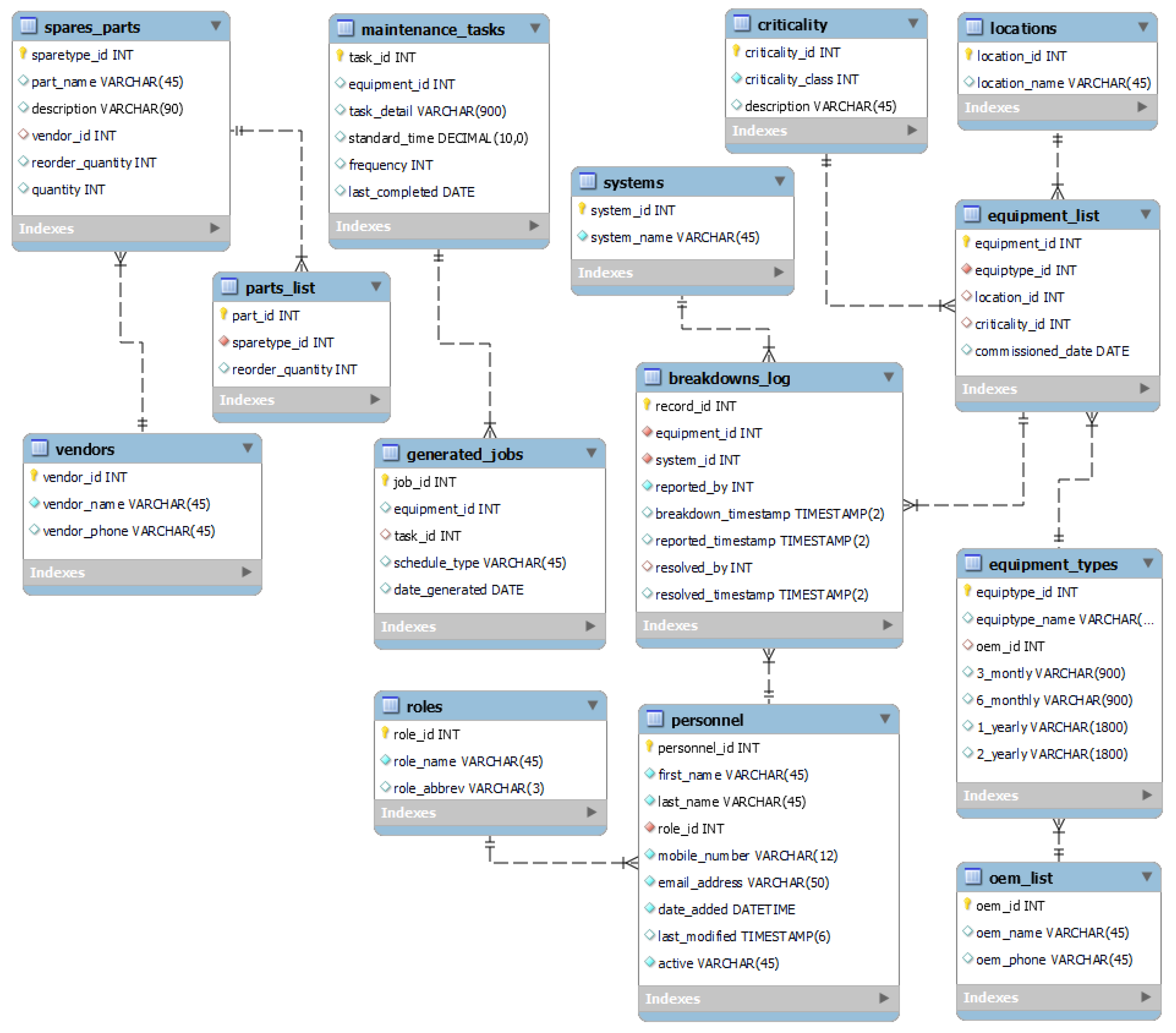
Figure 1. Hospital value chain. Adapted from [35,36].
Modelling 04 00013 g001
Figure 2. Entity relationship diagram for maintenance system’s database design in MySQL Workbench 8.0.
Modelling 04 00013 g002
Figure 3. Maintenance process flow.
Modelling 04 00013 g003
Figure 4. Maintenance system DES model. This whole model represents just the objective function in the simulated annealing model. (See also Figure 5).
Modelling 04 00013 g004
Figure 5. Logic flow showing the positioning of the DES module within the simulated annealing algorithm.
Modelling 04 00013 g005
Figure 6. Ranges of accessible solution spaces at various temperature steps.
Modelling 04 00013 g006
Figure 7. Program screenshots indicating initial and final solutions and performance summary.
Modelling 04 00013 g007
Figure 8. Initial versus final performance, maintenance tasks, durations and delays.
Modelling 04 00013 g008
Figure 9. Overall costs and inventory levels.
Modelling 04 00013 g009
Figure 10. Search history for optimal solution.
Modelling 04 00013 g010
Table 1. System variables of the healthcare maintenance DES-SA model.
Variable GroupsIndependentDependentControl
People related
-
Number of technicians, N T E C H
-
Total labour cost, C L
-
Absenteeism rate, A
-
Labour cost per technician per day, C P D
Spares related
-
Spares reorder quantity, Q O R D
-
Spares reorder level, Q L V L
-
Spares maximum level, Q M A X
-
Total spares cost, C S
-
Total spares consumed, S
-
Spares lead time, L
-
Spares cost per unit, C S U
-
Mean spares consumption per task, S T
Equipment related
-
Time between preventive schedules for asset type i, T P R E V i
-
Time between predictive schedules for asset type i, T P R E D i
-
Number of breakdowns, N B D
-
Number of preventive schedules in period, N P R E V
-
Number of predictive schedules in period, N P R E D
-
Asset availability
-
Number of asset types, n
-
Number of assets per type i, m i
-
Mean time between breakdowns for asset type i, t B D i
-
Mean time for preventive maintenance activity on asset type i, t P R E V i
-
Mean time for predictive maintenance activity on asset type i, t P R E D i
-
Mean time to repair asset type i, t R E P i
Operations related-
-
Productivity rate
-
Queue delays
-
Actual customer service level, S L A C T
-
Total unavailability cost, C U
-
Total cost, C T O T
-
Operating margin or profit, P
-
Operating time, T O P
-
Target customer service level, S L T
-
Downtime cost per asset per hour, C D T
-
Gross revenue per asset per hour, R A S T
Simulation related
-
Simulation time, t s i m
-
Initial simulation temperature, T I N I T
-
Final simulation temperature, T F I N A L
-
Cooling parameter, α
-
Metropolis probability, P r
-
Random seed, S E E D
-
Iterations per temperature step, I
Table 2. Simulation parameters and their values.
Simulation ParameterValueExplanation
-
Initial temperature
-
Final temperature
-
Cooling factor, α
Dynamic
20
0.75
-
calculated to ensure adequate acceptance probability at start, depends on asset count and other data
-
selected such that difference between successive temperatures is small enough to be no longer significant, in this case <10
-
simple geometric cooling factor that gives an adequate cooling profile
-
Iteration per temperature step
50
-
chosen to be large enough to allow for sufficient exploration of solution space, but not too high as to increase the computational expense significantly
Table 3. Set of input parameters.
Asset Group 1 2 3 4 5 6 7 8 9 10
Units per group 44365710280
MTBF [weeks] 301032923222910178
Preventive maintenance interval [weeks] 525252nevernevernevernevernevernevernever
Predictive maintenance interval [weeks] 13131313262626262613
Disclaimer/Publisher’s Note: The statements, opinions and data contained in all publications are solely those of the individual author(s) and contributor(s) and not of MDPI and/or the editor(s). MDPI and/or the editor(s) disclaim responsibility for any injury to people or property resulting from any ideas, methods, instructions or products referred to in the content.