Abstract
In recent years, bounded distributions have attracted extensive attention. At the same time, various areas involve bounded interval data, such as proportion and ratio. In this paper, we propose a new bounded model, named logistic Truncated exponential skew logistic distribution. Some basic statistical properties of the proposed distribution are studied, including moments, mean residual life function, Renyi entropy, mean deviation, order statistics, exponential family, and quantile function. The maximum likelihood method is used to estimate the unknown parameters of the proposed distribution. More importantly, the applications to three real data sets mainly from the field of engineering science prove that the logistic Truncated exponential skew logistic distribution fits better than other bounded distributions.
1. Introduction
In daily life, data related to percentage and proportion are bounded. For example, the proportion of charitable donations in income needs a bounded continuous distribution to describe it; see Papke and Wooldridge [1]. In the statistical literature, Beta distribution is a famous bounded distribution. However, its cumulative distribution function (cdf) is not a closed expression and contains special functions. Scholars have therefore proposed bounded distributions that were more flexible than the Beta distribution. Topp and Leone [2] proposed the Topp–Leone distribution, which was useful to model life cycle phenomena and was used as an alternative to Beta distribution in many respects. Pourdarvish et al. [3] studied a generalization of Topp–Leone distribution referred to as the exponentiated Topp–Leone distribution. They discussed many aspects of this new model, such hazard rate function, the moments, and the order statistics, and applied it to milk yield data. Kumaraswamy [4] introduced another widely used distribution referred to as the Kumaraswamy distribution with bounded support, which was applicable to many natural phenomena in which the process values were bounded on both sides. Lemonte et al. [5] used the exponentiated Kumaraswamy distribution for reliability and life analysis and emphasized that its advantage over Beta distribution was a simple explicit formula of distribution and quantile function without involving any special function.
In recent years, there has been increasing interest in introducing new distributions defined on bounded support. Gómez-Déniz et al. [6] described that log-Lindley distribution could be effectively applied to different scenarios, such as actuarial settings or econometric analysis. Especially in insurance, the log-Lindley regression model could be regarded as an alternative to the classical Beta regression model. Altun and Hamedani [7] claimed that the advantage of log-xgamma distribution lied in its simple form and certain flexibility through risk rate function, and it could be used to model life cycle data sets. Korkmaz [8] showed that logit slash had a good fitting effect for high-kurtosis skewness data sets with outlier observations and that the proposed model could be an alternative to the classical bounded distributions available in the statistical literature to model percentage and proportion. Mazucheli et al. [9] demonstrated that the unit-Weibull regression model was more suitable for modeling health, accounting, and social science data sets than Beta and Kumaraswamy regression models. Altun [10] discussed the flexibility of log-weighted distribution through the educational-attainment and self-reported-health data sets of OECD countries and a new regression for bounded response variable was introduced based on the log-weighted distribution.
The Truncated-exponential skew-logistic (TESL) distribution is a member of the skew logistic distribution family, which was studied by Mirzadeh and Iranmanesh [11]. Compared with other skew logistic distributions, the TESL distribution has closed expressions of the the probability density function (pdf), cdf, and quantile function. In addition, the TESL distribution belongs to the exponential family. Therefore, the skewness parameter can be derived more easily. Meanwhile, the TESL distribution can be used to model unimodal data with certain skewness. Compared with other skew logistic distributions, the TESL distribution was better than other models. A random variable Y has a TESL distribution with parameters , and , denoted by TESL, if its pdf is given by
The cdf of Y is given by
In this paper, we introduce a new bounded distribution, named by the logit TESL (LTESL) distribution, which is generated from , where Y follows the TESL distribution introduced in the literature. The new distribution has closed and tractable properties, such as its pdf, and cdf and quantile functions have explicit forms. Since the pdf of the proposed distribution is explicit and straightforward, the parameters of the new distribution can be estimated by maximum-likelihood estimation. The application results show that compared with other bounded distributions on the unit interval, the new distribution provides better modeling ability.
The rest of the paper is organized as follows: Some important mathematical properties of the new distribution are derived in Section 2, such as cdf, moment, mean residual life function, Renyi entropy, mean deviation, order statistics, exponential family, and quantile function. The maximum-likelihood estimation of the new distribution is discussed in Section 3. Simulation studies to evaluate the proposed methods are conducted in Section 4. Three real data applications are studied in Section 5. Some conclusions are given in Section 6.
2. Logit Truncated-Exponential Skew-Logistic Distribution
This section describes some basic properties of the LTESL distribution, which is defined as follows.
Definition 1.
A random variable X has the LTESL distribution with parameters , and , denoted by , if its pdf is given by
Proposition 1.
Let ; the cdf of X is given by
Proof of Proposition 1.
According to the variable substitution of the integral, we have
where and . Thus, the result is obtained. □
We point out that . Next, we give some important properties of the LTESL distribution.
Figure 1 shows the possible pdf curves of the LTESL distribution with different values of parameters. From these Figures, we can see that the LTESL distribution has the following pdf shapes: decreasing and unimodal. The LTESL distribution is a good choice to model unimodal skewness data set.
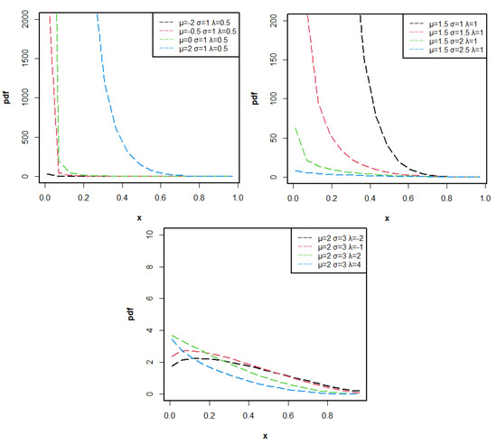
Figure 1.
The pdf curves of LTESL() for different parameters.
Proposition 2.
Let , the survival function (sf) of X is given by
the hazard rate function (hrf) of X is given by
where , and the reversed hazard rate of X is given by
Figure 2 shows some hrf curves of the LTESL distribution with different values of parameters.
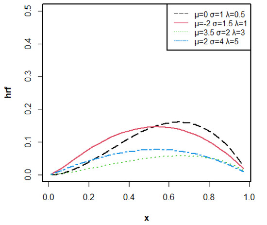
Figure 2.
The hrf curves of LTESL() for different parameters.
In mathematics and statistics, moment is a set of measures of variable distribution and morphological characteristics. For the next property, we deduce the r-order original moment of the LTESL distribution and further obtain its mean and variance.
Proposition 3.
Let ; the rth moment of X is given by
Proof of Proposition 3.
According to the definition of rth moment, we have
where is the indicator function and is probability space. Hence, the result is obtained. □
Corollary 1.
Let ; the mean and the variance of X are given by
where
and
Entropy is used to describe the degree of uncertainty of random variables. In the environment where information is represented by probability distribution, entropy represents the degree of uneven distribution of information. Renyi entropy is of great significance in statistics and social ecology.
Proposition 4.
Let , the Renyi entropy is of X, , is given by
where and .
Proof of Proposition 4.
Using the definition of Renyi entropy, we have
□
Proposition 5.
The LTESL distribution belongs to the exponential family.
Proof of Proposition 5.
Assume . Let be a function defined the same way as in Proposition 2. Then the pdf of X becomes
which means the pdf of the LTESL distribution can be rewritten as
where , , and . Therefore, the result is obtained. □
The mean residual life (MRL) function can be applied to reliability, survival analysis, economics, actuarial science, and other fields. It describes the expected survival time of an individual or object under the condition of survival at time t.
Proposition 6.
Let , the MRL function of X is given by
where .
Proof of Proposition 6.
Using the definition of MLR function, we have
Thus, the results are derived. □
Order statistics is a common and important statistic in mathematical statistics. It has a wide range of applications in the field of parametric and nonparametric statistics.
Proposition 7.
Let be a random sample coming from , and denote the corresponding order statistics. Then the pdf and cdf of the order statistic are, respectively, given by
Proof of Proposition 7.
As we all know, the pdf and cdf of are, respectively, given by
The mean deviation can be used to measure the spread of a population. In the following proposition, we derive the mean deviation of the LTESL distribution.
Proposition 8.
Let , the mean deviation about the mean of X is given by
where .
Proof of Proposition 8.
Using Equation (1) and , we have
Thus, the result is obtained. □
In regression analysis, sometimes the mean value is not a simple analytic expression. Therefore, quantile can also be used as a choice of regression model. In addition, the quantile function can also generate random numbers.
Proposition 9.
Let , the quantile function of X, , is given by
where .
Proof of Proposition 9.
For , suppose there exists a such that ; that is, . Then
Thus, the result is derived. □
3. Maximum-Likelihood Estimation
In this section, based on LTESL distribution, we consider maximum-likelihood estimation (MLE) to estimate its unknown parameters.
Let be a random sample from . The likelihood function is given by
where is the parameter vector. The log-likelihood function is given by
Therefore, the MLE , and of , and can be obtained by solving the following equations. The partial derivatives, , , and and set them to be 0, we have
Since the likelihood equation contains nonlinear functions, it is impossible to obtain the explicit form of the MLE. Therefore, numerical methods such as the Newton–Raphson method can be used to solve the above equations.
Fisher information can reflect the accuracy of parameter estimation. Therefore, we have that the Fisher information of the LTESL distribution in the following
where
4. Simulation
In this section, the MLE method is considered to estimate the unknown parameters of LTESL distribution. We carry out simulation with R software, and the simulation experiments are repeated times. In addition, we can generate random numbers from LTESL distribution according to the following steps:
- (i)
- Set , and .
- (ii)
- Simulate .
- (iii)
- Compute , then Y follows .
- (iv)
- Compute , then X follows .
The evaluation of point estimation is based on the empirical mean and the standard deviation (SD) of each sample size. We set the sample size at , and 1000, and , , and . The mean values of the parameters and the corresponding SD are shown in Table 1.

Table 1.
Parameter estimation of , , and under different samples.
From Table 1, it can be seen that as the sample size n increases, the mean value of estimators become closer to the true values and the SD decreases in all cases. In addition, the estimation is quite stable and the estimated values of all estimators tend to be more accurate.
5. Applications
In this section, we use three real data sets to verify the practicability of the LTESL distribution and compare it with some other bounded distributions, including the Beta distribution, Kumaraswamy (Kw) distribution, unit-Weibull (UW) distribution, and exponentiated Topp-Leone (ETL) distribution. The parameter estimates, minus log-likelihood, Akaike Information Criteria (AIC), Bayesian Information Criteria (BIC), and Kolmogorov–Smirnov (K-S) statistics () are listed in Table 2, Table 3 and Table 4. The of K-S is given by
where is MLE of , is the empirical distribution for the sample data, and are the ordered data defined before. Meanwhile, the AIC and BIC are defined as
where is the log-likelihood function for , k is the number of parameters of the model, and n is the size of the data set. The minimum values for AIC or BIC and maximum value for p-Value represent the best-fitted model on the data sets. Compare the LTESL distribution with the distributions defined on interval as follows.

Table 2.
The MLEs and the goodness of fit statistics for data set 1.

Table 3.
The MLEs and the goodness of fit statistics for data set 2.

Table 4.
The MLEs and the goodness-of-fit statistics for data set 3.
- (1)
- Beta distribution:where is the beta function.
- (2)
- Kw distribution:
- (3)
- UW distribution:
- (4)
- ETL distribution:
Data set 1: The first data set is related to the perforation operation on the metal plate, which has been considered by Dey et al. [12]. It represents 50 burr observations on the metal plate, for which the hole diameter is 9 mm and the sheet thickness is 2 mm. These data are related to the two different machines being compared. The data are: 0.06, 0.12, 0.14, 0.04, 0.14, 0.16, 0.08, 0.26, 0.32, 0.22, 0.16, 0.12, 0.24, 0.06, 0.02, 0.18, 0.22, 0.14, 0.22, 0.16, 0.12, 0.24, 0.06, 0.02, 0.18, 0.22, 0.14, 0.02, 0.18, 0.22, 0.14, 0.06, 0.04, 0.14, 0.22, 0.14, 0.06, 0.04, 0.16, 0.24, 0.16, 0.32, 0.18, 0.24, 0.22, 0.04, 0.14, 0.26, 0.18, 0.16.
Table 2 shows the parameter estimator results of the LTESL, Beta, Kw, UW, and ETL distributions for data set 1. The corresponding minus log-likelihood, AIC, BIC, and p-Value are also presented. As seen from Table 2, we find that the LTESL distribution has the minimum values for AIC or BIC, and maximum value for p-Value compared other bounded distributions.
Figure 3 shows the empirical distribution function for data set 1 and the estimated bounded distributions. From Figure 3, the LTESL distribution provides a qualified fit for data set 1. The distribution of sample points is roughly the same as the LTESL distribution by the Q-Q plot presented in Figure 4.
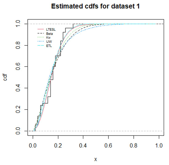
Figure 3.
Estimated cdfs for data set 1.
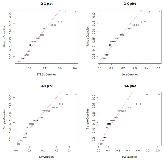
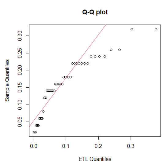
Figure 4.
Q-Q plot for data set 1.
Data set 2: The second data set covers the effective failure time of 20 components, which are taken from Nigm et al. [13]. These data are given as follows: 0.0009, 0.0040, 0.0142, 0.0221, 0.0261, 0.0418, 0.0473, 0.0834, 0.1091, 0.1252, 0.1404, 0.1498, 0.1750, 0.2031, 0.2099, 0.2168, 0.2981, 0.3465, 0.4035, 0.6143.
Table 3 shows the estimated value of the parameters, AIC, BIC, and p-value of these bounded distributions. It can be seen that LTESL distribution provides the best fit among these bounded distributions.
Figure 5 shows the fitted cdf’s of the LTESL, Beta, Kw, UW, and ETL distributions for data set 2 and suggests that the fit of the LTESL distribution is reasonable. The corresponding Q-Q plots are also displayed in Figure 6.
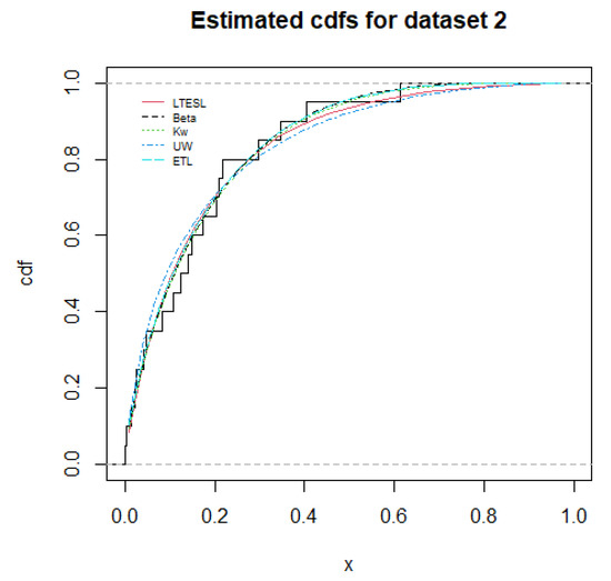
Figure 5.
Estimated cdfs for data set 2.
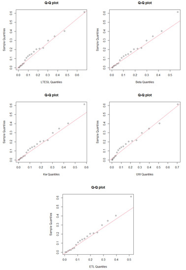
Figure 6.
Q-Q plots for data set 2.
Data set 3: The third data set considers 30 failures of an aircraft air conditioning system (in hours), which has been studied by Linhart and Zucchini [14]. This data set has recently been normalized to obtain data between 0 and 1 by Bantan et al. [15]. The data are: 0.086792453, 0.984905660, 0.328301887, 0.026415094, 0.452830189, 0.052830189, 0.233962264, 0.177358491, 0.849056604, 0.267924528, 0.928301887, 0.079245283, 0.158490566, 0.075471698, 0.018867925, 0.045283019, 0.452830189, 0.041509434, 0.011320755, 0.052830189, 0.267924528, 0.041509434, 0.052830189, 0.041509434, 0.060377358, 0.339622642, 0.003773585, 0.060377358, 0.196226415, 0.358490566.
Table 4 shows the parameter estimates, AIC, BIC, and p-Value for all fitted bounded distributions. According to Table 4, the LTESL distribution is more suitable than other bounded distributions for optimal data fitting.
Figure 7 shows the fitted models for data set 3. In Figure 7, we note that the LTESL distribution has better fitting than other bounded distributions. In addition, the corresponding Q-Q plots are also displayed in Figure 8.
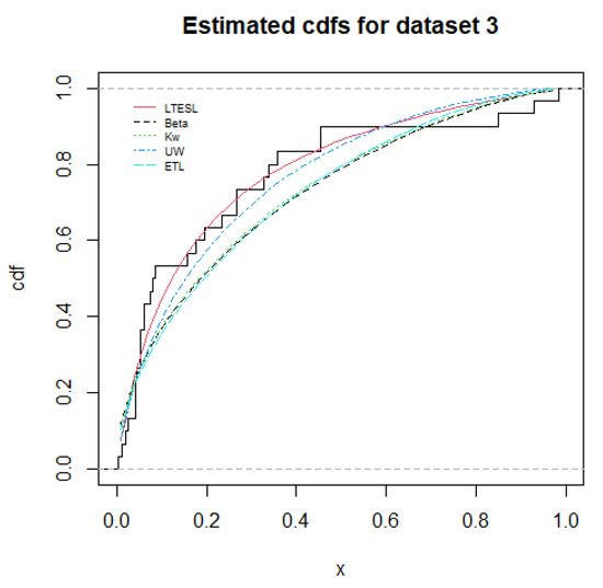
Figure 7.
Estimated cdfs for data set 3.
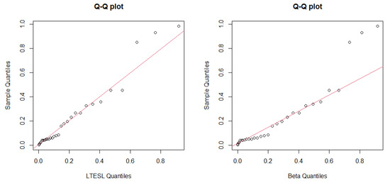
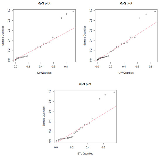
Figure 8.
Q-Q plot for data set 3.
6. Discussion
A new three-parameter LTESL distribution on bounded interval is introduced. The basic statistical properties of LTESL distribution are studied in detail, including moment, MRL function, Renyi entropy, mean deviation, order statistics, exponential family and quantile function. The maximum likelihood method for unknown parameter estimation of the proposed distribution is discussed through a simulation study. According to the analysis of real data sets in three engineering science fields, the results show that the new distribution has a better fitting than Beta, Kw, UW, and ETL distributions. Moreover, the LTESL distribution can be a good choice for processing some data in the field of engineering science.
Author Contributions
W.T.: Conceptualization, Methodology, Validation, Investigation, Resources, Supervision, Project Administration, Visualization, Writing review and editing; L.P.: Software, Formal analysis, Data curation, Writing—original draft preparation, Visualization; T.T. and X.C.: Software, Methodology, Visualization. All authors have read and agreed to the published version of the manuscript.
Funding
This research received no external funding.
Institutional Review Board Statement
Not applicable.
Informed Consent Statement
Not applicable.
Data Availability Statement
Datasets are provided in the paper.
Acknowledgments
The authors would like to thank the editor, and three anonymous referees for their careful reading of this article and for their constructive suggestions which considerably improved this article.
Conflicts of Interest
The authors declare no conflict of interest.
References
- Papke, L.E.; Wooldridge, J.M. Econometric methods for fractional response variables with an application to 401 (k) plan participation rates. J. Appl. Econom. 1996, 11, 619–632. [Google Scholar] [CrossRef] [Green Version]
- Topp, C.W.; Leone, F.C. A family of J-shaped frequency functions. J. Am. Stat. Assoc. 1955, 50, 209–219. [Google Scholar] [CrossRef]
- Pourdarvish, A.; Mirmostafaee, S.; Naderi, K. The exponentiated Topp-Leone distribution: Properties and application. J. Appl. Environ. Biol. Sci. 2015, 5, 251–256. [Google Scholar]
- Kumaraswamy, P. A generalized probability density function for double-bounded random processes. J. Hydrol. 1980, 46, 79–88. [Google Scholar] [CrossRef]
- Lemonte, A.J.; Barreto-Souza, W.; Cordeiro, G.M. The exponentiated Kumaraswamy distribution and its log-transform. Braz. J. Probab. Stat. 2013, 27, 31–53. [Google Scholar] [CrossRef]
- Gómez-Déniz, E.; Sordo, M.A.; Calder-Ojeda, E. The Log-Lindley distribution as an alternative to the beta regression model with applications in insurance. Insur. Math. Econ. 2014, 54, 49–57. [Google Scholar] [CrossRef]
- Altun, E.; Hamedani, G.G. The log-xgamma distribution with inference and application. J. Soc. Fr. Stat. 2018, 159, 40–55. [Google Scholar]
- Korkmaz, M.Ç. A new heavy-tailed distribution defined on the bounded interval: The logit slash distribution and its application. J. Appl. Stat. 2020, 47, 2097–2119. [Google Scholar] [CrossRef]
- Mazucheli, J.; Menezes, A.F.B.; Fernandes, L.B.; de Oliveira, R.P.; Ghitany, M.E. The unit-Weibull distribution as an alternative to the Kumaraswamy distribution for the modeling of quantiles conditional on covariates. J. Appl. Stat. 2020, 47, 954–974. [Google Scholar] [CrossRef]
- Altun, E. The log-weighted exponential regression model: Alternative to the beta regression model. Commun. Stat.-Theory Methods 2021, 50, 2306–2321. [Google Scholar] [CrossRef]
- Mirzadeh, S.; Iranmanesh, A. A new class of skew-logistic distribution. Math. Sci. 2019, 13, 375–385. [Google Scholar] [CrossRef] [Green Version]
- Dey, S.; Mazucheli, J.; Nadarajah, S. Kumaraswamy distribution: Different methods of estimation. Comput. Appl. Math. 2018, 37, 2094–2111. [Google Scholar] [CrossRef]
- Nigm, A.M.; Al-Hussaini, E.K.; Jaheen, Z.F. Bayesian one-sample prediction of future observations under Pareto distribution. Statistics 2003, 37, 527–536. [Google Scholar] [CrossRef]
- Linhart, H.; Zucchini, W. Model Selection; John Wiley Sons: Hoboken, NJ, USA, 1986. [Google Scholar]
- Bantan, R.A.; Chesneau, C.; Jamal, F.; Elgarhy, M.; Tahir, M.H.; Ali, A.; Zubair, M.; Anam, S. Some new facts about the unit-Rayleigh distribution with applications. Mathematics 2020, 8, 1954. [Google Scholar] [CrossRef]
Publisher’s Note: MDPI stays neutral with regard to jurisdictional claims in published maps and institutional affiliations. |
© 2021 by the authors. Licensee MDPI, Basel, Switzerland. This article is an open access article distributed under the terms and conditions of the Creative Commons Attribution (CC BY) license (https://creativecommons.org/licenses/by/4.0/).