
Parametric Model Order Reduction of Guided Ultrasonic Wave Propagation in Fiber Metal Laminates with Damage

 , ,
, ,
Abstract
:1. Introduction
2. Finite Element Analysis of Lamb Wave Propagation
3. Model Order Reduction by Proper Orthogonal Decomposition
4. Parametric Model Order Reduction
4.1. Overview
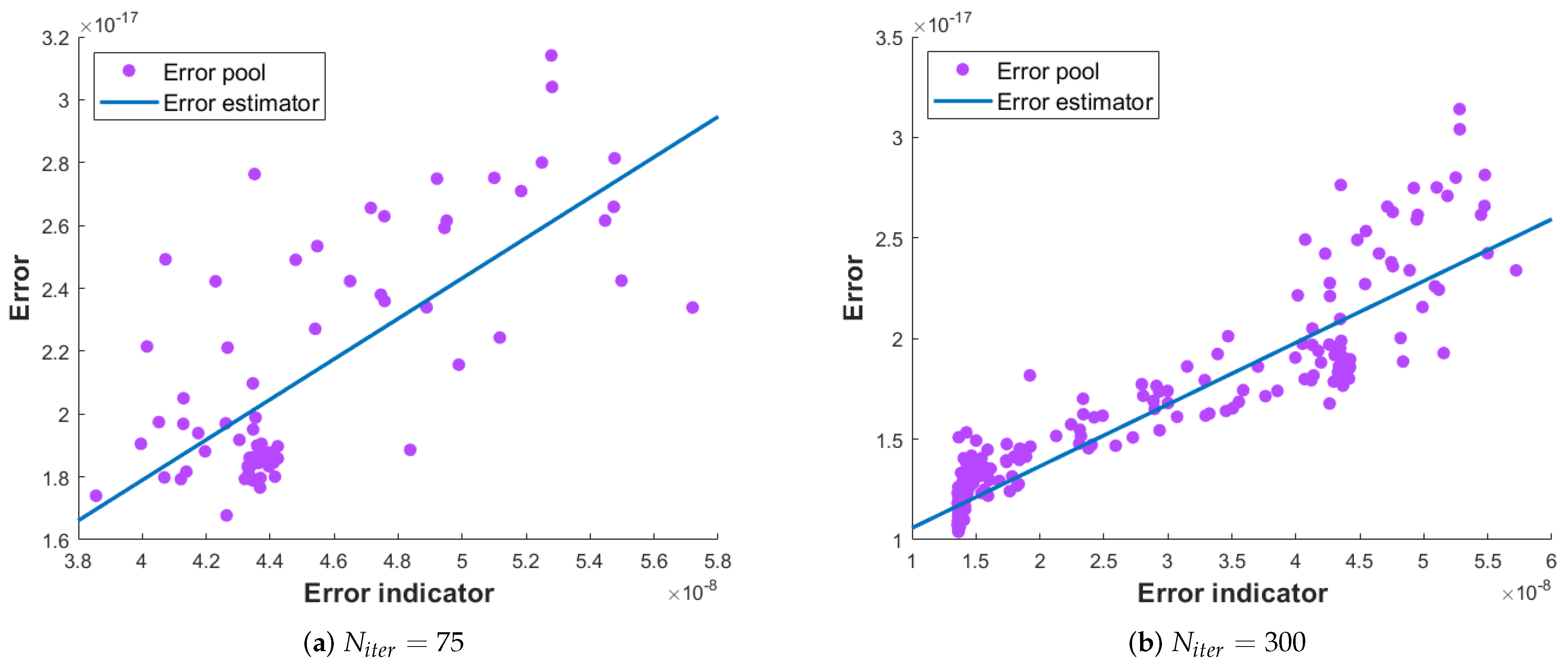
4.2. An Adaptive POD-Greedy Approach
| Algorithm 1 Identification of the additional points with maximum probability of having the highest error indicator value. |
Input: Surrogate model using multiple regression technique and its associated mean-square error Output: number of points with high probability of having largest error indicator
|
| Algorithm 2 Adaptive POD-Greedy algorithm. |
Input: Maximum number of iterations , initial cardinality of set of candidate parameters , parametric space , maximum error tolerance , Output: Global reduced-order basis
|
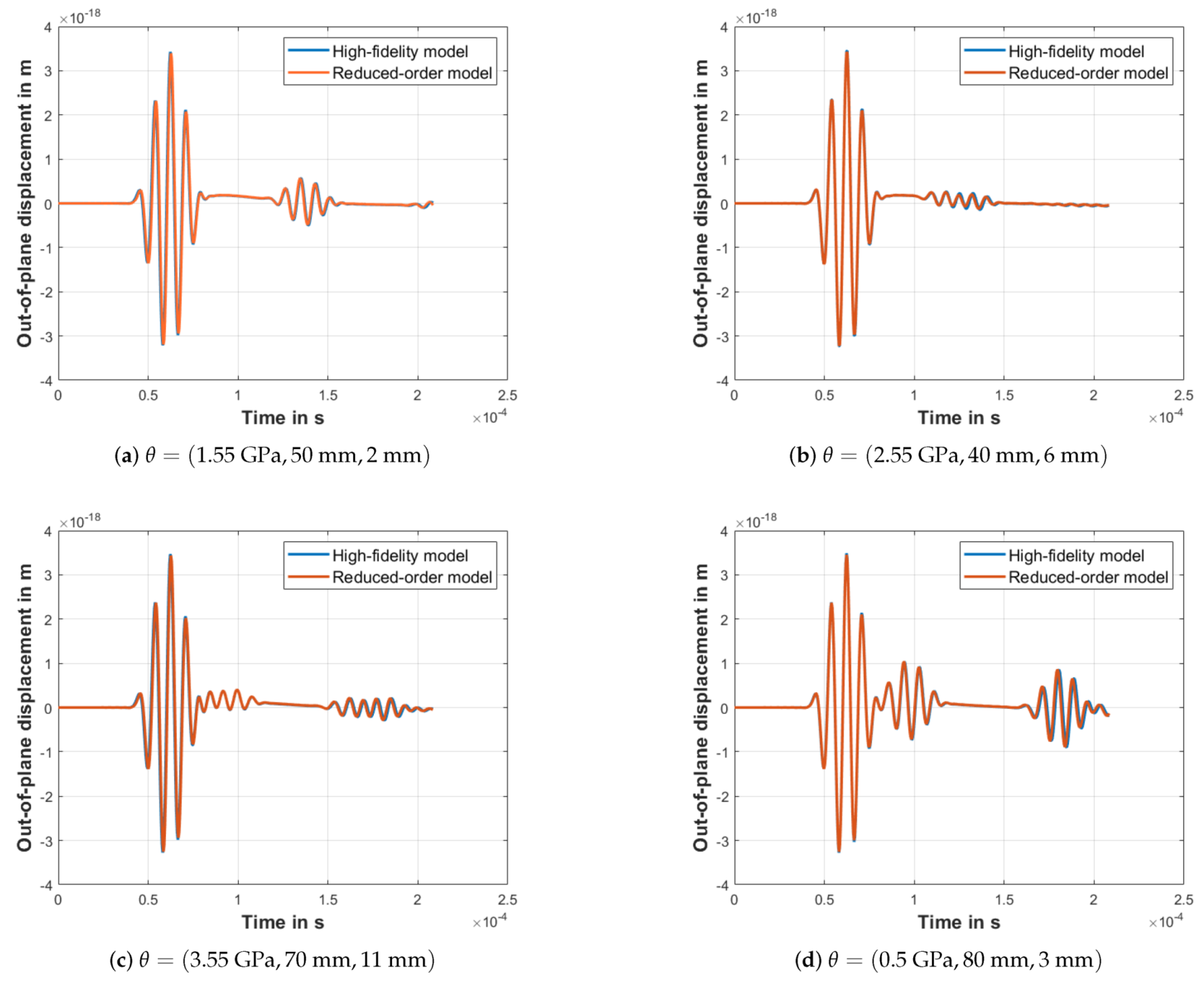
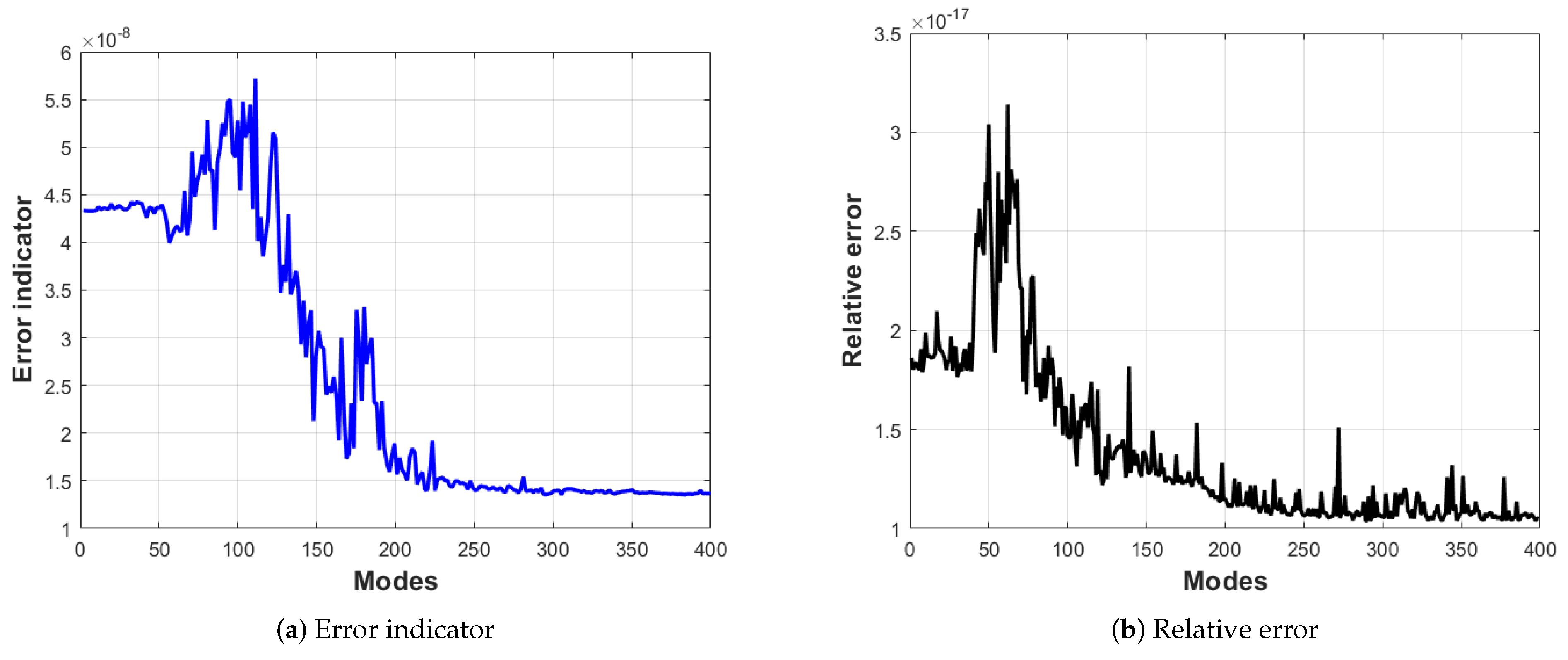
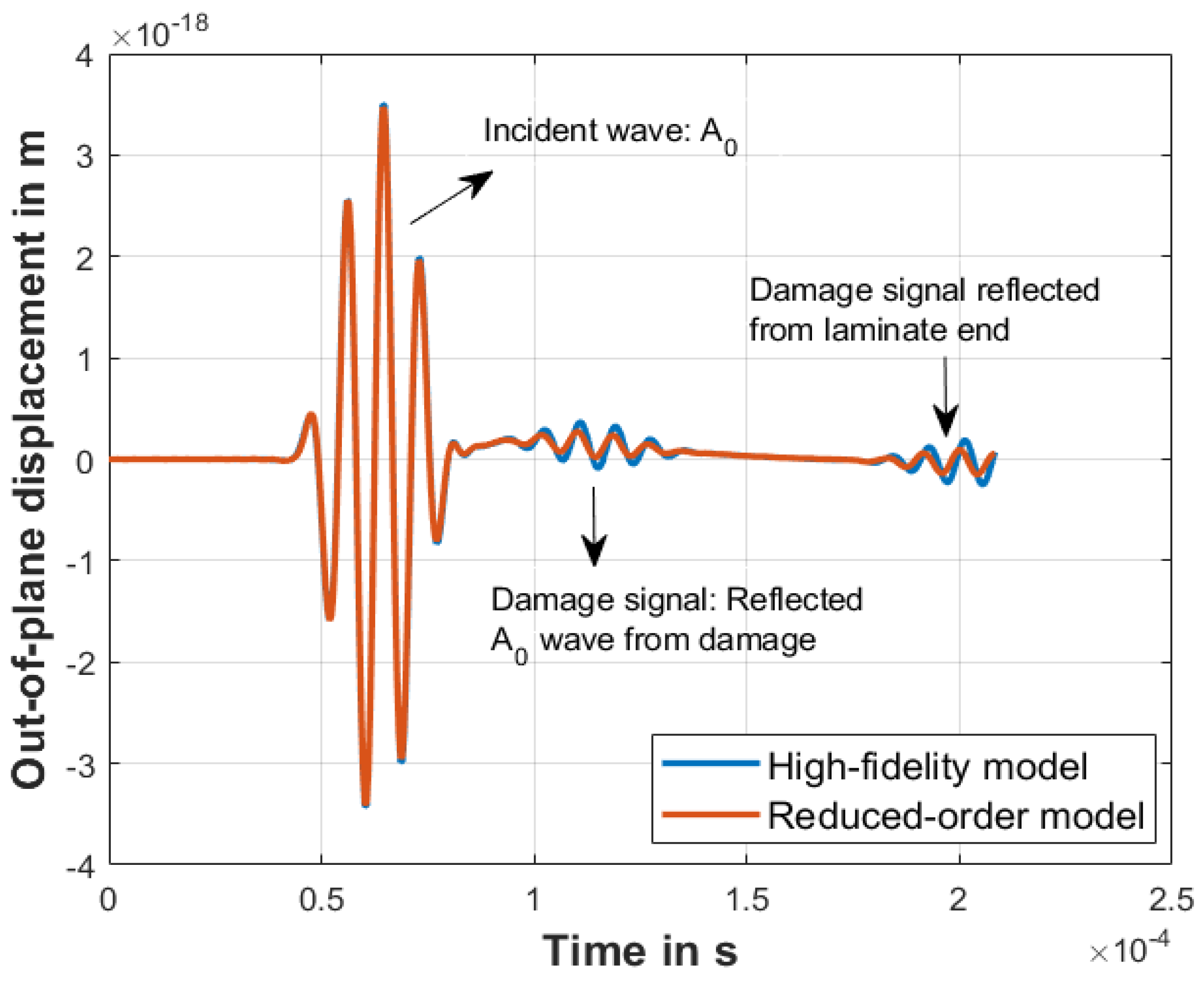
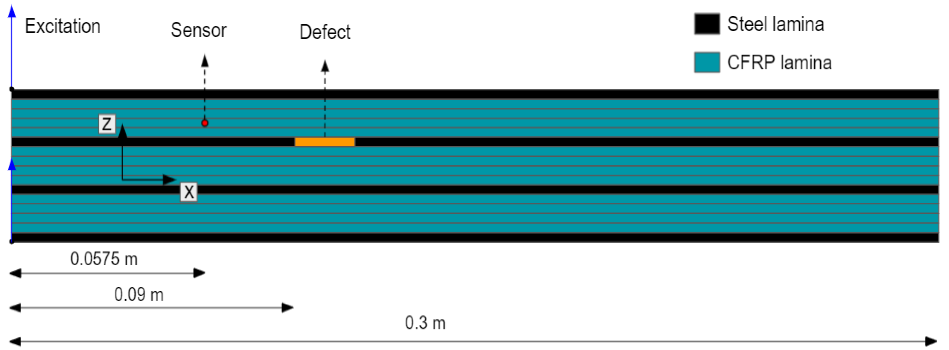
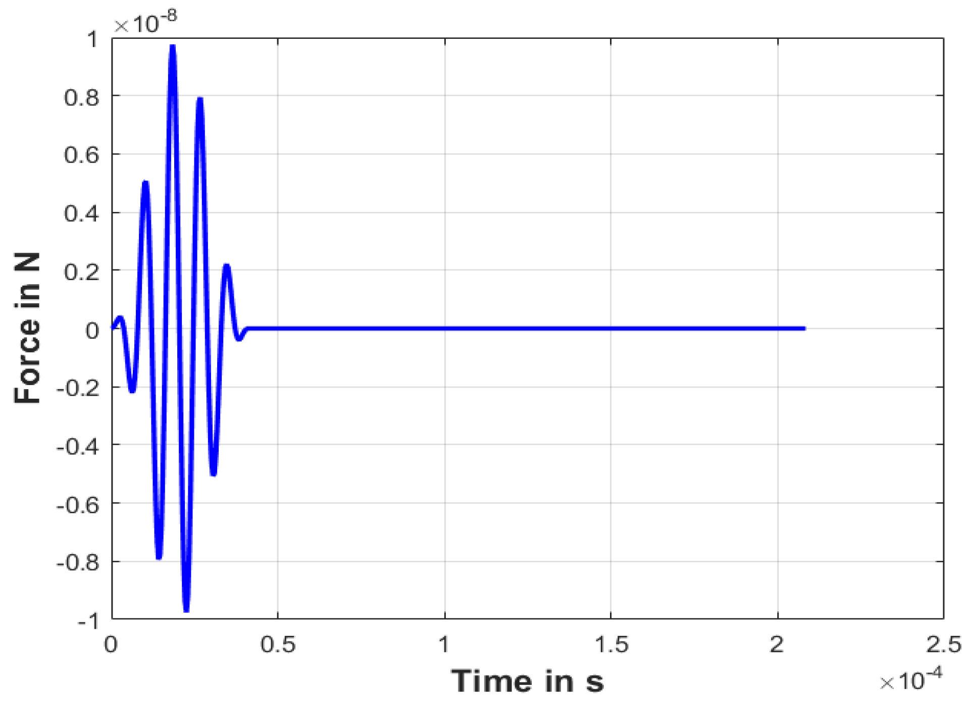
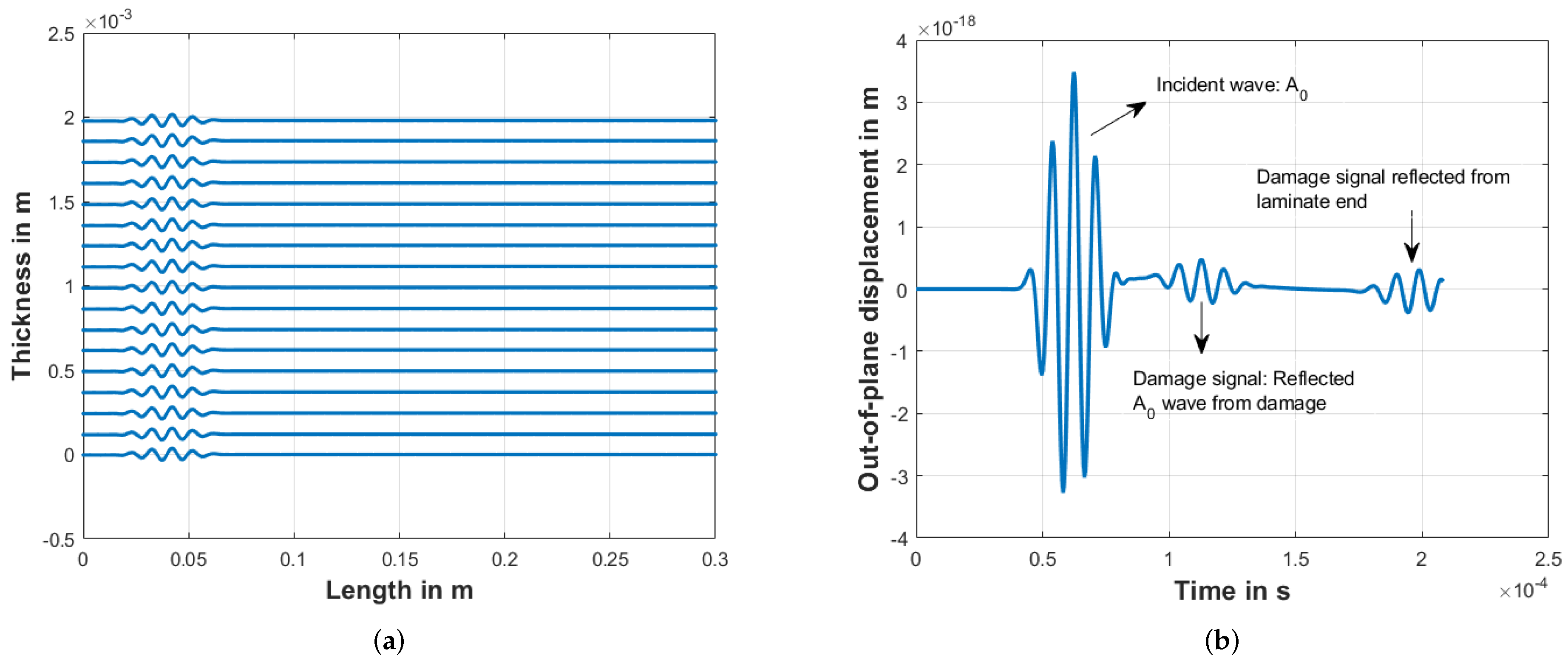
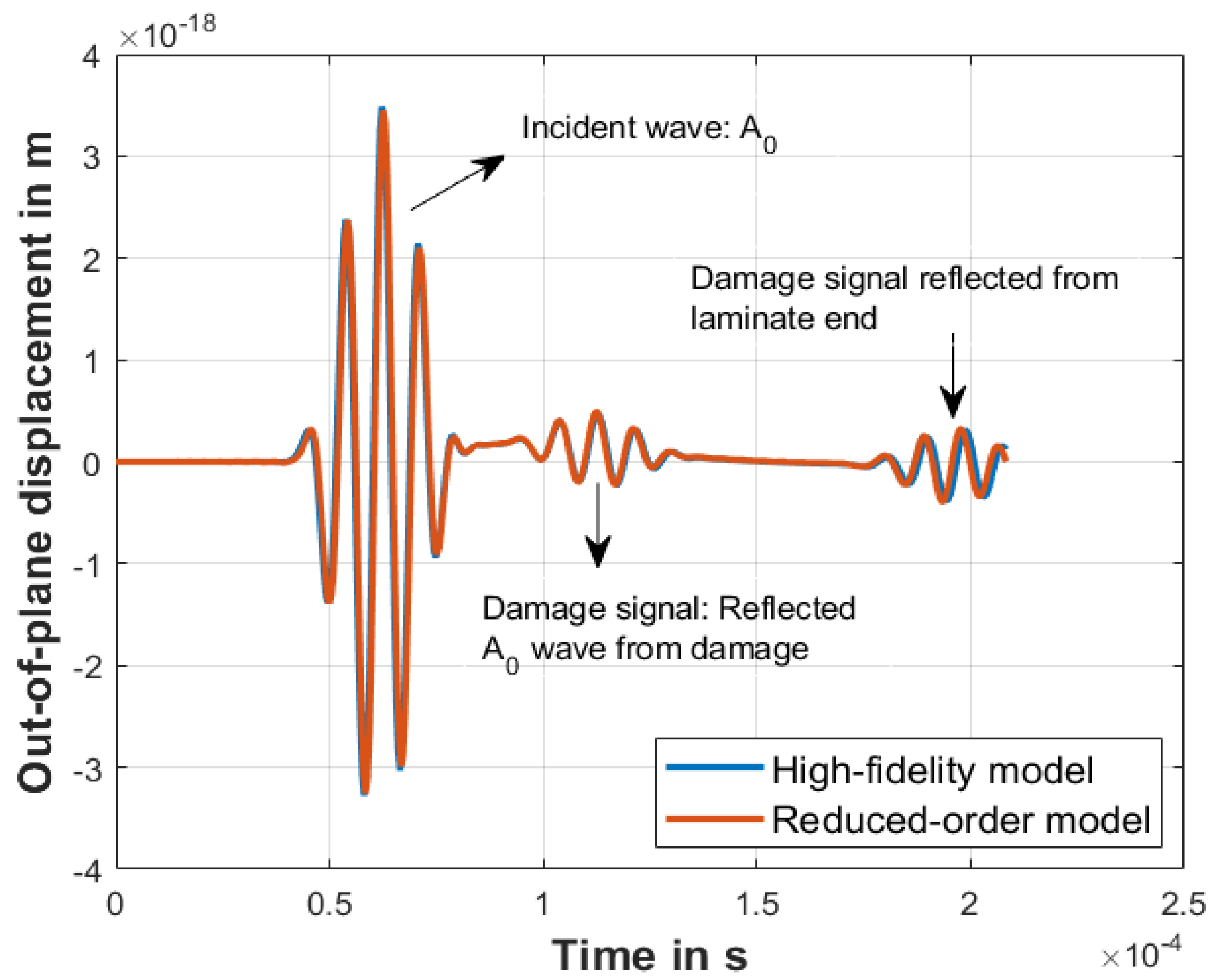
5. Application
6. Conclusions
Author Contributions
Funding
Institutional Review Board Statement
Informed Consent Statement
Data Availability Statement
Acknowledgments
Conflicts of Interest
Abbreviations
| GUW | Guided ultrasonic wave |
| FML | Fiber metal laminate |
| CFRP | Carbon fiber reinforced plastic |
| PDE | Partial differential equation |
| MOR | Model order reduction |
| PMOR | Parametric model order reduction |
| SVD | Singular value decomposition |
| POD | Proper orthogonal decomposition |
| Hi-Fi | High-fidelity model |
| CDF | Cumulative distribution function |
Appendix A. Newmark Time Integration Method
| Algorithm A1 The Newmark time integration method. |
Input: Global mass matrix , global damping matrix , global stiffness matrix , load matrix , time step size , maximum time Output: Displacement matrix at any given time instant
|
References
- Bartelds, G. Aircraft structural health monitoring, prospects for smart solutions from a European viewpoint. J. Intell. Mater. Syst. Struct. 1998, 9, 906–910. [Google Scholar] [CrossRef]
- Daniel, I.M.; Ishai, O.; Daniel, I.M.; Daniel, I. Engineering Mechanics of Composite Materials; Oxford University Press: New York, NY, USA, 2006; Volume 1994. [Google Scholar]
- Hodgkinson, J.M. Mechanical Testing of Advanced Fibre Composites; Woodhead Publishing: Sawston, UK, 2000. [Google Scholar]
- David-West, O.; Amafabia, D.; Haritos, G.; Montalvao, D. A review of structural health monitoring techniques as applied to composite structures. In Structural Durability & Health Monitoring; Tech Science Press: Henderson, NV, USA, 2017. [Google Scholar]
- Rose, J.L. A vision of ultrasonic guided wave inspection potential. In Proceedings of the 7th ASME NDE Tropical Conference-2001, San Antonio, TX, USA, 23–25 April 2001. [Google Scholar]
- Su, Z.; Ye, L.; Lu, Y. Guided Lamb waves for identification of damage in composite structures: A review. J. Sound Vib. 2006, 295, 753–780. [Google Scholar] [CrossRef]
- Guy, P.; Jayet, Y.; Goujon, L. Guided-wave interaction with complex delaminations: Application to damage detection in composite structures. In Smart Nondestructive Evaluation and Health Monitoring of Structural and Biological Systems II; International Society for Optics and Photonics: Bellingham, UK, 2003; Volume 5047, pp. 25–33. [Google Scholar]
- Ettefagh, M.M.; Akbari, H.; Asadi, K.; Abbasi, F. New structural damage-identification method using modal updating and model reduction. Proc. Inst. Mech. Eng. Part C J. Mech. Eng. Sci. 2015, 229, 1041–1059. [Google Scholar] [CrossRef]
- Glushkov, E.; Glushkova, N.; Eremin, A.; Giurgiutiu, V. Low-cost simulation of guided wave propagation in notched plate-like structures. J. Sound Vib. 2015, 352, 80–91. [Google Scholar] [CrossRef]
- Liang, Y.; Gao, X.W.; Xu, B.B.; Cui, M.; Zheng, B.J. A reduced-order modelling for real-time identification of damages in multi-layered composite materials. Inverse Probl. Sci. Eng. 2021, 29, 73–94. [Google Scholar] [CrossRef]
- Bova, W.; Lappano, E.; Catera, P.G.; Mundo, D. Development of a parametric model order reduction method for laminated composite structures. Compos. Struct. 2020, 243, 112219. [Google Scholar] [CrossRef]
- Capellari, G.; Eftekhar Azam, S.; Mariani, S. Damage detection in flexible plates through reduced-order modeling and hybrid particle-Kalman filtering. Sensors 2016, 16, 2. [Google Scholar] [CrossRef] [Green Version]
- Moser, F.; Jacobs, L.J.; Qu, J. Modeling elastic wave propagation in waveguides with the finite element method. NDT E Int. 1999, 32, 225–234. [Google Scholar] [CrossRef]
- Rauter, N.; Lammering, R.; Kühnrich, T. On the detection of fatigue damage in composites by use of second harmonic guided waves. Compos. Struct. 2016, 152, 247–258. [Google Scholar] [CrossRef]
- Antoulas, A.C. Approximation of Large-Scale Dynamical Systems; SIAM: Philadelphia, PA, USA, 2005. [Google Scholar]
- Pearson, K. LIII. On lines and planes of closest fit to systems of points in space. Lond. Edinb. Dublin Philos. Mag. J. Sci. 1901, 2, 559–572. [Google Scholar] [CrossRef] [Green Version]
- Ly, H.V.; Tran, H.T. Modeling and control of physical processes using proper orthogonal decomposition. Math. Comput. Model. 2001, 33, 223–236. [Google Scholar] [CrossRef] [Green Version]
- Kirby, M.; Sirovich, L. Application of the Karhunen-Loeve procedure for the characterization of human faces. IEEE Trans. Pattern Anal. Mach. Intell. 1990, 12, 103–108. [Google Scholar] [CrossRef] [Green Version]
- Ahlman, D.; Söderlund, F.; Jackson, J.; Kurdila, A.; Shyy, W. Proper orthogonal decomposition for time-dependent lid-driven cavity flows. Numer. Heat Transf. Part B Fundam. 2002, 42, 285–306. [Google Scholar] [CrossRef]
- Berkooz, G.; Holmes, P.; Lumley, J.L. The proper orthogonal decomposition in the analysis of turbulent flows. Annu. Rev. Fluid Mech. 1993, 25, 539–575. [Google Scholar] [CrossRef]
- Holmes, P.; Lumley, J.L.; Berkooz, G.; Rowley, C.W. Turbulence, Coherent Structures, Dynamical Systems and Symmetry; Cambridge University Press: Cambridge, UK, 2012. [Google Scholar]
- Liang, Y.; Lee, H.; Lim, S.; Lin, W.; Lee, K.; Wu, C. Proper orthogonal decomposition and its applications—Part I: Theory. J. Sound Vib. 2002, 252, 527–544. [Google Scholar] [CrossRef]
- Wu, G.; Liang, Y.; Lin, W.; Lee, H.; Lim, S. A Note on Equivalence of Proper Orthogonal Decomposition Methods; Elsevier: Amsterdam, The Netherlands, 2003. [Google Scholar]
- Kunisch, K.; Volkwein, S. Galerkin proper orthogonal decomposition methods for a general equation in fluid dynamics. SIAM J. Numer. Anal. 2002, 40, 492–515. [Google Scholar] [CrossRef]
- Bui-Thanh, T.; Willcox, K.; Ghattas, O. Parametric reduced-order models for probabilistic analysis of unsteady aerodynamic applications. AIAA J. 2008, 46, 2520–2529. [Google Scholar] [CrossRef] [Green Version]
- Veroy, K.; Patera, A. Certified real-time solution of the parametrized steady incompressible Navier–Stokes equations: Rigorous reduced-basis a posteriori error bounds. Int. J. Numer. Methods Fluids 2005, 47, 773–788. [Google Scholar] [CrossRef]
- Billaud-Friess, M.; Nouy, A. Dynamical model reduction method for solving parameter-dependent dynamical systems. SIAM J. Sci. Comput. 2017, 39, A1766–A1792. [Google Scholar] [CrossRef] [Green Version]
- Grepl, M.A.; Patera, A.T. A posteriori error bounds for reduced-basis approximations of parametrized parabolic partial differential equations. ESAIM Math. Model. Numer. Anal. 2005, 39, 157–181. [Google Scholar] [CrossRef] [Green Version]
- Rozza, G.; Huynh, D.B.P.; Patera, A.T. Reduced basis approximation and a posteriori error estimation for affinely parametrized elliptic coercive partial differential equations. Arch. Comput. Methods Eng. 2008, 15, 229–275. [Google Scholar] [CrossRef] [Green Version]
- Haasdonk, B.; Dihlmann, M.; Ohlberger, M. A training set and multiple bases generation approach for parameterized model reduction based on adaptive grids in parameter space. Math. Comput. Model. Dyn. Syst. 2011, 17, 423–442. [Google Scholar] [CrossRef]
- Choi, Y.; Boncoraglio, G.; Anderson, S.; Amsallem, D.; Farhat, C. Gradient-based constrained optimization using a database of linear reduced-order models. J. Comput. Phys. 2020, 423, 109787. [Google Scholar] [CrossRef]
- Boncoraglio, G.; Farhat, C. Active Manifold and Model-Order Reduction to Accelerate Multidisciplinary Analysis and Optimization. AIAA J. 2021, 59, 1–15. [Google Scholar] [CrossRef]
- Ullmann, S.; Rotkvic, M.; Lang, J. POD-Galerkin reduced-order modeling with adaptive finite element snapshots. J. Comput. Phys. 2016, 325, 244–258. [Google Scholar] [CrossRef] [Green Version]
- Fahl, M.; Sachs, E.W. Reduced order modelling approaches to PDE-constrained optimization based on proper orthogonal decomposition. In Large-Scale PDE-Constrained Optimization; Springer: New York, NY, USA, 2003; pp. 268–280. [Google Scholar]
- Paul-Dubois-Taine, A.; Amsallem, D. An adaptive and efficient greedy procedure for the optimal training of parametric reduced-order models. Int. J. Numer. Methods Eng. 2015, 102, 1262–1292. [Google Scholar] [CrossRef]
- Bui-Thanh, T.; Willcox, K.; Ghattas, O. Model reduction for large-scale systems with high-dimensional parametric input space. SIAM J. Sci. Comput. 2008, 30, 3270–3288. [Google Scholar] [CrossRef]
- Liu, Y.; Li, H.; Du, H.; Tong, N.; Meng, G. An adaptive sampling procedure for parametric model order reduction by matrix interpolation. J. Low Freq. Noise Vib. Act. Control 2020, 39, 821–834. [Google Scholar] [CrossRef]
- Prud’Homme, C.; Rovas, D.V.; Veroy, K.; Machiels, L.; Maday, Y.; Patera, A.T.; Turinici, G. Reliable real-time solution of parametrized partial differential equations: Reduced-basis output bound methods. J. Fluids Eng. 2002, 124, 70–80. [Google Scholar] [CrossRef]
- Veroy, K.; Rovas, D.V.; Patera, A.T. A posteriori error estimation for reduced-basis approximation of parametrized elliptic coercive partial differential equations:“convex inverse” bound conditioners. ESAIM Control. Optim. Calc. Var. 2002, 8, 1007–1028. [Google Scholar] [CrossRef] [Green Version]
- Haasdonk, B.; Ohlberger, M. Reduced basis method for finite volume approximations of parametrized linear evolution equations. ESAIM Math. Model. Numer. Anal. 2008, 42, 277–302. [Google Scholar] [CrossRef]
- Amsallem, D.; Hetmaniuk, U. A posteriori error estimators for linear reduced-order models using Krylov-based integrators. Int. J. Numer. Methods Eng. 2015, 102, 1238–1261. [Google Scholar] [CrossRef]
- Choi, Y.; Brown, P.; Arrighi, W.; Anderson, R.; Huynh, K. Space–time reduced order model for large-scale linear dynamical systems with application to boltzmann transport problems. J. Comput. Phys. 2021, 424, 109845. [Google Scholar] [CrossRef]
- McBane, S.; Choi, Y. Component-wise reduced order model lattice-type structure design. Comput. Methods Appl. Mech. Eng. 2021, 381, 113813. [Google Scholar] [CrossRef]
- Kim, Y.; Wang, K.; Choi, Y. Efficient space–time reduced order model for linear dynamical systems in Python using less than 120 lines of code. Mathematics 2021, 9, 1690. [Google Scholar] [CrossRef]
- Cagniart, N.; Crisovan, R.; Maday, Y.; Abgrall, R. Model Order Reduction for Hyperbolic Problems: A New Framework. arXiv 2017, arXiv:hal-01583224. [Google Scholar]
- Mirhoseini, M.A.; Zahr, M.J. Model reduction of convection-dominated partial differential equations via optimization-based implicit feature tracking. arXiv 2021, arXiv:2109.14694. [Google Scholar]
- Eftang, J.L.; Patera, A.T. Port reduction in parametrized component static condensation: Approximation and a posteriori error estimation. Int. J. Numer. Methods Eng. 2013, 96, 269–302. [Google Scholar] [CrossRef] [Green Version]
- Huynh, D.B.P.; Knezevic, D.J.; Patera, A.T. A static condensation reduced basis element method: Approximation and a posteriori error estimation. ESAIM Math. Model. Numer. Anal. 2013, 47, 213–251. [Google Scholar] [CrossRef] [Green Version]
- Blockmans, B.; Tamarozzi, T.; Naets, F.; Desmet, W. A nonlinear parametric model reduction method for efficient gear contact simulations. Int. J. Numer. Methods Eng. 2015, 102, 1162–1191. [Google Scholar] [CrossRef]
- Balajewicz, M.; Farhat, C. Reduction of nonlinear embedded boundary models for problems with evolving interfaces. J. Comput. Phys. 2014, 274, 489–504. [Google Scholar] [CrossRef] [Green Version]
- Galbally, D.; Fidkowski, K.; Willcox, K.; Ghattas, O. Non-linear model reduction for uncertainty quantification in large-scale inverse problems. Int. J. Numer. Methods Eng. 2010, 81, 1581–1608. [Google Scholar] [CrossRef] [Green Version]
- Chen, P.; Schwab, C. Model order reduction methods in computational uncertainty quantification. In Handbook of Uncertainty Quantification; Springer: Berlin/Heidelberg, Germany, 2016; pp. 1–53. [Google Scholar]
- Balajewicz, M.; Amsallem, D.; Farhat, C. Projection-based model reduction for contact problems. Int. J. Numer. Methods Eng. 2016, 106, 644–663. [Google Scholar] [CrossRef] [Green Version]
- Zahr, M.J.; Avery, P.; Farhat, C. A multilevel projection-based model order reduction framework for nonlinear dynamic multiscale problems in structural and solid mechanics. Int. J. Numer. Methods Eng. 2017, 112, 855–881. [Google Scholar] [CrossRef]
- Binder, A.; Jadhav, O.; Mehrmann, V. Model order reduction for parametric high dimensional models in the analysis of financial risk. arXiv 2020, arXiv:2002.11976. [Google Scholar]
- Jones, D.R. A taxonomy of global optimization methods based on response surfaces. J. Glob. Optim. 2001, 21, 345–383. [Google Scholar] [CrossRef]
- Hesthaven, J.S.; Stamm, B.; Zhang, S. Efficient greedy algorithms for high-dimensional parameter spaces with applications to empirical interpolation and reduced basis methods. ESAIM Math. Model. Numer. Anal. 2014, 48, 259–283. [Google Scholar] [CrossRef] [Green Version]
- Newmark, N.M. A method of computation for structural dynamics. J. Eng. Mech. Div. 1959, 85, 67–94. [Google Scholar] [CrossRef]


| Density | Young’s Modulus | Poisson’s Ratio |
|---|---|---|
| (kg/m) | (GPa) | |
| 7900 | 180 |
| Young’s Modulus | ||
|---|---|---|
| (GPa) | ||
| Poisson’s Ratio | ||
| (- ) | ||
| Shear Modulus | ||
| (GPa) | ||
| Model | Training Time | Computational Time |
|---|---|---|
| High-dimensional | - | 66.29 s |
| Reduced-order | 17.6 h | 1.96 s |
Publisher’s Note: MDPI stays neutral with regard to jurisdictional claims in published maps and institutional affiliations. |
© 2021 by the authors. Licensee MDPI, Basel, Switzerland. This article is an open access article distributed under the terms and conditions of the Creative Commons Attribution (CC BY) license (https://creativecommons.org/licenses/by/4.0/).
Share and Cite
Bellam Muralidhar, N.K.; Rauter, N.; Mikhaylenko, A.; Lammering, R.; Lorenz, D.A. Parametric Model Order Reduction of Guided Ultrasonic Wave Propagation in Fiber Metal Laminates with Damage. Modelling 2021, 2, 591-608. https://doi.org/10.3390/modelling2040031
Bellam Muralidhar NK, Rauter N, Mikhaylenko A, Lammering R, Lorenz DA. Parametric Model Order Reduction of Guided Ultrasonic Wave Propagation in Fiber Metal Laminates with Damage. Modelling. 2021; 2(4):591-608. https://doi.org/10.3390/modelling2040031
Chicago/Turabian StyleBellam Muralidhar, Nanda Kishore, Natalie Rauter, Andrey Mikhaylenko, Rolf Lammering, and Dirk A. Lorenz. 2021. "Parametric Model Order Reduction of Guided Ultrasonic Wave Propagation in Fiber Metal Laminates with Damage" Modelling 2, no. 4: 591-608. https://doi.org/10.3390/modelling2040031
APA StyleBellam Muralidhar, N. K., Rauter, N., Mikhaylenko, A., Lammering, R., & Lorenz, D. A. (2021). Parametric Model Order Reduction of Guided Ultrasonic Wave Propagation in Fiber Metal Laminates with Damage. Modelling, 2(4), 591-608. https://doi.org/10.3390/modelling2040031