1. Introduction
Growth in the number of vehicles and degree of urbanization mean that the annual cost of traffic jams is increasing in cities. This leads to a decreased in the quality of life among citizens through a considerable waste of time and excessive fuel consumption and air pollution in congested areas [
1]. Early analysis of congestion events and prediction of traffic volumes is a crucial step to identify traffic bottlenecks, which can be utilized to assist traffic management centers. Research on predicting the traffic data is thus essential. Such studies are valuable for planning the allocation of limited resources to highways that are most at risk for experiencing congestion and for developing an improved intelligent traffic management service [
1]. Forecasting models need historical traffic data and supporting variables that are related to traffic demand modeling. The selection of a suitable algorithm to project traffic volumes is also essential.
With the widespread use of traffic sensors and new traffic-sensor technologies, there is a copious amount of traffic data available, which has led to the age of big data in the transportation sector. As a result, transportation management is experiencing a transformation to employ data-driven methods. However, the accurate prediction of traffic flow is still challenging because of the existence of many external disturbance factors. Hence, reliable model-based or data-based traffic flow prediction methods are contentious topics in transportation research [
2]. Even slightly inaccurate capacity predictions can lead to congestion, with vast social costs in terms of travel time, fuel consumption, and environmental pollution. Hence, accurate forecasting of traffic flow during peak periods is an essential topic that attracts interest in the literature.
The literature review revealed that most studies only focus on one or two algorithms, some linear and some nonlinear. In addition, their results showed that in some cases, linear models and some nonlinear models work best. As a result, based on the literature, the relationship between the local and global variables for forecasting traffic flow can be linear or nonlinear depending on the location and the specific issues such as type of projects or the level of analysis. Therefore, the traffic volume prediction has been limited to a few algorithms, methodologies, and a selective subset of variables in each publication. As a result, there is a gap in utilizing a universal automated framework. There has not been sufficient research regarding a universal automated framework to conduct volume prediction regarding passenger vehicles. The need for such a framework for the pipeline of traffic volume forecasting is evident in the inconsistency of existing studies’ results. Such inconsistency is striking when considering elements such as algorithm or feature-selection methods.
We implemented a universal automated framework by integrating a broad data set of Florida highways from 2001 to 2017, with 59 predictors. Through a robust cross-validation method, five linear algorithms and four nonlinear algorithms were utilized in a hyperparameter optimization framework. A grid search was then implemented to identify the best modeling approach and feature-selection method for the specific data set to minimize the mean absolute percentage error (MAPE). Previous modeling attempts produced variable results when identifying the optimal prediction parameters, as they depended on the characteristics of the original case study. Instead of developing a model, we present here our universal automated framework, which generates customizable models to maximize the performance of forecasting traffic volumes.
The primary goal of this study was to establish and validate a prediction model that exceeds the limitations of existing modes of traffic estimation. A comprehensive framework was developed that can be readily generalized to new scenarios by contractors or additional users. By analyzing a traffic data set from the State of Florida, we demonstrate the accuracy of our proposed framework and its functionality for traffic volume forecasting. New users can incorporate their data and local predictors; they can follow our methods to select parameters for an optimized model of traffic volume prediction that is specific to their project.
First, the literature review section elaborates on various traffic volume forecasting methods for long-term predictions. These include econometric regressions, travel-demand modeling, and non-parametric regression modeling. Second, the pipeline of the study is presented in the methodology section. The steps consisted of data preprocessing, feature selection, model creation (including various linear and nonlinear algorithms), parameter optimization, and evaluation of the model. Finally, in the results and discussion section, the findings are discussed in depth.
2. Literature Review
Traffic flow prediction is an important issue for transport authorities and drivers. It helps in developing a robust traffic management system and effective control measures to minimize traffic congestion and improve the efficiency of the traffic network. The emergence of connected and automated vehicles could also enhance the number of trips for passenger vehicles [
3,
4,
5]. Generally, the traffic flow forecast can be classified into three types: short-term forecasting, medium-term forecasting, and long-term forecasting. Periods of 5–30 min are usually considered short-term; from 30 min to a few hours is a medium-term forecast, and a day or longer is the long-term prediction. Traffic volume forecasting is a type of long-term prediction. It employs forecasting methods such as econometric regressions, travel-demand modeling, and neural network modeling [
1].
2.1. Short-and Mid-Term Prediction Models
Since the 1980s, scholars have investigated short- and mid-term traffic flow prediction, which is useful for real-time traffic control [
2]. The Artificial Neural Network (ANN) algorithm has frequently been applied for traffic flow prediction [
6,
7], from early studies to current ones, as it can handle nonlinearity and universal approximability of unknown functions that exist in traffic behavior. Zheng et al. [
8] mixed ANNs and Bayesian inference to predict future traffic flow.
Apart from the NN methods, there are many other prediction approaches. Examples are Kalman filter [
9], time series models [
10,
11], support vector regression (SVR) [
12], k-nearest neighbor [
13], hybrid models [
14,
15], and the gradient boosting tree regression [
16]. Comprehensive information on existing models appears in [
17,
18].
2.2. Traffic Volume Prediction Models
2.2.1. Econometric Regressions
Marshment et al. [
19] investigated econometric techniques to forecast traffic for a 1–5-year horizon for the Oklahoma Turnpike Authority. They used the autoregressive integrated moving average (ARIMA) and regression modeling approaches to predict changes in traffic volumes. Bian et al. [
20] similarly employed an unobserved component model as an econometric model to predict monthly traffic volume, with several temporal aspects.
2.2.2. Travel-Demand Modeling
The travel-demand modeling method (TDM) is a typical long-term forecast approach. It employs travel characteristics and the utilization of transport services based on land-use types as well as social and economic attributes. This type of modeling is commonly performed through a four-step process of trip generation, trip distribution, mode choice, and finally trip assignment. The annual average daily traffic (AADT) can be produced from the simulation processes. An advanced type of TDM is the activity-based model [
21]. Here, the focus is an individual’s plan and schedule, which replicates actual traveler decisions. This model usually provides relatively accurate forecasts, especially for a broad range of strategies and policies [
22].
While both TDM methods have demonstrated accurate AADT estimation, they are time-consuming to generate and require a substantial data-collection resources and modeling skills. Moreover, although TDM results are useful for informing transportation planning decisions, it is challenging to derive highly detailed information to promote traffic management, control, and route guidance for highway drivers.
Khatib et al. [
23] discovered that census levels of traffic zones and the types of centroids employed for the zones could significantly impact the quality of TDM results. Mustafa [
21] emphasized that a model with small census units could provide relatively accurate estimation of AADT. Zhong and Hanson [
24] developed a method based on geographic information systems (GIS) to forecast the traffic counts. Yang et al. [
22] investigated the uncertainty of variables used in combined TDM procedures and the classic four-step model in traffic forecasting. Their aim was to determine the level of confidence of the model outputs; they also identified and treated the uncertainties from inputs and parameters separately to enhance the accuracy of the models.
Wang et al. [
25] presented a tool to estimate AADT for highways through a TDM. The principal factor of applying the TDM in their study included employing land-use data at the parcel level. They aimed to discover the estimated number of trips produced for or associated with each parcel. The trip assignment was carried utilizing free-flow travel times and the trips were then dispersed within a trip distribution gravity model at the parcel level. The results showed that the proposed model generated 52% MAPE. This result was 159% lower than the MAPE from regression models developed for the same area [
25].
2.2.3. Non-Parametric Regression (NPR)
Non-parametric regression approaches are based on data-driven models. They highlight the underlying structures without requiring an interpretation of the relations between inputs and outputs. The main purpose of these methods is to identify data clusters that possess characteristics similar to the current state for a specific interval of prediction; the same prediction is then defined from these. This procedure avoids the need to consider a forecasting equation expressed mathematically by a set of parameters, as occurs with the parametric approach [
6,
26].
The term “non-parametric” does not imply that these models lack parameters entirely. Rather, it signifies that the features and number of parameters are not fixed initially and are adjustable, with the form and number of parameters being determined by studying the data. Usually, more data are required than is the case for parametric models. The dynamic, complex, and nonlinear characteristics of traffic flow render NPR suitable for non-parametric approaches [
27].
2.2.4. Artificial Neural Networks (ANNs)
The ANN algorithm is the most widely employed model in traffic prediction due to its ability to model nonlinear and dynamic processes [
6,
7]. Even if the underlying relationships in a data set are not transparent, an ANN model generalizes accurate predictions because of its non-parametric and nonlinear features. Artificial Neural Networks are sometimes regarded as a black box: they are not straightforward to interpret because they have multiple neurons, complex structures, and nonlinear functions. Rapid variations in traffic patterns are hard to capture by linear algorithms. By contrast, ANN models can approximate any degree of complexity, without prior knowledge of problem-solving; hence, they have attracted attention and have been recognized as a suitable choice for traffic flow forecasting models [
26,
27].
Yin et al. [
28] generated a fuzzy-neural model (FNM) to forecast traffic flow in an urban network. The FNM model generated more accurate prediction results than the back-propagation neural network model. Vlahogianni et al. [
29] successfully predicted the traffic flow pattern using an optimization strategy based on genetic algorithm; their multilayered structural optimization strategy determined the most suitable ANN structure.
Ratrouta and Gazdera [
30] employed two types of ANNs and compared the results with those from the traditional parametric method of linear regression analysis to predict average daily traffic over a year. The ANN model showed better accuracy than the linear regression method for predicting daily traffic. Fu and Kelly [
1] similarly employed ANN versus log-linear and ordinary least squares (OLS) approaches to predict traffic volume. Their comparison results showed that the ANN method achieved a MAPE of 28.58%, which meant that it outperformed the log-linear model (52.49% MAPE) and OLS (66.6% MAPE).
Duraku and Ramadani [
31] developed two combined models: (1) principal component analysis and multiple linear regression (PCA-MLR) and (2) principal component analysis and radial basis function (PCA-RBF). They used both models to forecast the traffic volumes. The results indicated that the neural PCA-RBF model yielded the least errors in traffic volume forecasting [
31].
Although ANN-based forecasting models can approximate any function, especially nonlinear functions, their limitations include difficulties in interpreting the operations of the model and determining a suitable network structure. Lanaa et al. [
32] introduced an evolving spiking ANN method to obtain long-term pattern forecasts and adapt them to real-time circumstances. Maa et al. [
33] showed that post-processing the residuals of ANN by ARIMA analysis could significantly enhance the accuracy of traffic state predictions, with reductions in the mean squared error of between 8.9% and 13.4%.
2.2.5. K-Nearest Neighbor (KNN)
The KNN approach is among the well-known NPR methods. The k events of the historical database that are most similar to the current traffic situation are utilized to forecast the desired data point. Based on the distance of the nearest events to the current situation, the results are determined through a simple average or weighted average approach.
Davis and Nihan [
34] proposed a KNN approach as a possible alternative to parametric regression approaches for short-term motorway traffic forecasting. They compared KNN results to simple univariate linear time-series forecasts to demonstrate the advantage of the NPR. Smith and Demetsky [
35] similarly showed the advantage of KNN regarding robustness in forecasting the traffic volume. Their study included different data types and sizes and investigated the differences between NN and ARIMA models. Pompigna and Rupi [
36] compared the accuracy of three parametric and non-parametric prediction models, namely, a KNN regression model, a Gaussian maximum likelihood model, and a double seasonality Holt-Winters (DSHW) exponential smoothing model. They analyzed real-life data from Italian highways. The parametric DSHW model and the KNN model yielded the best results.
2.2.6. Random Forest, Decision Tree, and Support Vector Regressor
These algorithms are among the NPR models utilized for traffic volume prediction. Decision tree (DT) allows for the creation of a highly interpretable model regarding traffic data, which can be employed to determine common patterns among different traffic data points [
37,
38]. Liu and Wu [
39] suggested using random forest (RF) for traffic flow prediction models because of the model’s robustness and practicality; their work demonstrated the generalization capabilities of this model. Support vector regressor (SVR) has also been leveraged to model traffic volume and has known superior performance compared to linear models [
40].
2.3. Independent Variables and Predictors
Many studies have shown that linear regression models that use roadway characteristics and socioeconomic factors can estimate AADT with a reasonable level of error [
25,
41,
42,
43]. Several researchers have used various independent variables to predict the traffic volume for high-volume urban highways [
41,
42,
43,
44,
45,
46,
47,
48,
49]. These independent or predictor variables have included socioeconomic variables, such as population, employment, personal income, and vehicle registration, and road characteristics, namely, the number of lanes and the location type. Tennant [
50] produced a model for evaluating traffic volumes in a rural area, including certain socioeconomic variables, using land and principles of traffic generation in Kenya, a country in East Africa. Tenant’s model employed multiple regression analysis (MLR). Neveu [
51] developed several models involving elasticity parameters in MLR to anticipate traffic volumes as AADT for various road categories. The variables included in the model were population, number of households, vehicle ownership, and employment [
51].
Duddu and Pulugurtha [
52] generated a model employing statistical methods and ANN to predict AADT based on characteristics of land-use in the city of Charlottein, North Carolina. Fu and Kelly [
1] used road classes, local residential density, local working density, average road speed, distance to motorways, region types, average car-ownership ratio, and population to develop an ANN to predict the traffic count. Raja et al. [
46] developed a model using linear regression; they employed known AADTs and collected socioeconomic and spatial variables to predict the AADT. This model relied on five independent variables, including population, number of households, employment, population-to-job ratio, and access to major highways [
53].
Licheng et al. [
54] developed a traffic prediction model for one whole day using a deep neural network based on historical traffic flow data. The aim was to examine correlations between the traffic flow during a short period and the start and end times points of the period; they also examined several other contextual parameters, such as the day of the week, the weather, and the season [
54].
2.4. The Current State of Practice at Florida Department of Transportation
The Florida statewide model (FLSWM) is a comprehensive travel-demand model that was developed using the traditional four-step modeling approach. The purpose of the statewide model is to forecast the demand changes between 2020 and 2045. In this model, the primary data source is the 2010 origin-destination (OD) Survey in Florida, which was collected at the census block level. Traffic counts collected by onsite detectors between 2001 and 2015 were employed for validation and calibration purposes. Gravity models combined with discrete choice models—such as multinomial logistic regression—were utilized in the trip distribution step to determine the destination choice of travelers. Similarly, discrete choice methods were used for the modal split in two parts: the first was a long-distance mode choice, and the second was an auto occupancy or short-distance mode choice.
For the first part of the modal split, a nested logit model transferred from the Virginia Department of Transportation (VDOT) TDM was used. In contrast, for the second part, a hybrid transit abstraction methodology was transferred from the California statewide TDM. Freight transportation forecasting was performed via a separate module, named FreightSIM. Finally, in the highway assignment procedure, seven vehicle classes were assigned in the statewide model via a multi-class user equilibrium methodology.
Model outputs were evaluated by cost-benefit analysis. The overall accuracies of the model were found to be reasonable. Updates were made to FLSWM in January 2020, and certain limitations are known; they are as follows: (1) the model calibration and validation processes rely on annual historical data; monthly or daily changes are not captured; (2) although many socioeconomic parameters were utilized, some of the essential global economic factors were not considered; (3) linear or nonlinear machine learning algorithms are not considered.
Several well-structured traffic volume prediction models exist that can predict the short-term periods accurately. However, these models perform unsatisfactorily for mid- and long-term predictions. The successful implementation of the latter analyses is hindered by a lack of appropriate traffic modeling methodologies, models, and data as well as the complexity of the transportation networks system. These complex traffic patterns make it necessary to reconsider traffic count prediction by employing deep structure models with more traffic data and to consider more independent variables than in previous models. In practice, due to the various unpredictable or disruptive trends, mid- and long-term predictions may still not be sufficiently reliable. However, if executed correctly, the models could yield a level of accuracy that can be utilized for several applications [
20].
The need for a universal automated framework is evident in the literature. There is inconsistency among the previously successful approaches in terms of their algorithms, feature-selection methods, and other elements of the traffic prediction forecasting pipeline. In other words, depending on the characteristics of the investigated case in each previous study, different algorithms and different final parameters have been found to be the optimal choice. Hence, instead of focusing on optimizing yet another model for a specific case study, we wanted to develop a universal automated framework that can be used to create customized models based on a specific case of interest.
We conducted a comprehensive study to develop and compare various nonlinear and linear models that can accurately forecast the traffic volumes of interstate highways. Our work thus contributes to the current field of research. Furthermore, a pipeline containing feature selection was created and optimized to assist the training of the models. To test the model, we used the Florida Department of Transportation’s (FDOT) average daily highway traffic count for cars between 2001 and 2017; we chose Florida because of its population growth, status as an immigrant destination, logistics, critical locations, and hurricane frequency.
The results of our model could provide decision support information for transportation planners and policymakers. It could aid them in choosing where to allocate limited resources—such as money, material, laborers, and time—to expand the roads most at risk for experiencing congestion.
3. Methodology and Problem Statement
The main purpose of this research was to improve the prediction of vehicle traffic volumes by developing a highly accurate forecasting model. To accomplish this, a machine learning approach was used to analyze a broad data set of historical traffic volumes, utilizing a comprehensive set of independent variables. The key objectives were as follows:
Perform a comparative analysis of different machine learning algorithms for traffic volume prediction, with consideration given to the linear and nonlinear relationships among variables.
Examine the influence of various financial markets and the US economy on traffic patterns.
Consider how road characteristics may contribute to changes in traffic volumes.
Determine the significance of spatiotemporal predictors in altering the monthly average daily traffic (MADT).
The model pipeline in this study automatically identifies the most appropriate feature-selection method and modeling approach to reduce the MAPE. This task is accomplished through hyperparameter optimization that generates a universal automated framework. Our framework thus differs from model optimization techniques that rely on a single case study.
3.1. Dependent Variables
Data used in this study were derived from the FDOT database of historic vehicle traffic. The database encompasses traffic volumes and MADT reporting from Florida highways linked to 259 locations or co-sites.
One of the constraints of this study was that we had to utilize traffic data predictors on a monthly scale in order to match the temporal level of the independent and dependent variables (predictors and traffic volumes). Ideally, data at the hourly, daily, or weekly levels would have been utilized for higher resolution. Ultimately, the monthly predictors for six Florida interstate highways were analyzed, with a total of 52,836 data points or an average of every 5.75 miles of road.
Table 1 shows a summary of the information regarding this data set.
For this research, portable traffic monitoring sites (PTMSs) were used to record the traffic counts from 211 co-sites. Telemetered traffic monitoring sites (TTMSs) were used to collect data from the remaining 48 co-sites. Data were captured at PTMSs through loop-and-axel sensors in the road, connected directly to a nearby cabinet. By contrast, data capture by TTMSs relies on wireless internet or landlines to send information to a Transportation Statistics (TranStat) office offsite.
Figure 1 illustrates the majority coverage of Florida interstates by the 259 different co-sites.
3.2. Statistical Analysis
Table 2 summarizes the passenger vehicle (PV) directional monthly traffic volumes analyzed in this study. The term “directional” refers to the 2 different data sets, one is for the direction of south to north of the road, and the other one is for the north to south direction (N/E for North or East Bound direction on the road and S/W for South or West Bound direction on the road). Determination of the data range by statistical analysis is also shown.
3.3. Predictor Variables
To accurately predict the PV traffic volumes, we used 59 independent variables, based on the literature. These variables were separated into seven categories, namely: (1) socioeconomic, (2) temporal, (3) spatial, or (4) road characteristics, and variables related to the (5) construction market, (6) energy market, or (7) US economy. Eleven socioeconomic variables were used, including population and number of employees. Temporal variables included features such as the time and month, whereas spatial variables were related to location factors such as an interstate identifier (ID) or county name. Road characteristics were defined using variables such as the lane number or maximum speed limit. Variables related to the energy market included crude oil and electricity prices, whereas variables such as construction spending and building permits were related to the construction market. Finally, the US economy, which was the largest category, contained 27 variables. They included groups such as the gross domestic product (GDP) and Dow Jones Index (DJI). Additional information on the predictor variables appears in
Figure A1 in
Appendix A.
Figure 2 shows a comparison of the trends among some of the potential predictors of traffic volume. A distinct trend was identified in each potential indicator related to the US macroeconomic, socioeconomic, construction, and energy markets (DJI, NASDAQ Composite Index: NASDAQ, Electricity Price in FL: ELECFL, Gas Price in FL: GASPFL). It is also important to mention that the
x-axis represents the number of months beginning from January 2001 to December 2018 (204 months).
3.4. Model Development
To generate a model for traffic volume prediction, we designed a workflow that consists of (1) data preprocessing, (2) feature selection, (3) model training, (4) hyperparameter optimization, and (5) machine learning based in python [
55]. The machine learning component incorporated multiple features of the Scikit-learn library. The standardized data obtained during the preprocessing steps were further separated into three data sets for training, testing, and validation. Finally, key predictors of traffic volume were identified using a feature-selection model based on the training and validation data sets.
A summary of the workflow appears in
Figure 3. The main feature of the workflow is the loop between feature selection, modeling, and hyperparameter optimization modules. This loop automatically canvassed the variations of features and modeling approaches and produced the best-performing model with the best subset of features based on the input data set.
As shown in the flowchart in
Figure 3, feature selection was applied to the normalized and partitioned data.
where
S represents the function to decide whether a feature column is selected, in a binary fashion. The selected data is the model using linear and nonlinear modeling. At inference time, the outcome for a given datapoint is calculated as follows, where
F represents the trained model:
3.5. Data Preprocessing and Partitioning
During the first stage of data processing, each independent variable was assigned a numerical value. These values were then standardized based on a normal (0, 1) distribution to allow for regularization, before being divided into the groups training, test, and validation. For the training data set, the sample of data was used to fit the model. For the validation data set, the sample of data was used to provide an unbiased evaluation of a model fit on the training data set, while tuning model hyperparameters. The evaluation becomes increasingly biased as skill on the validation data set is incorporated into the model configuration. Ultimately, using the test data set, the data sample is used to provide an unbiased evaluation of a final model fit on the training data set.
In this study, the validation data set was mainly used to describe the evaluation of models when tuning hyperparameters and data preparation. The test data set was mainly used to describe the evaluation of a final tuned model, compared with other final models.
A nested cross-validation expanding window method was employed [
56], as illustrated in
Figure 4. This procedure was chosen to consider the integrity and temporal continuity of the time-series data set being analyzed. The training data set begins with a training subset, and a validation set is positioned within the inner loop (illustrated by the yellow and dashed boxes). This study employed a 4-fold cross-validation method (both inner and outer loop uses a 4-fold cross validation) and Each data set begins with three years’ worth of serial data, while the training set was escalated three years at every split. The three years of the data set after the validation data set were then assigned to the testing data set. As shown in
Figure 4, each split of the inner loop was implemented through a research pipeline. In the outer loop, to ensure that the final model was robust and avoided the shortcomings of an overfit or randomly acute model, any error after each split was averaged.
Table 3 shows the description of the inner and outer loops of the employed cross-validation in this study.
3.6. Performance Measurement Scales
Four different methods were appraised for measuring error in the models and the ability to gauge the proficiency of feature-selection and modeling approaches. They were the MAPE, the mean absolute error, the room mean squared error (RMSE), and R-squared. These methods were selected to include both scale-dependent (RMSE) and scale-independent (MAPE) procedures. In addition, each method provides insight regarding potential errors in forecasting, with consideration given to the traffic volume data set used in this study. These choices ensured that any error in the results could be interpreted as such. MAPE was found to be the most appropriate mean for error evaluation in this study and was subsequently used for model evaluation.
3.7. Feature Selection
In an effort to improve accuracy, feature selection was employed based on the structure of the model used in this study. This process involved filtering out any unnecessary independent variables to select only the most appropriate ones. The potential impact on precision by each variable was measured and evaluated, and low-scoring or superfluous variables were removed. If retained, unnecessary features would decrease the model’s predictive capabilities and precision.
The nested cross-validation method previously outlined was used to reinforce the training, validation, and testing of the model for each parameter set. To identify key features of the developed models, we employed the following three methods.
Bayesian ridge regression (BR), ridge regression (“ridge”), decision tree (DT), and random forest regression (RF) were utilized for implicit feature selection. We used the SelectFromModel function in Scikit-learn library [
57]. At this step, values tested for the importance threshold alternated between 0.25, 0.5, 0.75, 1, 1.25, 1.5, and 1.75 to consider the parameter selection.
To gradually pinpoint and remove superfluous features, we used the recursive feature elimination (RFE) in Scikit-learn library [
57] until only features of high importance remained. This step utilized the previous models (FRE-RF, ridge, RFE-BR, and REF-DT). The resulting numbers of selected features included 1, 3, 5, 10, 20, 30, 40, 50, and 60.
Finally, the K most appropriate data set features were identified by a scoring function, SelectKBest in Scikit-learn library [
57]. For the purpose of this study, mutual information (MFCLASSIF) and ANOVA F-value (FCLASSIF) were used. At this stage, the final number of selected features varied as before, namely 1, 3, 5, 10, 20, 30, 40, 50, and 60.
Each method was used within a grid search. Thereafter, the principle sets of selected parameters were compared.
3.8. Modeling Approaches
For the purpose of PV traffic volume forecasting, we employed several machine learning (ML) algorithms. We chose ANN, RF, DT, and KNN as nonlinear regression models using the SelectFromModel function in Scikit-learn library [
57]. For the linear models, ridge, stochastic gradient descent (SGD) regression, passive-aggressive regression (PA), linear regression (“linear”), and BR were selected. We again used the SelectionFromModel function in Scikit-learn [
57].
The selected regression models allowed for the manipulation of parametric models while also ensuring that methods with varying levels of nonlinearity or linearity could be compared. As mentioned earlier, data were split to train, validate, and test the models using a nested cross-validation approach. After this step, the ML methods were applied. For training, an expanding data window was utilized. The data from the three years after data set training were then used for validation. Finally, this process was tested on data from three additional years in sequence.
The model parameter (MP), or the highest value of the binary tree depth, varied among 5, 20, 50, 75, 100, and 200 for all RF and DT algorithms. The MP for the KNN algorithm varied among 1, 3, 5, 7, 10, and 16. In the case of ANN models, the MP alternated between 16, 64, and 256, and corresponded to the number of neurons (1 hidden layer was employed in this study). MP selection for the linear algorithm was also performed. With BR, the MP was used to illustrate the prior gamma distribution (alpha_1 and alpha_2) inverse scale parameters and shape. For ridge, the MP is indicative of the regularization strength (alpha); whereas for PA, the MP is the maximum step size (regularization C). For all three algorithms, the MP varied between 0.1, 1, 10, 100, 10,000, and 1,000,000. Finally, MP values fluctuated among 0, 0.15, 0.3, 0.5, 0.75, and 1 for SGD regression and can be attributed to the L1 ratios (L1 and L2 regularization) elastic net mixing parameter.
Table 4 presents the various models and the associated modeling parameters employed in this study.
As established in these two sections, the hyperparameter optimization grid we developed incorporated an extensive range of reasonably low to high parameter values. This allowed the model to be applied to multiple data sets containing distinctive features.
4. Results
Figure 5 shows a comparison of accuracy for the different models regarding the total PVs—that is, the total traffic volume in both directions of the road. The results were obtained from the validation data set, utilizing the grid search of this study. The RF, KNN, DT, and ANN models performed the best when trained on the training data set and tested on the validation data set. The nonlinear models showed better results than linear models. The error shown in
Figure 5 is the average of the error of the four splits of the data set depicted in
Figure 4. The average MAPE is not the mean of MAPE for all splits, but it is MAPE calculated by concatenating all predictions from different splits on the validation sets using their temporal order. This would allow a correct MAPE to be calculated even if the number of instances in each iteration differs. This is analogous to calculating the performance of one average model predicting the future outcome for multiple splits which are not overlapped and temporally ordered. (The percentage on the
y-axis on the left shows the
R-squared and on the right, presents the MAPE and MAE error).
The results of comparing the accuracy of models on the test data set using a grid search are displayed in
Figure 6. It is evident that nonlinear models outperformed the linear models. Among the nonlinear models, RF, KNN, and DT performed better than ANN. The MAPE error on the test data set offered a reliable value at 17.46%. (The percentage on the
y-axis on the left shows the
R-squared and on the right, presents the MAPE and MAE error).
4.1. Selected Model for Current Term (Without Spatial Variables)
The RF, KNN, and DT models were noted to be the best-performing, as illustrated in
Figure 5 and
Figure 6. The KNN model finds the K-nearest instances in relation to a reference instance and provides a forecasted output by averaging these instances, allowing for interpretation. However, the KNN model is limited by its dependence on the input data sets for predictions, which can produce bias. Another disadvantage is that the KNN model must search the data each time it makes a prediction; it cannot learn—although this does simplify the updating process.
In the case of the DT model, the branches were divided based on the features to construct a DT, with the leaves being the regression output. The DT model can be used to interpret the results and decision-making process; however, because sparse data at the leaves is handled during decision making, the model has the potential to overfit if too many features are used.
The RF model was capable of employing many DTs (~500) on the data used in this study by selecting data groups at random for training. This feature maintains the edges of DTs and reduces the possibility of overfitting. Hence, it was an appropriate model to use in this study for near-term and current predictions.
Figure 7 illustrates the outcome of applying the top 10 feature-selection approaches to the validation data set. The grid search process successfully selected a set of sufficient training parameters for every feature-selection method, and the data were appropriately modeled with each feature-selection method. Of note, the MAPE from the validation data set for FCLASSIF was 16.98%, the lowest of the feature-selection methods tested. (The percentage on the
y-axis on the left shows the
R-squared and on the right, presents the MAPE and MAE error).
A comparison of the accuracy of the RF model on the four splits of the performed cross-validation using the validation data set is illustrated in
Figure 8. It is apparent that split 4, covering the entire data set, achieved a lower MAPE error, with 16.35% on the validation data set (The percentage on the
y-axis on the left shows the
R-squared and on the right, presents the MAPE and MAE error).
Ground truth and the final predictions by the RF model for the validation data set are presented in
Figure 9.
Figure 10 shows the comparison of ground truth and predictions, plotted against each other. The prediction approximately mirrors the ground truth, and the points are placed around the 45 degree line.
Figure 11 depicts the model optimization for all cars on split 4 in the validation data set. The optimum feature selection and modeling approach for this case were found to be FCLASSIF and RF, respectively. To find the best selection parameter, the number of features that were selected was changed between 10 and 40. The same approach was used to optimize the RF model by alternating the maximum depth of the trees from 5 to 200. The RF model, with the depth of 75 trained on 40 selected features, had the lowest MAPE (17.23%) for the validation data set. (The percentage on the
y-axis shows the feature importance score for the variables).
Figure 12 illustrates the relative importance of the leading categories of features that were selected as the final set of independent variables from the variable pool. Road characteristic variables, with 67.09% feature importance, ranked first among the seven categories. Socioeconomic variables, with 30.33% feature importance, were ranked second.
Figure 13 shows the six features that contributed more to the models’ output than did other parameters, for all cars. Number of lanes, which represents the capacity of roadways, had the highest impact on the prediction model, with 61.11% importance. Concerning socioeconomic features, length of paved roads in lane miles had 14.24% importance, and number of licensed drivers had 10.51%; these were the next most important features for the PV prediction model. (The percentage on the
y-axis shows the feature importance score for the variables).
4.2. Selected Model for Long-Term PV Traffic Projections (without Spatial Variables)
One limitation of the RF model is that it provides only an estimation based on the given data set values. An ANN algorithm, by contrast, has distinct neuronal layers that are individually capable of nonlinear activation function. This means the RF algorithm is appropriate for near-term and current modeling, but an ANN algorithm may be more reliably generalized to long-term projections. Using an ANN algorithm, the long-term MADT can be projected because of the model’s ability to extrapolate and generate prediction values. During the model training, stochastic gradient descent was used to determine ANN bias and weights.
Cross-validation of the implementation of the ANN algorithm on the validation data set from four splits is illustrated in
Figure 14. The lowest MAPE error was a prediction accuracy of 81% for split 4. This value improved when considered with the accuracy from the additional splits. (The percentage on the
y-axis on the left shows the
R-squared and on the right, presents the MAPE and MAE error).
ANN models have various parameters that need to be optimized. To find the best selection parameter, the number of features that were ultimately selected was varied between the importance threshold of 0.25 and 1.75, using a grid search. The same approach was taken to optimize the ANN model by altering the maximum number of neurons in the hidden layer from 16 to 256. The model optimization of the total PVs on the fourth split on the validation data set for the ANN models that are illustrated in
Figure 15 showed that the DT feature-selection approach with importance threshold of 0.25 and the ANN model algorithm with 256 neurons in the hidden layer has the lowest MAPE of 18.29% on the validation data set. Moreover, the developed ANN model had an MAPE of 19.49% for the test data set on the fourth split. (The percentage on the
y-axis shows the MAPE Error for the various MP and SP of the model).
4.3. Spatial Variables
It is vital to examine the influence of spatial variables related to the location of the input data of each co-site (or “site”) in the car traffic prediction model. To test the importance of spatial variables in the model, we added four variables into the prediction model’s predictors. They are shown in
Table 5. These spatial variables studied in this study among the prior candidate variables used in the developed model in the previous section.
Comparison of the different models for performance on the test set showed that nonlinear models outperformed linear models. The MAPE error of the model with candidate spatial variables (added to the previous data set) indicated a better performance than the model without spatial variables. The comparison of the models is shown in
Table 6 and indicates a 4.31% improvement in the accuracy of the MADT by adding the spatial variables.
A comparison of the accuracy of the RF model with spatial variables for the four splits of the cross-validation is shown in
Figure 16. It is apparent that split 4 outperformed the other splits of the data. Split 4 had a MAPE error of 12.01% for the test data set.
Figure 17 depicts the optimum feature-selection and modeling approach for this case. The best models were the REFRF and RF, respectively. To find the best selection parameter, we changed the number of features that were ultimately selected between 10 and 40. The same approach was used to optimize the RF model, by altering the maximum depth of the trees from 5 to 200. The RF model with the depth of 75, trained on 40 selected features, had the lowest MAPE of 12.06% for the validation data set. (The percentage on the
y-axis shows the MAPE Error for the various MP and SP of the model).
Figure 18 shows the categorical feature importance for the best-performing models for total PVs (with spatial variables). The road characteristic category had the most significant impact on the PV traffic prediction model, at 54.78%. (The same result was evident for the previously developed model without spatial variables.) The socioeconomic category, with a value of 22.12%, was ranked second. The spatial category, with 21.62%, was third.
Figure 19 shows the six most important features that contributed to the model’s output for total PVs for the model with spatial variables. The number of lanes (which reflects the capacity of the road in the studied location) had 51.95%, indicating the most important influence on the PV prediction model. The Euclidean geometry, related to the spatial variables, achieved 14.93% and was the second most important feature (The percentage on the
y-axis shows the feature importance score for the variables).
This study also developed separate models for each direction of the traffic flow, namely north/eastbound and south/westbound. The model optimization of the north/eastbound traffic of PVs (with spatial variables) on the 4th split on the validation data set for the RF models showed that the RFERF feature-selection approach with 30 selected features, and the RF model algorithm with 75 trees had the lowest MAPE of 12.26%. The model optimization for the south/westbound traffic of PVs (with spatial variables) on the 4th split on the validation data set showed that the RFERF feature selection had the lowest MAPE, at 11.61%. It had 20 selected features and the RF model algorithm had 50 trees.
4.4. Selected Model for Long-Term PV Traffic Projections (with Spatial Variables)
The comparison of the developed ANN models is shown in
Table 7. The results confirmed a 2% improvement in the accuracy of the MADT by adding the spatial variables.
A comparison of the accuracy of the ANN model with spatial variables for the four splits of the cross-validation is shown in
Figure 20. It is apparent that split 4 outperformed the other splits of the data. Split 4 had a MAPE error of 17.48% on the test data set.
The model optimization of the total PVs (with spatial variables) on the 4th split on the validation data set for the ANN models showed that the RF feature-selection approach, with an importance threshold of 0.25, and the ANN model algorithm with 256 neurons in the hidden layer, had the lowest MAPE, at 16.79%.
Figure 21 illustrates the optimization of the developed ANN model with spatial variables.
The 4th split performed on the validation data set in model optimization for north/eastbound PV traffic was compared for each feature-selection approach used for the ANN models. The lowest MAPE score, 17.71%, was obtained for MFCLASSIF using 10 selected features and an ANN algorithm containing 64 neurons in the hidden layer. By comparison, for south/westbound PV traffic, the lowest MAPE score for ANN model optimization on the 4th split of the validation data set was 16.19%. This value was obtained by the RF feature-selection approach using an algorithm with 256 neurons in the hidden layer and 0.25 as the importance threshold. The comparison of the models with and without spatial variables on the various folds for the test and validation data set is shown in
Table 8.
5. Case Study
To test the validity of the directional ANN models (with spatial variables included) developed in this research, we used the framework to forecast directional traffic volumes between 2018 and 2050. To provide the model with input, the future values for independent variables were generated by several univariate modeling techniques. To generate time-series predictors, we used smoothing and autoregressive moving average (ARMA). The ARMA is the most commonly used classification method for univariate time-series prediction; it is represented as an average (p,q), where q corresponds to the MA order and p is equal to the AR order.
An autocorrelation correlogram function was used in addition to an autocorrelation correlogram function (PACF) to select the order of the AR and MA parameters. The smoothing method, by contrast, incorporates four aspects. These include exponential, double exponential smooth, simple, and Holt-Winters. The Holt-Winters is further defined as linear, seasonal additive, or multiplicative additive.
We selected multiple categories to classify the 59 independent variables that were used. To predict future values, ARMA and smooth methods were employed for the following categories of variables: energy market, US economy, construction market, and socioeconomic (excluding centerline miles, length of paved road line miles, population, and licensed drivers). We employed the results reported by Rayer et al. [
58] for the variables of population and licensed drivers. For the last two variables in the socioeconomic category, namely, length of paved road line miles and centerline miles, we assumed that the length of paved roads on Florida highways would remain constant over the future and for the prediction time frame. We assumed the same for spatial variables and variables for road characteristics.
To illustrate the results of the 2018–2050 projection using the direction ANN model outlined with the projected independent variables, two different co-sites were chosen from interstate highways I4 and I10. The case studies are described below.
Case Study 1: I4, Orange County, Co-site ID: 750668
Figure 22 shows the total historical and projected PV traffic employing the directional ANN model (with spatial variables) developed by the framework of this study. The historical traffic data spanned 2001 to 2017, from month 1 to month 204, reflecting the MADT of PVs. The projected values pertain to the MADT from 2018 (beginning month 205) to 2050 (ending month 600).
Case Study 2: I10, Duval County, Co-site ID: 720832
Figure 23 illustrates the total historical and projected PV traffic for case study 2. The directional ANN model with spatial variables was used.
6. Discussion
As demonstrated, the proposed framework showed high accuracy in its predictions. The framework can be used as a complementary tool for analyzing existing models of traffic volume prediction. The results of this study showed that nonlinear models had an advantage over linear models, as evident in the different performance regarding the traffic data set we used.
A universal framework developed by Mahdavian et al. [
59] followed the same pipeline generation as our study but used a data set that included 20 years of highway construction costs in Florida, unlike the traffic data structure in our study. Considering our results as well as those earlier ones, the pipeline performs adequately and the framework has sufficient generalizability, as it has been successful in both studies.
Previous studies showed that linear regression models utilizing roadway characteristics and socioeconomic factors could predict AADT with a reasonable level of errors [
25,
41,
42,
43]. However, this study has demonstrated that even when using a broader category of predictors, linear models were unable to predict the traffic count with reasonable (with actual and estimated variables matching closely) accuracy for the data set we used. In addition, our work confirms the results obtained by Liu and Wu [
39], indicating that the RF algorithm can predict traffic flow with high accuracy due to the fact of its robustness and practicality, although only for short-term predictions.
Additionally, the RF and ANN models developed by the framework of our study showed better accuracy than the TDM model developed by Wang et al. [
25], who reported a 52% MAPE. Our ANN model achieved a MAPE of 17.48%, which also indicates higher accuracy than the ANN model developed by Fu and Kelly (2017), who reported a MAPE of 28.58%. Finally, our results confirm those of Ratrouta and Gazdera [
30] and Chen et al. [
27] that ANN models were more accurate than the linear regression method for predicting daily traffic.
The results of this study showed that the RF algorithm outperformed the other nonlinear algorithms for the test data set to predict the current pattern of PV traffic on highways. The generalization capacities of RF give it an advantage for current MADT projections. The developed RF model (with spatial variables) used with the test data set was able to forecast the MADT with 88% accuracy. The road characteristics category had the most substantial impact on the PV traffic prediction model, at 54.78%, and was also ranked first in the previously developed model without spatial variables. The socioeconomic category, with a value of 22.12%, had the second rank. The spatial category, with 21.62%, had the third rank.
Regarding the critical features of the RF model (with spatial variables), road characteristics played a key role, with 54.78% importance. Socioeconomic variables (22.12%) had the second most important role in PV volume prediction. The spatial category (21.62%) ranked third. The number of lanes, at 51.95%, had the strongest influence in the PV prediction model. Euclidean geometry, related to the spatial variables, was the second most important feature (14.93%). These two variables were the main ones affecting the PV traffic volumes.
The results showed that the ANN model outperformed other linear and nonlinear algorithms for the long-term prediction, with 81% prediction accuracy. Adding the spatially related variables to the developed model resulted in an increase in the accuracy to 83%.
7. Conclusions
Passenger vehicle traffic patterns and their complexity justifies the need to employ deep structure models with more data and predictions than those used in previous studies. Additionally, unpredictable and disruptive trends—such as urbanization and economic growth—mean that long-term projections might not be reliable for practical use by transportation planners. However, if executed precisely, such predictions can be accurate enough to be useful for various applications.
A review of the literature indicated that most studies have relied on only one or two linear or nonlinear algorithms. Depending on the individual case, the conclusions drawn in such studies have varied regarding the comparison of—or contrast between—linear and nonlinear models. This is to be expected because factors such as the location, project type, and level of analysis can impact the associations between local and global variables used to predict traffic volumes. A model based on input data characteristics that are universal and generalizable would thus provide benefit in optimizing the prediction of traffic volume.
To create such a framework, we utilized a broad data set of values and characteristics that incorporated all the feature-selection and modeling approaches identified in the literature. Regardless of project type, location, or the scope of a study, new users can apply this process to their data to determine the best feature-selection and modeling parameters to select components that are vital factors in traffic volume forecasting. Compared with other models, the proposed framework has multiple advantages. It not only includes all the approaches implemented in the reviewed literature but goes beyond them in terms of the number and complexity of its algorithms and feature-selection methods.
The framework we developed both eliminates several unnecessary assumptions and avoids inconsistencies in the steps of sequential methods and multiple factors and adjustments. Furthermore, much of the process has been automated, resulting in a decrease in the time and expertise needed for forecast analysis. Finally, our model improves the predictions of future traffic networks by expanding the number of predictors, thus increasing the complexity.
In conclusion, estimating the current traffic level and forecasting typical fluctuations in the MADT is necessary for many fields of transportation analysis and practice. We developed a framework that provides a valuable and viable ready-to-use method for transportation planners for PV traffic prediction. In our Florida case study, the output of the framework was an RF model to predict the current and near-term traffic and an ANN model to forecast the long-term PV traffic count. The framework demonstrated a sound balance between forecasting accuracy and ease of use. This study also illustrated the importance of including appropriate spatial variable as predictors, besides the employed pool of candidate variables.
The model’s output, namely, the predicted traffic flow, can assist planners in estimating the PV volume and levels of service from the existing traffic capacity values and by calculating the volume-to-capacity ratio (V/C) ratio for state roadways. These estimates can help with long-term planning solutions. Transportation planners could plan for the critical links on US roads that experience overcapacity issues. Furthermore, they could examine optimized solutions to enhance the traffic network well in advance.
The main shortcomings of this research include the sample size, with 259 co-sites and 17 years’ worth of historical PV traffic counts. The type of data we used was the month-level historical traffic data, whereas it might be better to use weekly, daily, or hourly data. Ultimately, to enhance the accuracy of the proposed model, the next step would be to include trends regarding the environment, energy, and politics as independent variables (predictors) in the pool of candidate variables.
For future work, it is essential to investigate the impact of automated and connected electric and shared vehicles on the traffic flow and capacity of the network. Researchers could also study the outliers in the input data set to find the underlying reasons for the remaining error. Finally, managed and express lanes have recently been explored as a traffic congestion solution, and it would be helpful to analyze their precise influence on the traffic network.
Author Contributions
Conceptualization, A.M., A.S., and A.O.; methodology, A.M., A.S., and A.O.; software, A.M. and M.S.; validation, A.M., M.S., and A.S.; formal analysis, A.M., A.S., A.O., H.L., and J.-S.Y.; investigation, A.M., A.S., H.L., and J.-S.Y.; resources, A.M., H.L., and A.S.; data curation, A.M., H.L., and M.S.; writing—original draft preparation, A.M., A.S., H.L., M.S., and A.O.; writing—review and editing, A.M., A.S., H.L., J.-S.Y., and A.O.; visualization, A.M., A.S., and M.S.; supervision, A.M., A.S., and A.O.; project administration, A.M., A.O., and A.S. All authors have read and agreed to the published version of the manuscript.
Funding
This research received no external funding.
Institutional Review Board Statement
Not applicable.
Informed Consent Statement
Not applicable.
Data Availability Statement
The data presented in this study are available on request from the corresponding author.
Conflicts of Interest
The authors declare no conflict of interest.
Appendix A. Independent Variables (Predictors)
Figure A1.
Independent variables employed in this research.
Figure A1.
Independent variables employed in this research.
Figure A2.
Independent variables employed in this research.
Figure A2.
Independent variables employed in this research.
References
- Fu, M.; Kelly, J.A.; Clinch, J.P. Estimating Annual Average Daily Traffic and Transport Emissions for a National Road Network: A Bottom-up Methodology for Both Nationally-Aggregated and Spatially-Disaggregated Results. J. Transp. Geogr. 2017, 58, 186–195. [Google Scholar] [CrossRef]
- Okutani, I.; Stephanedes, Y.J. Dynamic prediction of traffic volume through kalman filtering theory. Transp. Res. Part B Methodol. 1984, 18, 1–11. [Google Scholar] [CrossRef]
- Mahdavian, A.; Shojaei, A.; Oloufa, A. Assessing the long-and mid-term effects of connected and automated vehicles on highways’ traffic flow and capacity. In Proceedings of the International Conference on Sustainable Infrastructure 2019: Leading Resilient Communities through the 21st Century, Los Angeles, CA, USA, 6–9 November 2019; American Society of Civil Engineers: Reston, VA, USA, 2019. [Google Scholar]
- Mahdavian, A.; Shojaei, A.; Mccormick, S.; Papandreou, T.; Eluru, N.; Oloufa, A.A. Drivers and Barriers to Implementation of Connected, Automated, Shared, and Electric Vehicles: An Agenda for Future Research. IEEE Access 2021, 9, 22195–22213. [Google Scholar] [CrossRef]
- Mahdavian, A.; Shojaei, A.; Oloufa, A. Service Level Evaluation of Florida’s Highways Considering the Impact of Autonomous Vehicles. In Proceedings of the International Symposium on Automation and Robotics in Construction; IAARC Publications: Oulub, Finland, 2019; Volume 36. [Google Scholar]
- Shojaei, A.; Mahdavian, A. Revisiting Systems and Applications of Artificial Neural Networks in Construction Engineering and Managements. In Proceedings of the International Structural Engineering and Construction, Chicago, IL, USA, 20–25 May 2019. [Google Scholar]
- Mahdavian, A.; Shojaei, A.; Salem, M.; Laman, H.; Eluru, N.; Oloufa, A. A Universal Automated Data-Driven Modeling Framework for Truck Traffic Volume Prediction. IEEE Access 2021, 9, 105341–105356. [Google Scholar] [CrossRef]
- Zheng, W.; Lee, D.H.; Shi, Q. Short-term freeway traffic flow prediction: Bayesian combined neural network approach. J. Transp. Eng. 2006, 132, 114–121. [Google Scholar] [CrossRef] [Green Version]
- Guo, J.; Huang, W.; Williams, B.M. Adaptive kalman filter approach for stochastic short-term traffic flow rate prediction and uncertainty quantification. Transp. Res. Part C Emerg. Technol. 2014, 43, 50–64. [Google Scholar] [CrossRef]
- Kumar, S.V.; Vanajakshi, L. Short-term traffic flow prediction using seasonal arima model with limited input data. Eur. Transp. Res. Rev. 2015, 7, 1–9. [Google Scholar] [CrossRef] [Green Version]
- Sun, H.; Liu, H.; Xiao, H.; He, R.; Ran, B. Use of local linear regression model for short-term traffic forecasting. Transp. Res. Rec. J. Transp. Res. Board 2003, 1836, 143–150. [Google Scholar] [CrossRef]
- Wang, J.; Shi, Q. Short-term traffic speed forecasting hybrid model based on chaos-wavelet analysis-support vector machine theory. Transp. Res. Part C Emerg. Technol. 2013, 27, 219–232. [Google Scholar] [CrossRef]
- Wu, Y.; Tan, H.; Peter, J.; Shen, B.; Ran, B. Short-term traffic flow prediction based on multilinear analysis and k-nearest neighbor regression. In Proceedings of the 15th COTA International Conference of Transportation Professionals, Beijing, China, 24–27 July 2015. [Google Scholar]
- Lopez-Garcia, P.; Onieva, E.; Osaba, E.; Masegosa, A.D.; Perallos, A. A hybrid method for short-term traffic congestion forecasting using genetic algorithms and cross entropy. IEEE Trans. Intell. Transp. Syst. 2016, 17, 557–569. [Google Scholar] [CrossRef] [Green Version]
- Allström, A.; Ekström, J.; Gundlegård, D.; Ringdahl, R.; Rydergren, C.; Bayen, A.M.; Patire, A.D. Hybrid approach for short-term traffic state and travel time prediction on highways. Transp. Res. Rec. 2016, 2554, 60–68. [Google Scholar] [CrossRef] [Green Version]
- Zhang, Y.; Haghani, A. A gradient boosting method to improve travel time prediction. Transp. Res. Part C Emerg. Technol. 2015, 58, 308–324. [Google Scholar] [CrossRef]
- Vlahogianni, E.I.; Karlaftis, M.G.; Golias, J.C. Short-term traffic forecasting: Where we are and where were going. Transp. Res. Part C Emerg. Technol. 2014, 43, 3–19. [Google Scholar] [CrossRef]
- Lippi, M.; Bertini, M.; Frasconi, P. Short-term traffic flow forecasting: An experimental comparison of time-series analysis and supervised learning. IEEE Trans. Intell. Transp. Syst. 2013, 14, 871–882. [Google Scholar] [CrossRef]
- Marshment, R.S.; Dauffenbach, R.C.; Penn, D.A. Short-range intercity traffic forecasting using econometric techniques. ITE J. 1996, 37–45. [Google Scholar]
- Bian, Z.; Zhang, Z.; Liu, X.; Qin, X. Unobserved Component Model for Predicting Monthly Traffic Volume. J. Transp. Eng. Part A Syst. 2019, 145, 4019052. [Google Scholar] [CrossRef]
- Mustafa, R. Applying High-Fidelity Travel Demand Model for Improved Networkwide Traffic Estimation: New Brunswick Case-Study. In Proceedings of the 2010 Annual Conference of the Transportation Association of Canada, Halifax, NS, Canada, 26–29 September 2010. [Google Scholar]
- Yang, C.; Chen, A.; Xu, X.; Wong, S.C. Sensitivity-based uncertainty analysis of a combined travel demand model. Transp. Res. Part B Methodol. 2013, 57, 225–244. [Google Scholar] [CrossRef] [Green Version]
- Khatib, Z.; Chang, K.; Ou, Y. Impacts of analysis zone structures on modeled statewide traffic. J. Transp. Eng. 2001, 127, 31–38. [Google Scholar] [CrossRef]
- Zhong, M.; Hanson, B.L. GIS-based Travel Demand Modeling for Estimating Traffic on Low-Class Roads. In Proceedings of the 87th Transportation Research Board Annual Meeting, Washington, DC, USA, 13–17 January 2008. [Google Scholar]
- Wang, T.; Gan, A.; Alluri, P. Estimating annual average daily traffic for local roads for highway safety analysis. Transp. Res. Rec. J. Transp. Res. Board 2013, 2398, 60–66. [Google Scholar] [CrossRef] [Green Version]
- Kirby, H.R.; Watson, S.M.; Dougherty, M.S. Should we use neural networks or statistical models for short-term motorway traffic forecasting? Int. J. Forecast. 1997, 13, 43–50. [Google Scholar] [CrossRef]
- Chen, H.; Grant-Muller, S.; Mussone, L.; Montgomery, F. A study of hybrid neural network approaches and the effects of missing data on traffic forecasting. Neural Comput. Appl. 2001, 10, 277–286. [Google Scholar] [CrossRef]
- Yin, H.; Wong, S.C.; Xu, J.; Wong, C.K. Urban traffic flow prediction using a fuzzy-neural approach. Transp. Res. Part C Emerg. Technol. 2002, 10, 85–98. [Google Scholar] [CrossRef]
- Vlahogianni, E.I.; Karlaftis, M.G.; Golias, J.C. Optimized and meta-optimized neural networks for short-term traffic flow prediction: A genetic approach. Transp. Res. Part C Emerg. Technol. 2005, 13, 211–234. [Google Scholar] [CrossRef]
- Ratrouta, N.T.; Gazdera, U. Factors affecting performance of parametric and non-parametric: Models for daily traffic forecasting. In Proceedings of the 5th International Conference on Ambient Systems, Networks and Technologies, Hasselt, Belgium, 2–5 June 2014. [Google Scholar]
- Duraku, R.; Ramadani, R. Development of Traffic Volume Forecasting Using Multiple Regression Analysis and Artificial Neural Network. Civ. Eng. J. 2019, 5, 1698–1713. [Google Scholar] [CrossRef]
- Lañaa, I.; Loboa, J.L.; Capeccid, E.; Del Sera, J.; Kasabovd, N. Adaptive long-term traffic state estimation with evolving spiking neural networks. Transp. Res. Part C Emerg. Technol. 2019, 101, 126–144. [Google Scholar] [CrossRef]
- Maa, T.; Antonioua, C.; Toledob, T. Hybrid machine learning algorithm and statistical time series model for network-wide traffic forecast. Transp. Res. Part C Emerg. Technol. 2020, 111, 352–372. [Google Scholar] [CrossRef]
- Davis, G.A.; Nihan, N.L. Nonparametric regression and short-term freeway traffic forecasting. In Proceedings of the 1st Conference on Application of Advanced Technologies in Transportation Engineering, San Diego, CA, USA, 1 March 1989. [Google Scholar]
- Smith, B.L.; Demetsky, M.J. Traffic flow forecasting: Comparison of modelling approaches. J. Transp. Eng. 1997, 123, 261–266. [Google Scholar] [CrossRef]
- Pompigna, A.; Rupi, F. Comparing practice-ready forecast models for weekly and monthly fluctuations of average daily traffic and enhancing accuracy by weighting methods. J. Traffic Transp. Eng. Engl. Ed. 2018, 5, 239–253. [Google Scholar] [CrossRef]
- Alajali, W.; Zhou, W.; Wen, S.; Wang, Y. Intersection Traffic Prediction Using Decision Tree Models. Symmetry 2018, 10, 386. [Google Scholar] [CrossRef] [Green Version]
- Crosby, H.; Davis, P.; Jarvis, S.A. Spatially-Intensive Decision Tree Prediction of Traffic Flow across the Entire UK Road Network. In Proceedings of the 2016 IEEE/ACM 20th International Symposium on Distributed Simulation and Real Time Applications (DS-RT), London, UK, 21–23 September 2016; pp. 116–119. [Google Scholar]
- Liu, Y.; Wu, H. Prediction of Road Traffic Congestion Based on Random Forest. In Proceedings of the 10th International Symposium on Computational Intelligence and Design (ISCID), Hangzhou, China, 9–10 December 2017; pp. 361–364. [Google Scholar]
- Deshpande, M.; Bajaj, P.R. Performance Analysis of Support Vector Machine for Traffic Flow Prediction. In Proceedings of the 2016 International Conference on Global Trends in Signal Processing, Information Computing and Communication (ICGTSPICC), Jalgaon, India, 22–24 December 2016; pp. 126–129. [Google Scholar]
- Doustmohammadi, M.; Anderson, M. Developing Direct Demand AADT Forecasting Models for Small and Medium Sized Urban Communities. Int. J. Traffic Transp. Eng. 2016, 5, 27–31. [Google Scholar]
- Lowry, M. Spatial interpolation of traffic counts based on origin–Destination centrality. J. Transp. Geogr. 2014, 36, 98–105. [Google Scholar] [CrossRef]
- Zhao, F.; Chung, S. Contributing factors of annual average daily traffic in a Florida county: Exploration with geographic information system and regression models. Transp. Res. Rec. J. Transp. Res. Board 2001, 1769, 113–122. [Google Scholar] [CrossRef]
- Doustmohammadi, M.; Anderson, M.; Doustmohammadi, E. Using Log Transformations to Improve AADT Forecasting Models in Small and Medium Sized Communities. Int. J. Traffic Transp. Eng. 2017, 6, 23–27. [Google Scholar]
- Gecchele, G.; Rossi, R.; Gastaldi, M.; Caprini, A. Data mining methods for traffic monitoring data analysis: A case study. Procedia-Soc. Behav. Sci. 2011, 20, 455–464. [Google Scholar] [CrossRef]
- Pan, T. Assignment of Estimated Average Annual Daily Traffic on All Roads in Florida. Ph.D. Thesis, University of South Florida, Tampa, FL, USA, 2008. [Google Scholar]
- Zhong, M.; Guoxin, L.I.U. Establishing and managing jurisdiction-wide traffic monitoring systems: North American experiences. J. Transp. Syst. Eng. Inf. Technol. 2007, 7, 25–38. [Google Scholar] [CrossRef]
- Zhao, F.; Park, N. Using geographically weighted regression models to estimate annual average daily traffic. Transp. Res. Rec. J. Transp. Res. Board 2004, 1879, 99–107. [Google Scholar] [CrossRef]
- Sharma, S.C.; Gulati, B.M.; Rizak, S.N. Statewide traffic volume studies and precision of AADT estimates. J. Transp. Eng. 1996, 122, 430–439. [Google Scholar] [CrossRef]
- Tennant, B. Forecasting Rural Road Travel in Developing Countries from Land Use Studies. Transport Planning in Developing Countries. In Proceedings of the Summer Annual Meeting, Warwickshire, UK, 1 July 1975; pp. 153–163. [Google Scholar]
- Neveu, A.J. Quick Response Procedure to Forecast Rural Traffic. Transp. Res. Rec. 1982, 944, 47–53. [Google Scholar]
- Duddu, V.R.; Pulugurtha, S.S. Principle of Demographic Gravitation to Estimate Annual Average Daily Traffic: Comparison of Statistical and Neural Network Models. J. Transp. Eng. 2013, 139, 585–595. [Google Scholar] [CrossRef]
- Raja, P.; Doustmohammadi, M.; Anderson, M.D. Estimation of Average Daily Traffic on Low Volume Roads in Alabama. Int. J. Traffic Transp. Eng. 2018, 7, 1–6. [Google Scholar]
- Qu, L.; Li, W.; Li, W.; Ma, D.; Wang, Y. Daily long-term traffic flow forecasting based on a deep neural network. Expert Syst. Appl. 2019, 121, 304–312. [Google Scholar] [CrossRef]
- Python. Python 3.8.3. Available online: https://www.python.org/downloads/ (accessed on 12 January 2020).
- Brownlee, J. A Gentle Introduction to K-Fold Cross-Validation, May 2018. Available online: https://machinelearningmastery.com/k-fold-cross-validation/ (accessed on 12 January 2021).
- Pedregosa, F.; Varoquaux, G.; Gramfort, A.; Michel, V.; Thirion, B.; Grisel, O.; Blondel, M.; Prettenhofer, P.; Weiss, R.; Dubourg, V.; et al. Scikit-learn: Machine learning in Python. J. Mach. Learn. Res. 2011, 12, 2825–2830. [Google Scholar]
- Rayer, S.; Wang, Y. Projections of Florida Population by County, 2020–2045, with Estimates for 2019; University of Florida, College of Liberal Arts and Sciences, Bureau of Economic and Business Research: Tampa, FL, USA, 2020; Volume 53, Bulletin 186. [Google Scholar]
- Mahdavian, A.; Shojaei, A.; Salem, M.; Yuan, J.S.; Oloufa, A. Data-Driven Predictive Modeling of Highway Construction Cost Items. J. Constr. Eng. Manag. 2021, 147, 04020180. [Google Scholar] [CrossRef]
Figure 1.
259 co-sites of the study on the Florida interstates map.
Figure 1.
259 co-sites of the study on the Florida interstates map.
Figure 2.
Samples trends from the potential indicators of car traffic counts.
Figure 2.
Samples trends from the potential indicators of car traffic counts.
Figure 3.
The pipeline of the study.
Figure 3.
The pipeline of the study.
Figure 4.
Nested cross validation (expanding window approach).
Figure 4.
Nested cross validation (expanding window approach).
Figure 5.
Comparison of different models: best performance on the validation data set (total number of cars).
Figure 5.
Comparison of different models: best performance on the validation data set (total number of cars).
Figure 6.
Comparison of different models, best performance on the test data set for total PVs for the average error of cross validation over four splits.
Figure 6.
Comparison of different models, best performance on the test data set for total PVs for the average error of cross validation over four splits.
Figure 7.
Comparison of feature selection approaches using validation data set for total passenger vehicles.
Figure 7.
Comparison of feature selection approaches using validation data set for total passenger vehicles.
Figure 8.
Performance of best RF model (with a given feature selection model) on each split on validation data set for total PVs.
Figure 8.
Performance of best RF model (with a given feature selection model) on each split on validation data set for total PVs.
Figure 9.
Ground truth prediction of values within the validation data set employing RF algorithm.
Figure 9.
Ground truth prediction of values within the validation data set employing RF algorithm.
Figure 10.
Ground truth prediction of values within the validation data set employing RF algorithm.
Figure 10.
Ground truth prediction of values within the validation data set employing RF algorithm.
Figure 11.
Model optimization for the RF model for total PVs.
Figure 11.
Model optimization for the RF model for total PVs.
Figure 12.
Feature importance categories for best-performing models for PVs using RF model (4th split).
Figure 12.
Feature importance categories for best-performing models for PVs using RF model (4th split).
Figure 13.
Top six important features of the best-performing models for total PVs.
Figure 13.
Top six important features of the best-performing models for total PVs.
Figure 14.
The best model for long-term planning was ANN (for validation data set).
Figure 14.
The best model for long-term planning was ANN (for validation data set).
Figure 15.
Model optimization for the ANN model for total PVs.
Figure 15.
Model optimization for the ANN model for total PVs.
Figure 16.
RF model with spatial variables: performance on the test data set for total PV.
Figure 16.
RF model with spatial variables: performance on the test data set for total PV.
Figure 17.
RF model optimization for total PV (with spatial variables).
Figure 17.
RF model optimization for total PV (with spatial variables).
Figure 18.
Categorical feature importance for the best-performing models (with spatial variables) for PVs.
Figure 18.
Categorical feature importance for the best-performing models (with spatial variables) for PVs.
Figure 19.
Feature importance derived from the best-performing models for total PVs (for the model with spatial variables).
Figure 19.
Feature importance derived from the best-performing models for total PVs (for the model with spatial variables).
Figure 20.
Performance of ANN model (with spatial variables) on the test data set for total PV.
Figure 20.
Performance of ANN model (with spatial variables) on the test data set for total PV.
Figure 21.
ANN Model optimization for total PV (with spatial variables).
Figure 21.
ANN Model optimization for total PV (with spatial variables).
Figure 22.
The PV traffic projections of case study 1.
Figure 22.
The PV traffic projections of case study 1.
Figure 23.
The PV traffic projections of case study 2.
Figure 23.
The PV traffic projections of case study 2.
Table 1.
Interstate highways and co-sites under study.
Table 1.
Interstate highways and co-sites under study.
| Interstate ID | Interstate Type | Length (mi) | Number of Co-Sites/Interstate Highway | Length of Road Per Co-Site (miles) |
|---|
| I95 | Primary interstate | 382.0 | 82 | 4.6 |
| I10 | Primary interstate | 362.2 | 52 | 6.9 |
| I75 | Primary interstate | 470.6 | 68 | 6.9 |
| I4 | Primary interstate | 132.2 | 47 | 2.8 |
| I275 | Auxiliary interstate | 60.6 | 9 | 6.7 |
| I 110 | Auxiliary interstate | 6.3 | 1 | 6.3 |
| | | Total = 1414.3 | Total = 259 | Mean = 5.7 |
Table 2.
Descriptive statistics for monthly traffic count data.
Table 2.
Descriptive statistics for monthly traffic count data.
| Item | N/E Cars | S/W Cars | Total Cars |
|---|
| Mean | 10,146,551 | 11,847,260 | 21,993,811 |
| Standard deviation | 665,397 | 762,102 | 1,413,177 |
| Minimum value | 8,378,788 | 9,802,174 | 18,180,962 |
| First quartile | 9,755,700 | 11,364,921 | 21,101,325 |
| Median value | 10,208,572 | 11,851,693 | 21,960,358 |
| Third quartile | 10,578,486 | 12,325,489 | 22,828,754 |
| Maximum value | 11,775,017 | 13,722,702 | 25,497,719 |
Table 3.
Description of inner and outer loops of the employed cross-validation in this study.
Table 3.
Description of inner and outer loops of the employed cross-validation in this study.
| Inner loop | Validates the models on the validation set of each split to find the best performing model and feature selection methods |
| Outer loop | Measure the performance of the models on test sets that have not been seen by the models during training and are separated temporally from the validation sets to obtain an unbiased performance measurement |
Table 4.
MODELING PARAMETERS OF THE Study.
Table 4.
MODELING PARAMETERS OF THE Study.
| Non-linear models | RF | maximum depth of the trees | 5 | 20 | 50 | 75 | 100 | 200 |
| DT | maximum depth of the trees | 5 | 20 | 50 | 75 | 100 | 200 |
| K-Nearest Neighbors | Number of neighbors (K) | 1 | 3 | 5 | 7 | 10 | 16 |
| Neural Network | number of neurons | 16 | 64 | 256 | | | |
| linear models | Ridge Regression | regularization strength (alpha) | 0 | 1 | 10 | 100 | 10,000 | 1,000,000 |
| Bayesian Ridge Regression | alpha_1 and alpha_2 | 0 | 1 | 10 | 100 | 10,000 | 1,000,000 |
| Stochastic Gradient Descent Regression | L1 and L2 regularization | 0 | 0.2 | 0.3 | 0.5 | 0.75 | 1 |
| Passive Aggressive Regression | maximum step size (regularization C) | 0 | 1 | 10 | 100 | 10,000 | 1,000,000 |
Table 5.
Candidate spatial variables.
Table 5.
Candidate spatial variables.
| Spatial Variables | Resource |
|---|
| 1 | County Name | Florida Department of Transportation (FDOT) |
| 2 | Interstate ID |
| 3 | Co-Site ID |
| 4 | Euclidean Geometry |
Table 6.
Comparison of the RF models’ performance for the test data set.
Table 6.
Comparison of the RF models’ performance for the test data set.
| Models | Label Name | Fold | Selection Approach | Model | R-Squared | MAPE Test |
|---|
| Model without spatial variables included | Total PVs | 4 | FCLASSIF | RF | 0.90 | 16.35% |
| Model with spatial variables included | Total PVs | 4 | RFERF | RF | 0.95 | 12.01% |
Table 7.
Comparison of the ANN models for the test data set.
Table 7.
Comparison of the ANN models for the test data set.
| Models | Label Name | Fold | Selection Approach | Model | R-Squared | MAPE Test |
|---|
| Model without spatial variables | Total PVs | 4 | DT | ANN | 0.92 | 19.49% |
| Model with spatial variables included | Total PVs | 4 | RF | ANN | 0.93 | 17.48% |
Table 8.
Comparison of the models with and without spatial variables on various folds for the test and validation data set.
Table 8.
Comparison of the models with and without spatial variables on various folds for the test and validation data set.
| Model with Spatial-Related Variables | | Model without Spatial-Related Variables |
|---|
| Model | Error on Validation Data Set | Error on Test Data Set | Fold | Model | Error on Validation Data Set | Error on Test Data Set |
|---|
| Linear | 27.38% | 35.79% | 1 | Linear | 25.26% | 36.11% |
| Ridge | 26.01% | 36.01% | 1 | Ridge | 25.93% | 35.69% |
| Bayesian Ridge | 25.93% | 36.14% | 1 | Bayesian Ridge | 25.67% | 35.90% |
| SGD | 25.58% | 27.58% | 1 | SGD | 26.02% | 25.74% |
| PA | 30.25% | 38.19% | 1 | PA | 28.65% | 41.76% |
| RF | 13.53% | 13.81% | 1 | RF | 14.91% | 15.74% |
| KNN | 13.21% | 13.02% | 1 | KNN | 14.56% | 16.11% |
| DT | 13.90% | 12.97% | 1 | DT | 16.64% | 18.54% |
| ANN | 16.85% | 17.35% | 1 | ANN | 22.41% | 24.69% |
| Linear | 25.67% | 29.41% | 2 | Linear | 28.13% | 61.11% |
| Ridge | 25.69% | 29.40% | 2 | Ridge | 28.11% | 60.89% |
| Bayesian Ridge | 25.97% | 48.15% | 2 | Bayesian Ridge | 28.10% | 60.71% |
| SGD | 25.18% | 31.47% | 2 | SGD | 26.87% | 40.08% |
| PA | 29.61% | 33.09% | 2 | PA | 36.72% | 48.55% |
| RF | 11.66% | 12.62% | 2 | RF | 15.28% | 15.86% |
| KNN | 13.04% | 13.61% | 2 | KNN | 17.29% | 20.86% |
| DT | 12.95% | 14.76% | 2 | DT | 15.99% | 18.20% |
| ANN | 15.83% | 25.02% | 2 | ANN | 23.17% | 24.64% |
| Linear | 28.81% | 28.33% | 3 | Linear | 30.12% | 31.60% |
| Ridge | 27.34% | 28.76% | 3 | Ridge | 28.36% | 28.14% |
| Bayesian Ridge | 28.81% | 28.33% | 3 | Bayesian Ridge | 30.12% | 33.66% |
| SGD | 27.38% | 29.06% | 3 | SGD | 27.76% | 29.20% |
| PA | 33.26% | 41.59% | 3 | PA | 30.06% | 36.83% |
| RF | 12.72% | 12.59% | 3 | RF | 16.88% | 16.37% |
| KNN | 12.49% | 16.11% | 3 | KNN | 15.26% | 13.89% |
| DT | 13.74% | 14.20% | 3 | DT | 17.00% | 17.54% |
| ANN | 18.28% | 19.31% | 3 | ANN | 21.17% | 22.55% |
| Linear | 29.10% | 34.88% | 4 | Linear | 28.18% | 29.63% |
| Ridge | 28.27% | 31.22% | 4 | Ridge | 28.27% | 31.48% |
| Bayesian Ridge | 28.72% | 33.87% | 4 | Bayesian Ridge | 28.36% | 31.20% |
| SGD | 28.51% | 31.62% | 4 | SGD | 30.00% | 32.31% |
| PA | 30.01% | 53.90% | 4 | PA | 29.79% | 79.26% |
| RF | 11.83% | 12.01% | 4 | RF | 15.74% | 16.35% |
| KNN | 13.76% | 14.16% | 4 | KNN | 14.59% | 15.53% |
| DT | 13.83% | 14.79% | 4 | DT | 16.30% | 16.78% |
| ANN | 16.79% | 17.48% | 4 | ANN | 18.29% | 19.49% |
| Linear | 27.77% | 31.68% | Average | Linear | 28.30% | 32.02% |
| Ridge | 26.85% | 31.31% | Average | Ridge | 27.58% | 33.00% |
| Bayesian Ridge | 27.39% | 36.88% | Average | Bayesian Ridge | 27.98% | 35.04% |
| SGD | 26.69% | 29.80% | Average | SGD | 27.57% | 30.44% |
| PA | 30.80% | 43.51% | Average | PA | 37.13% | 39.10% |
| RF | 12.43% | 13.24% | Average | RF | 17.23% | 17.46% |
| KNN | 13.64% | 14.25% | Average | KNN | 17.48% | 17.95% |
| DT | 13.61% | 13.87% | Average | DT | 17.37% | 18.56% |
| ANN | 16.95% | 18.85% | Average | ANN | 19.08% | 21.31% |
| Publisher’s Note: MDPI stays neutral with regard to jurisdictional claims in published maps and institutional affiliations. |
© 2021 by the authors. Licensee MDPI, Basel, Switzerland. This article is an open access article distributed under the terms and conditions of the Creative Commons Attribution (CC BY) license (https://creativecommons.org/licenses/by/4.0/).


 ,
, 


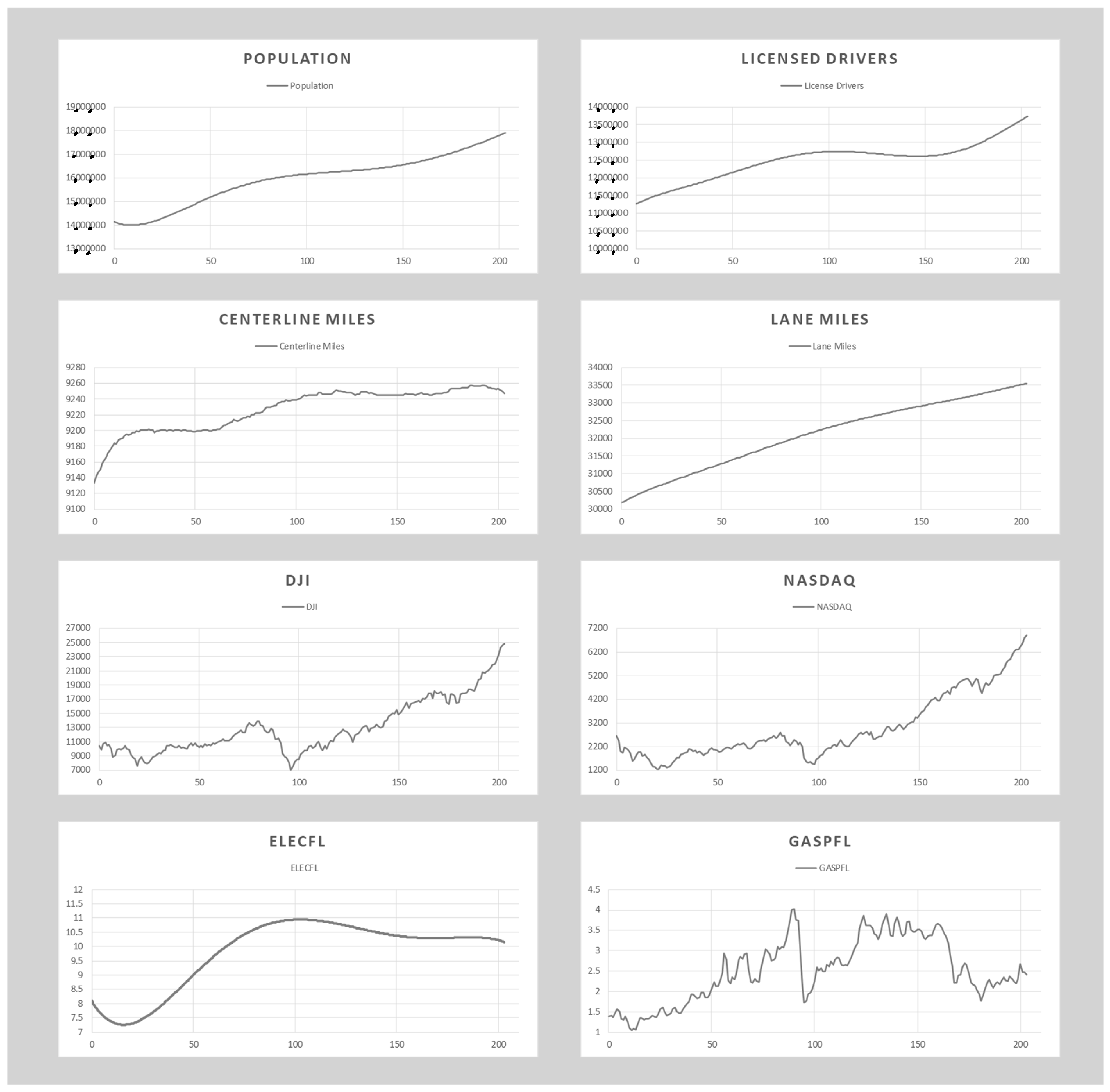


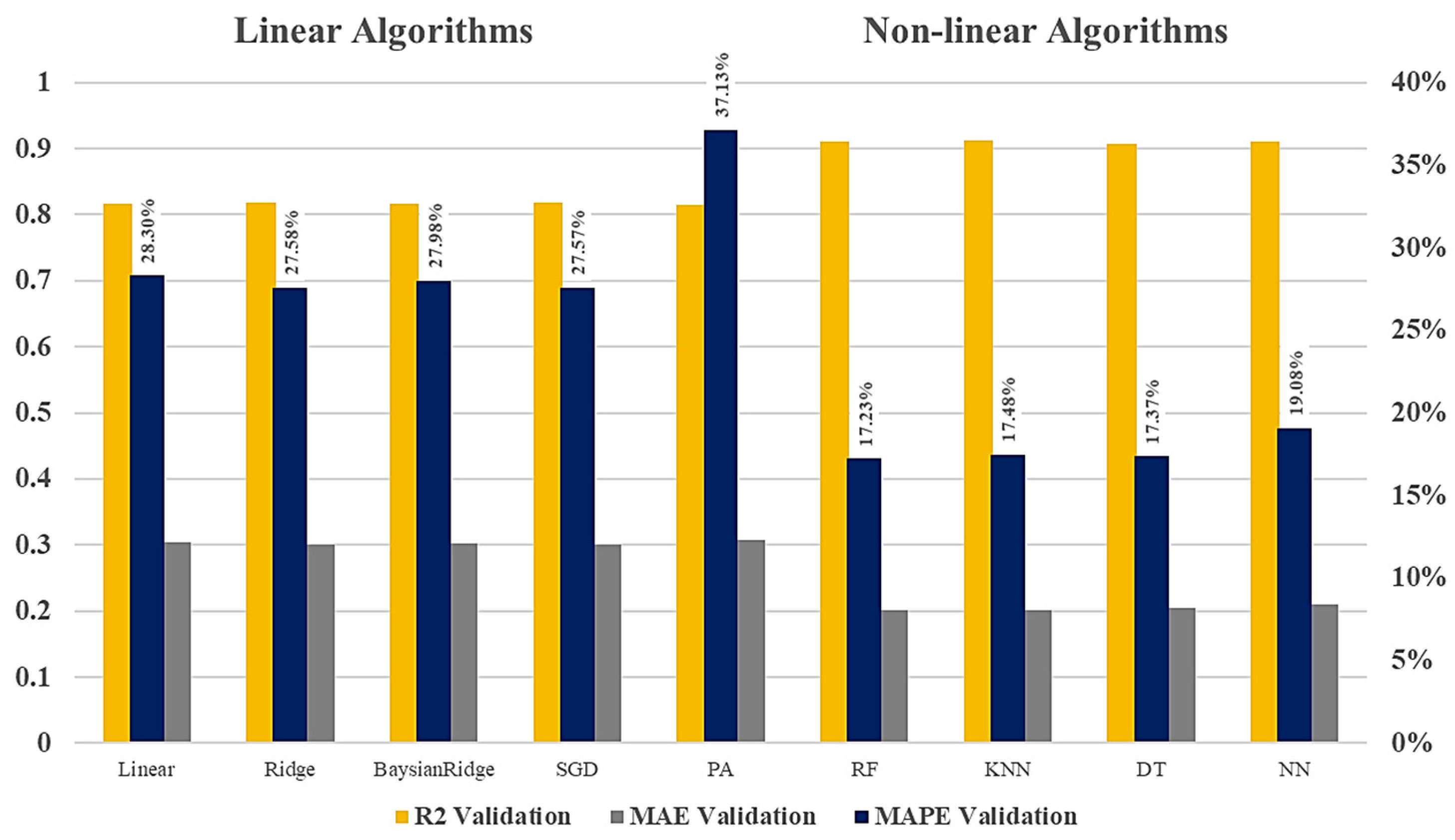

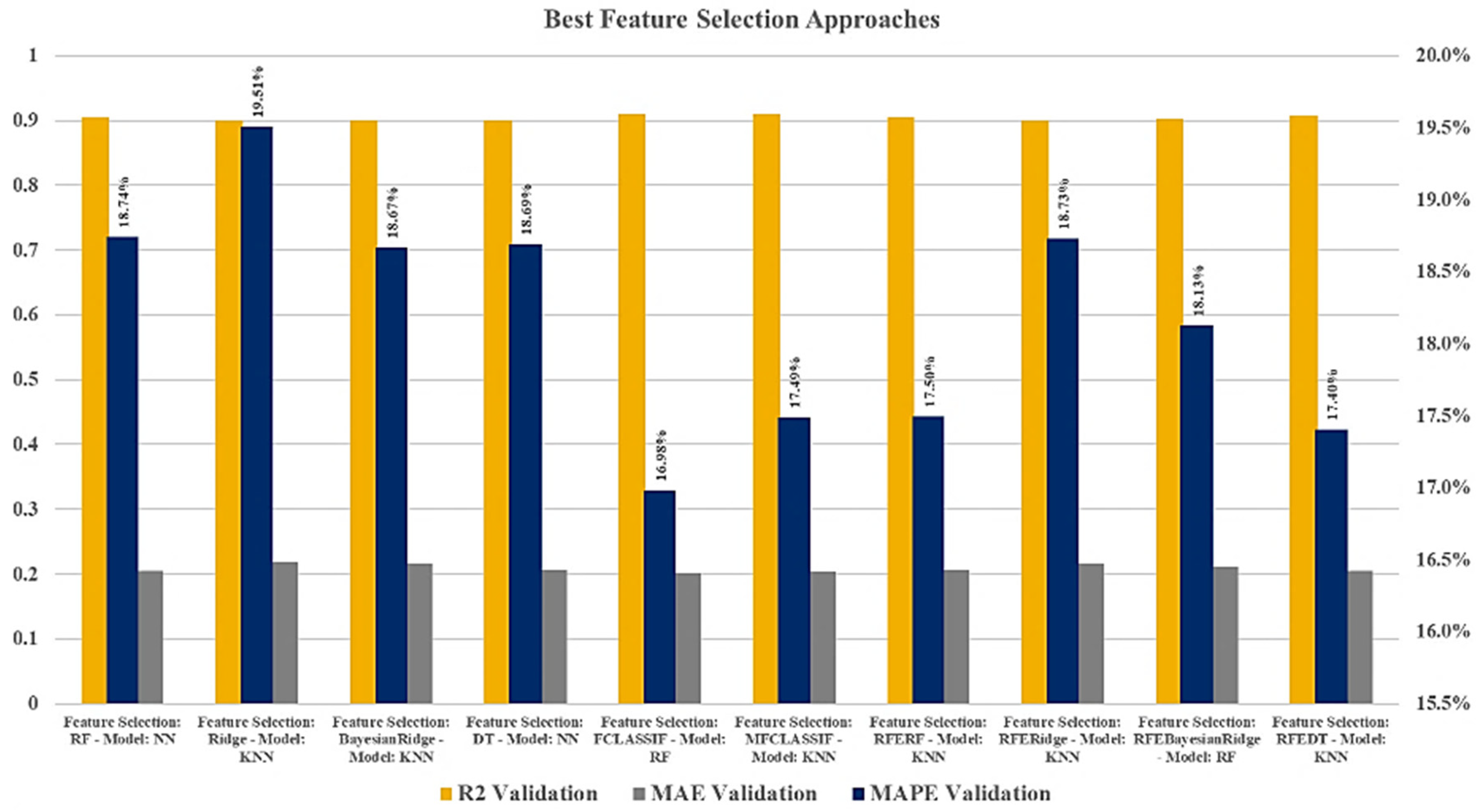
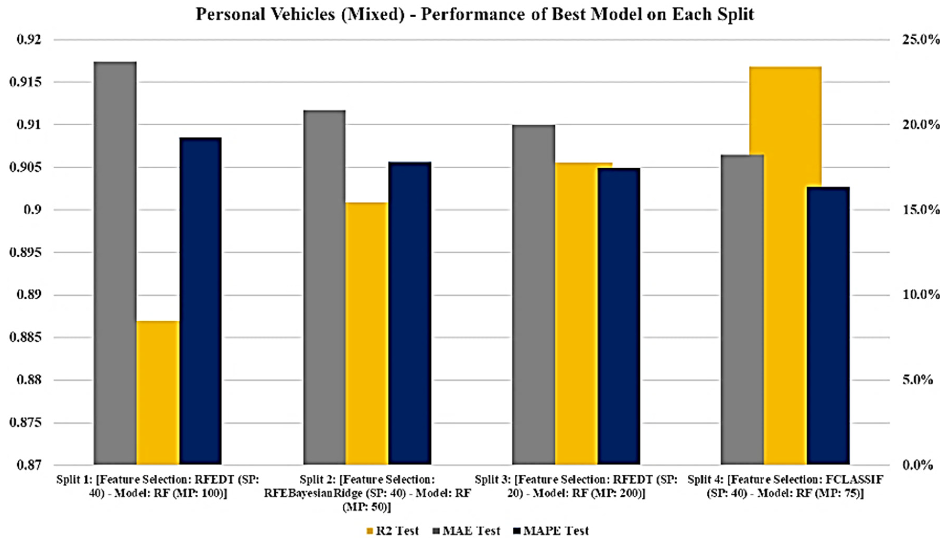


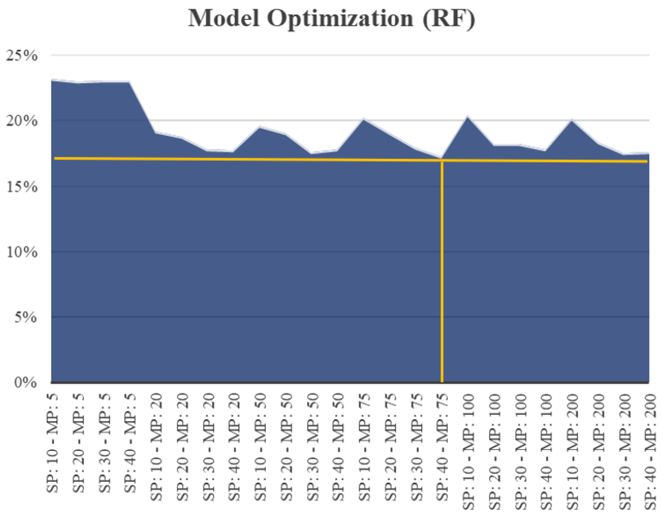
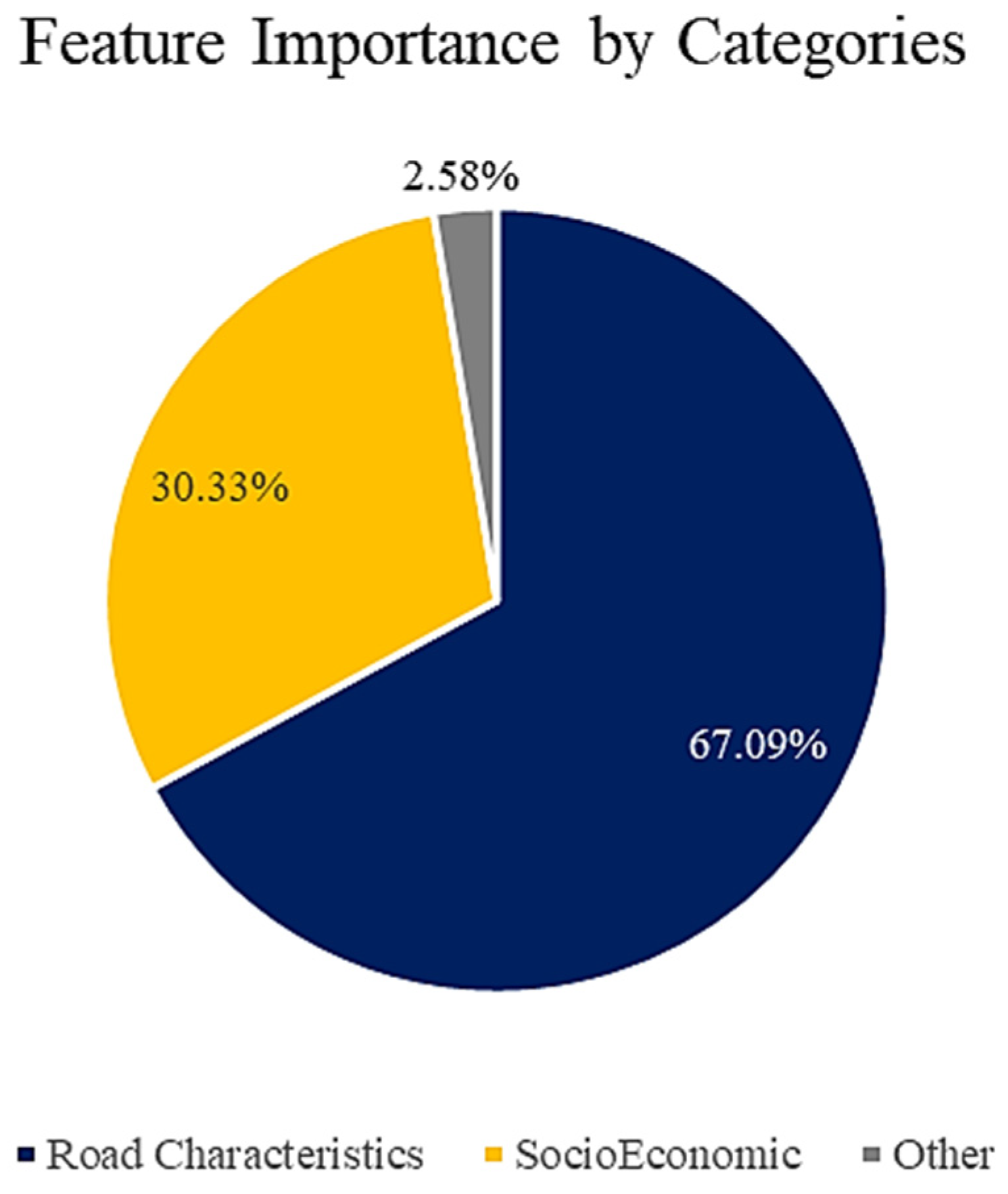

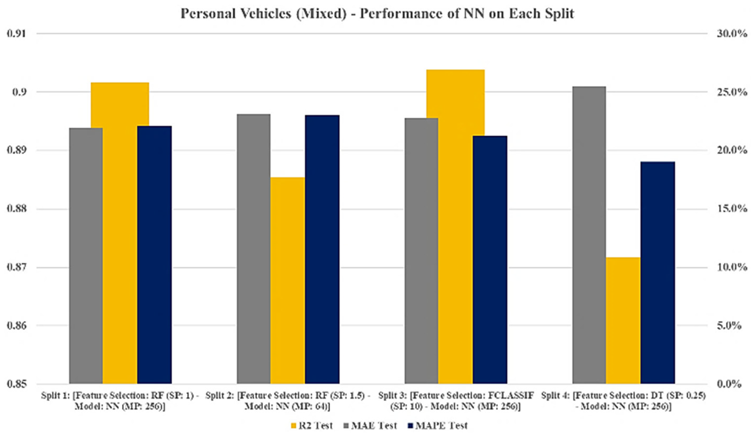


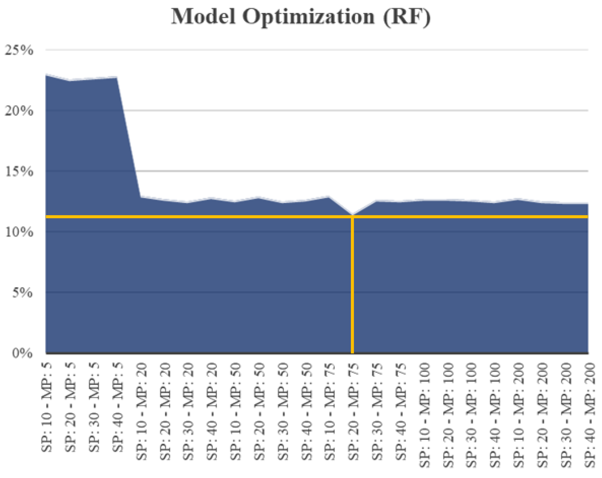


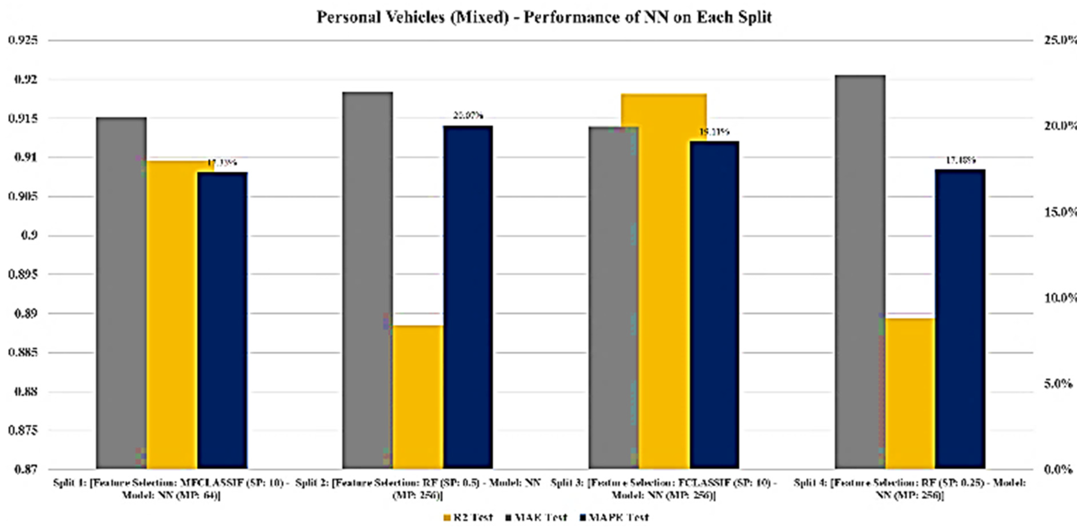


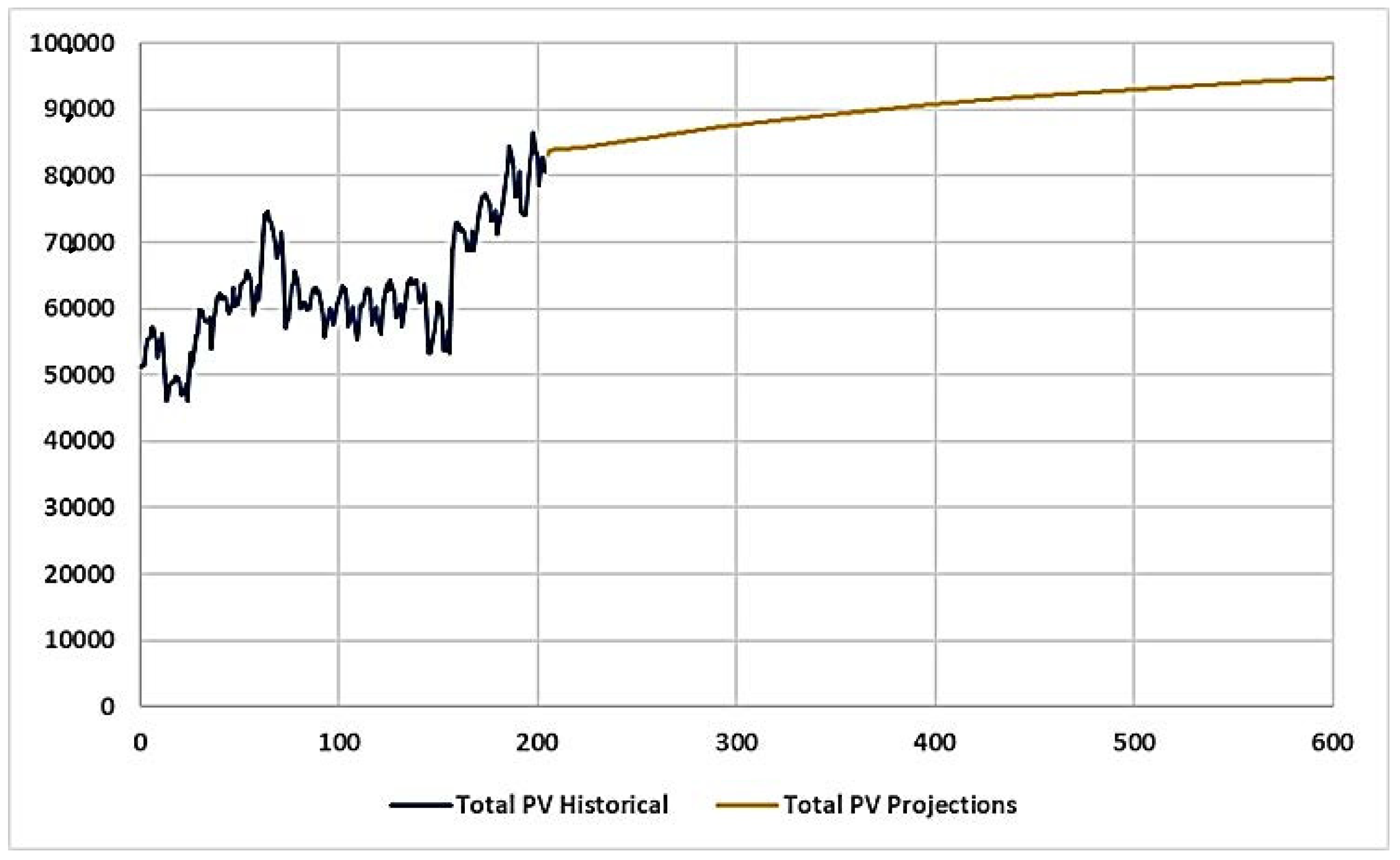

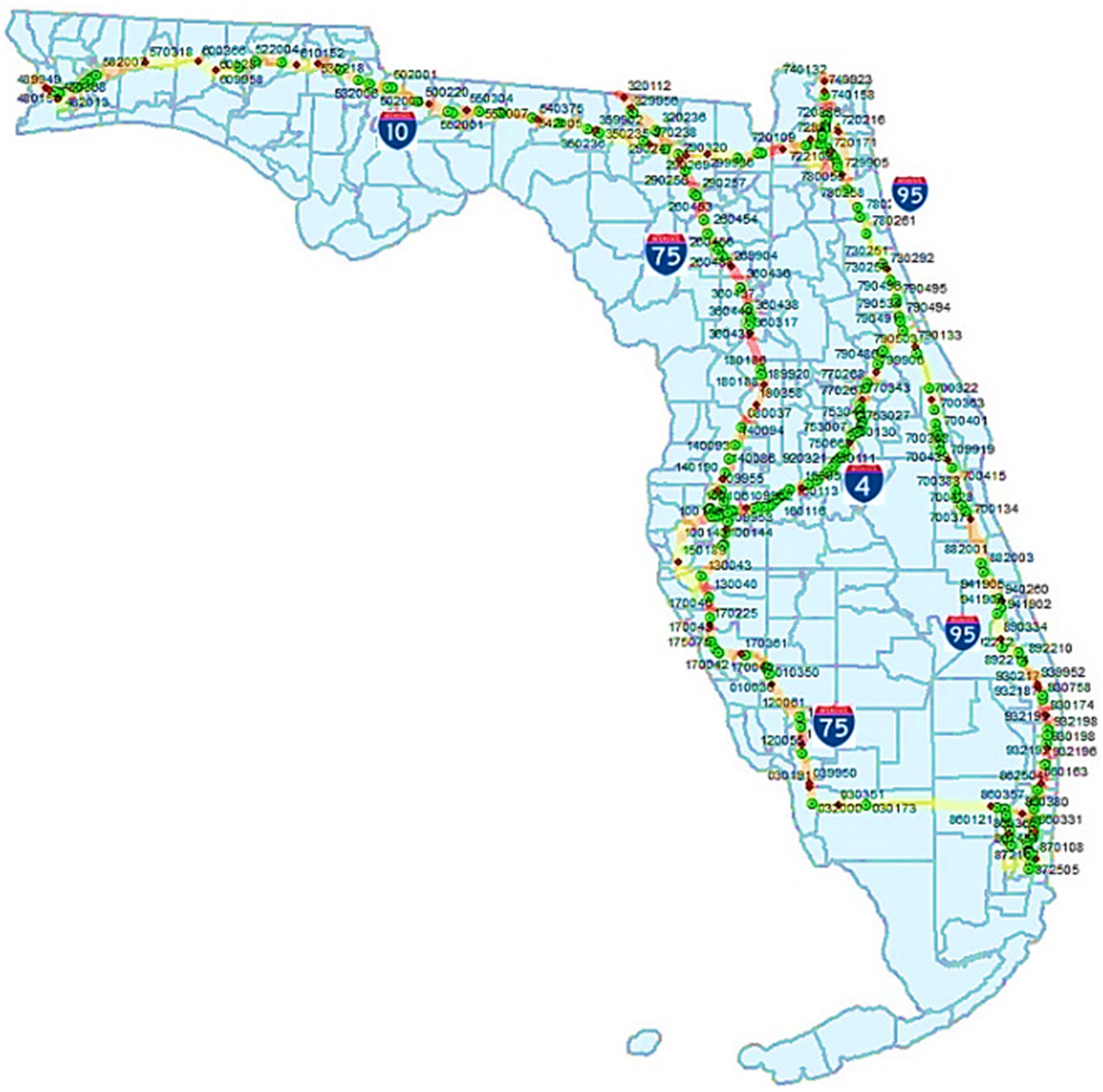
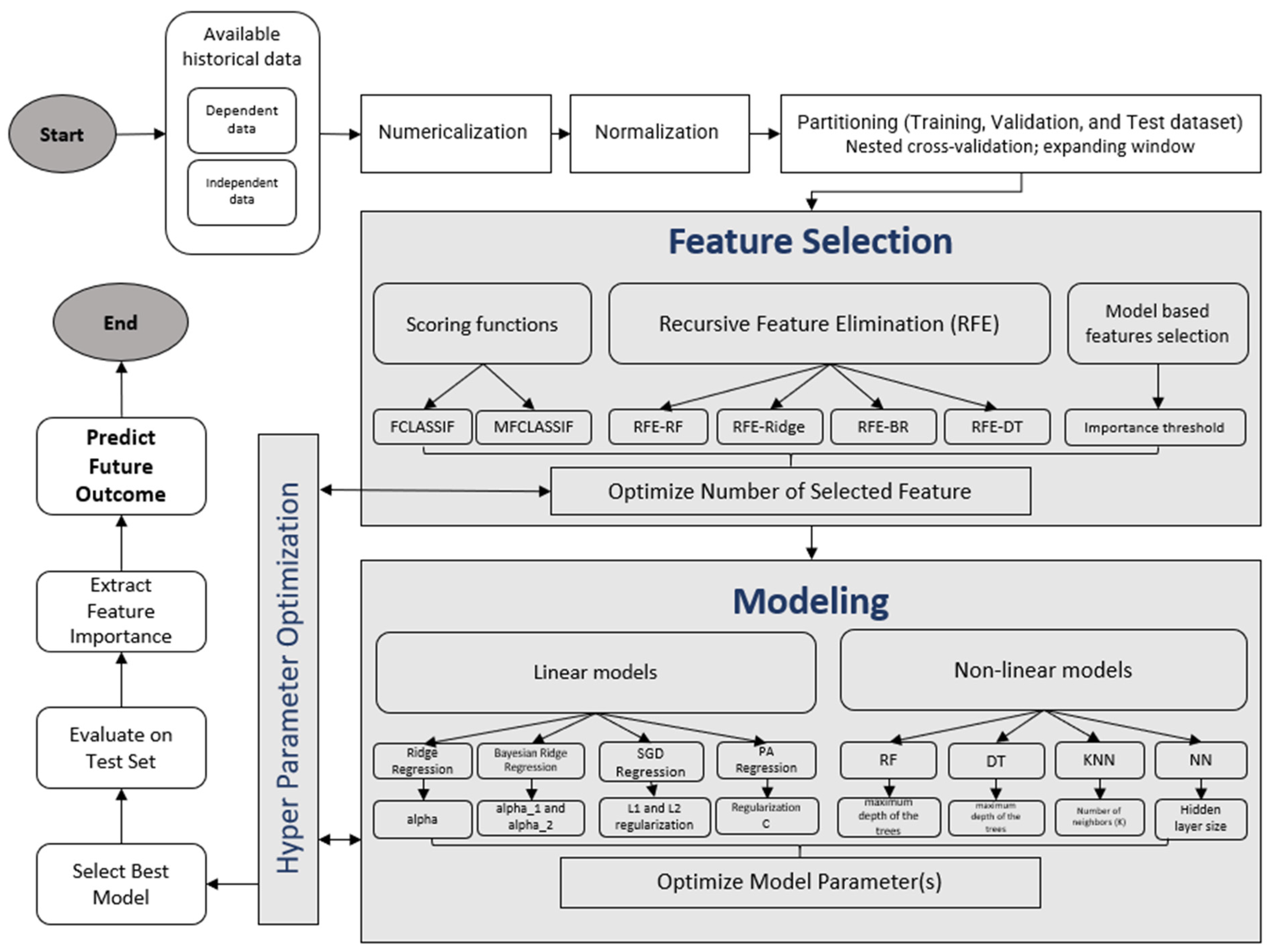
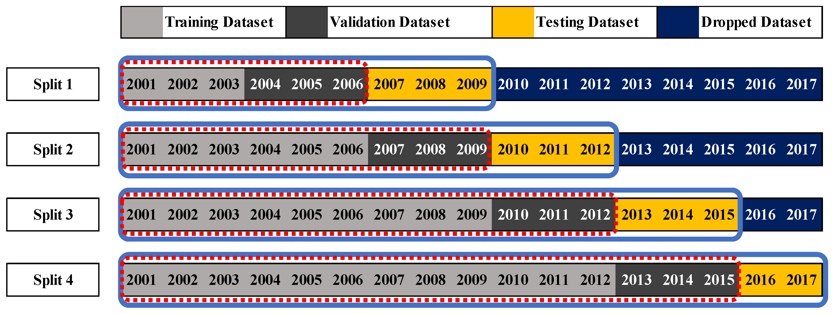
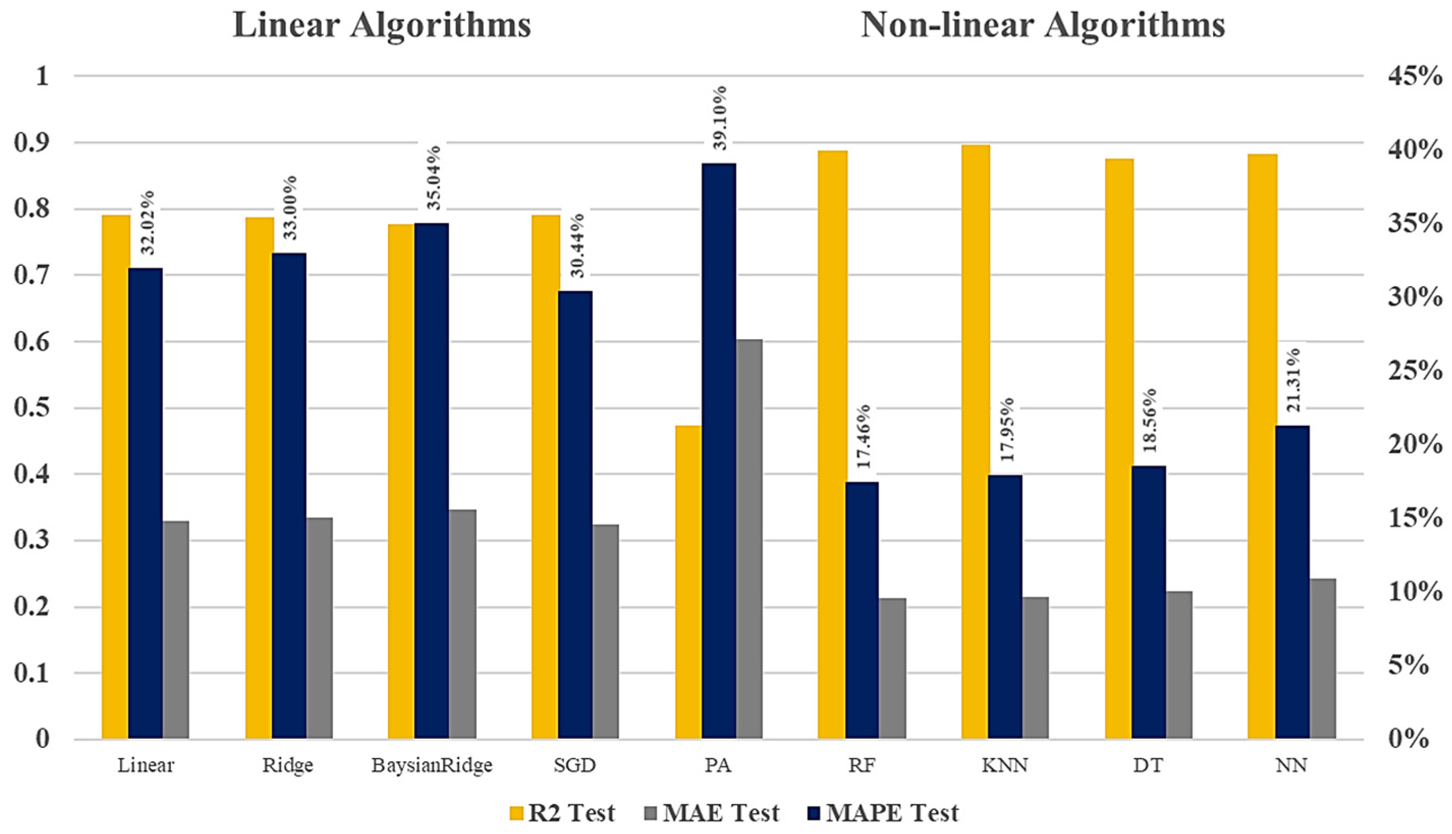
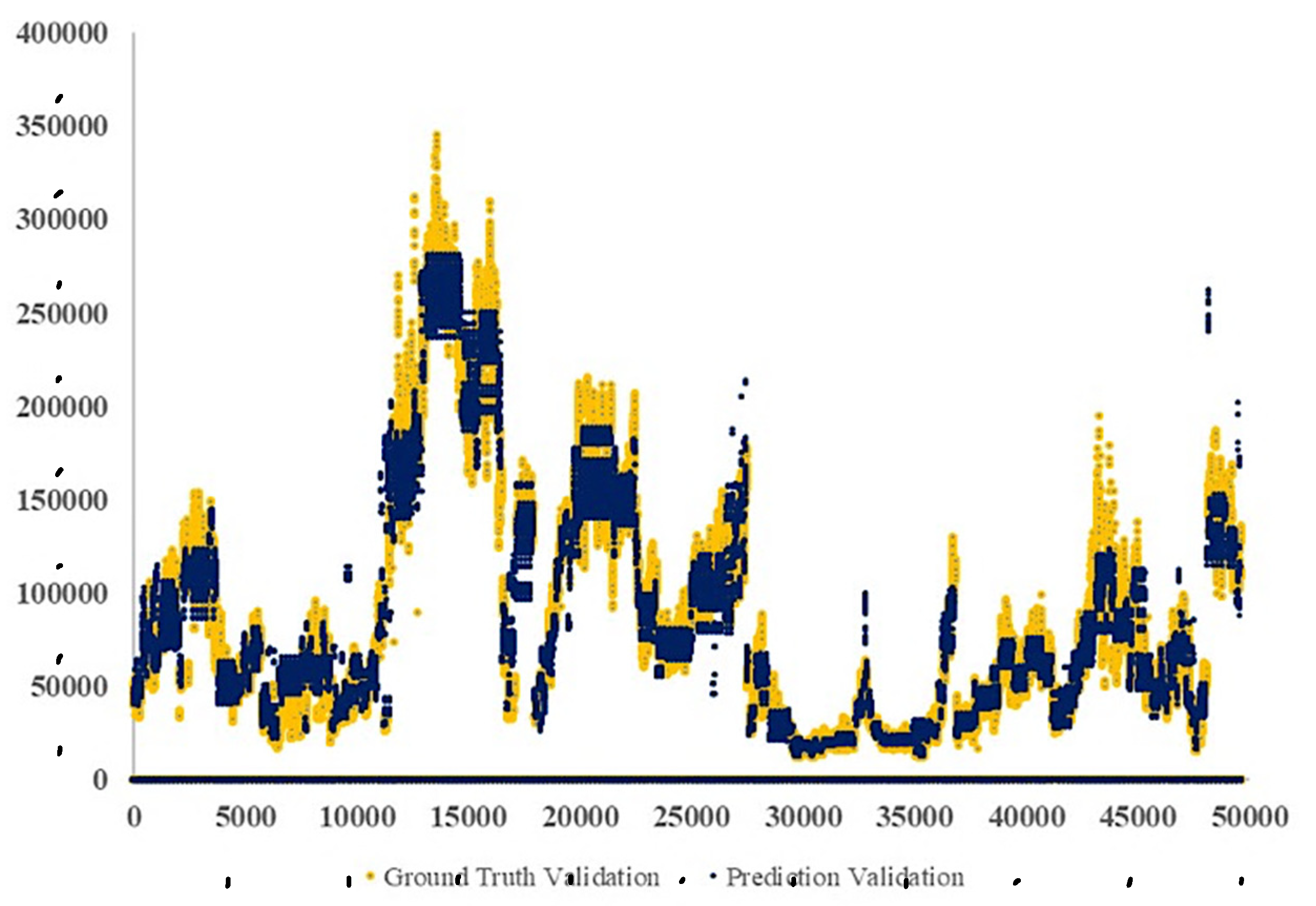
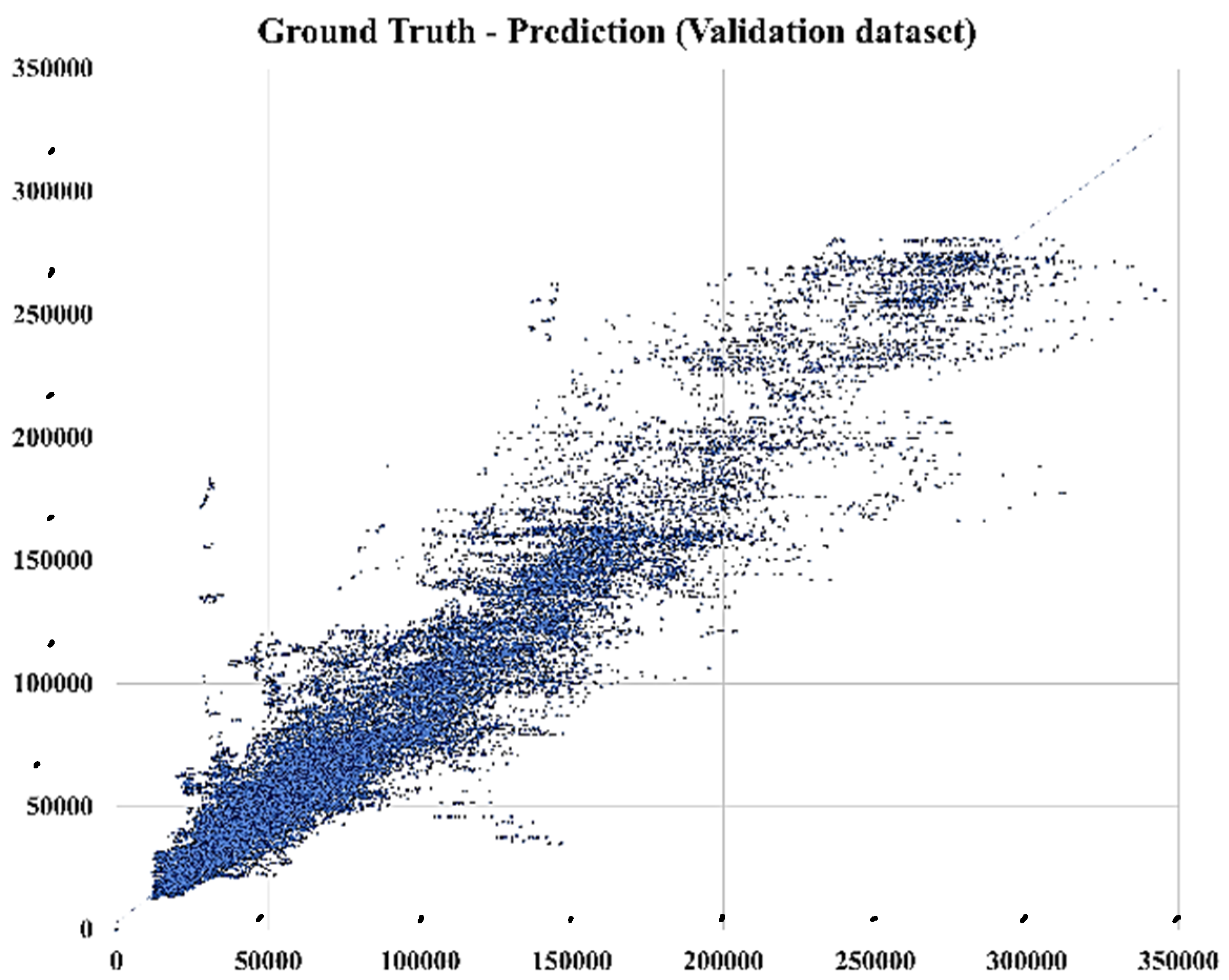
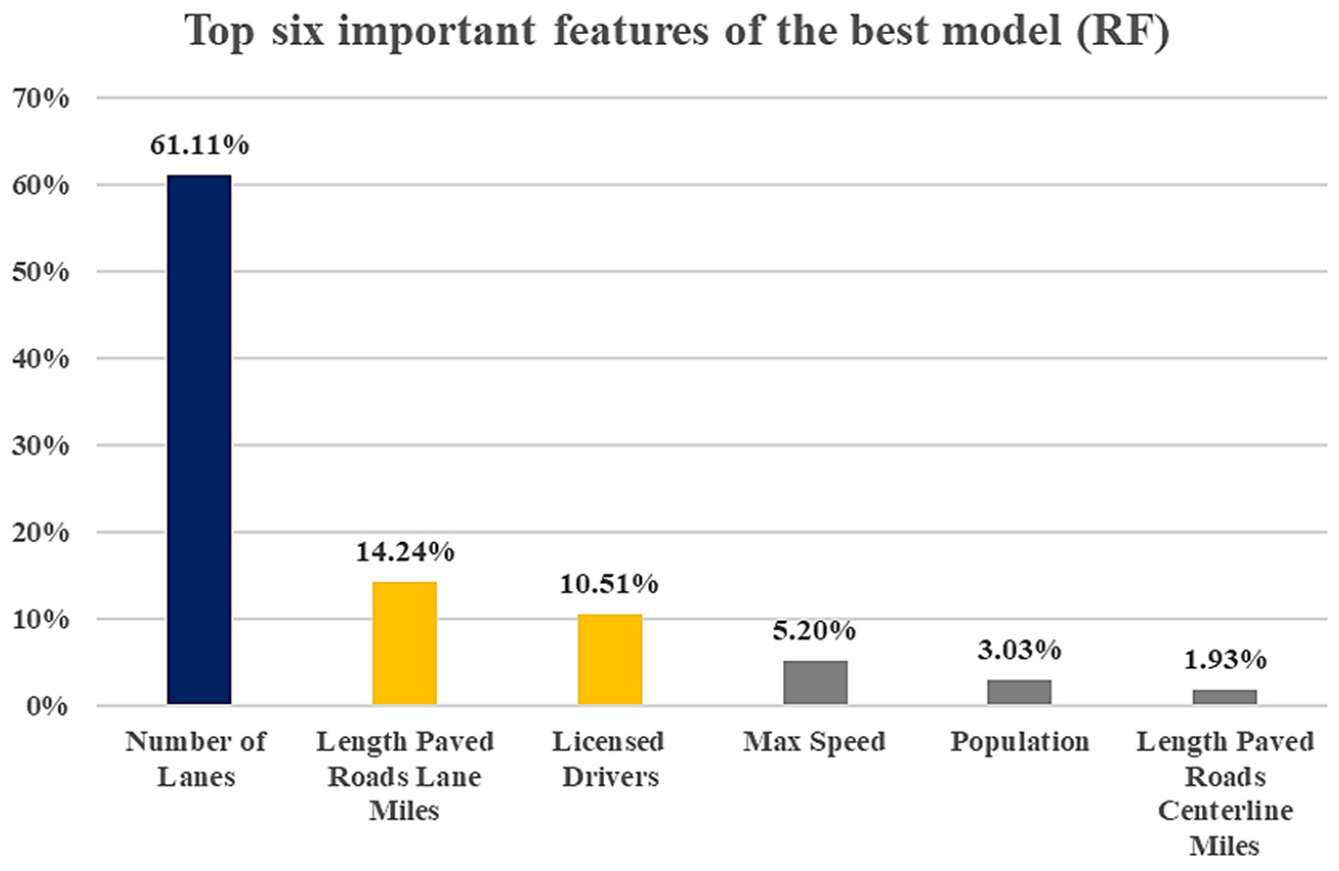
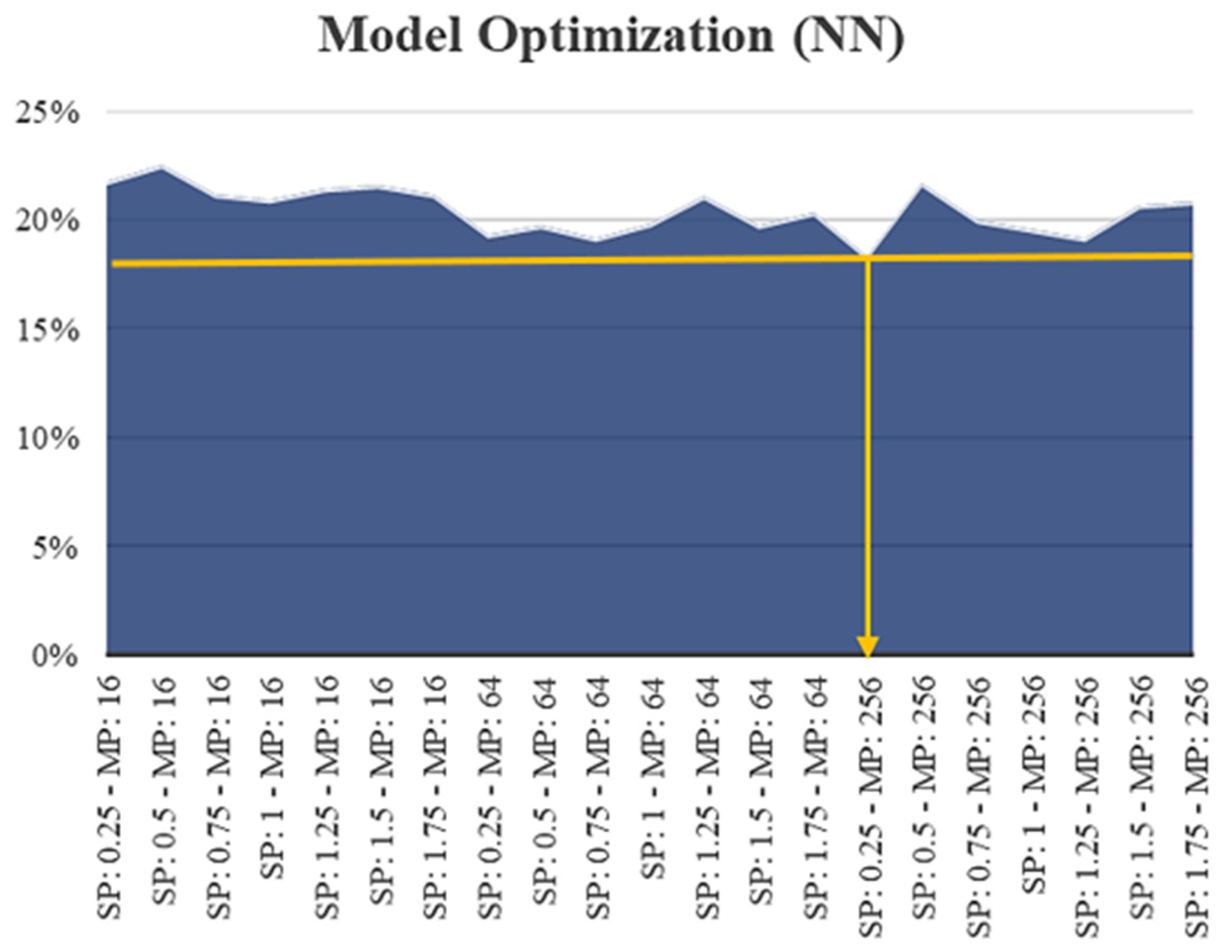
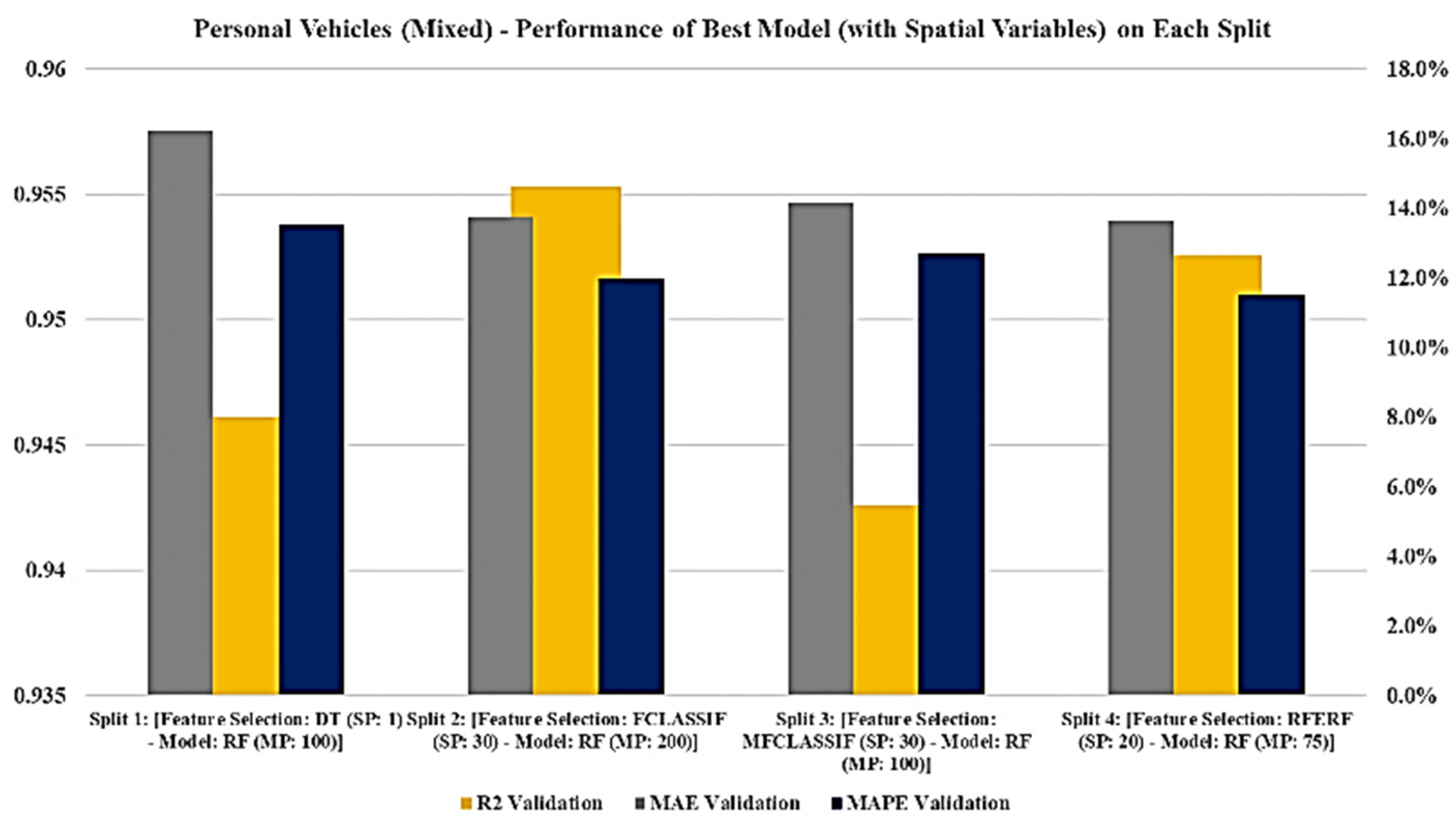
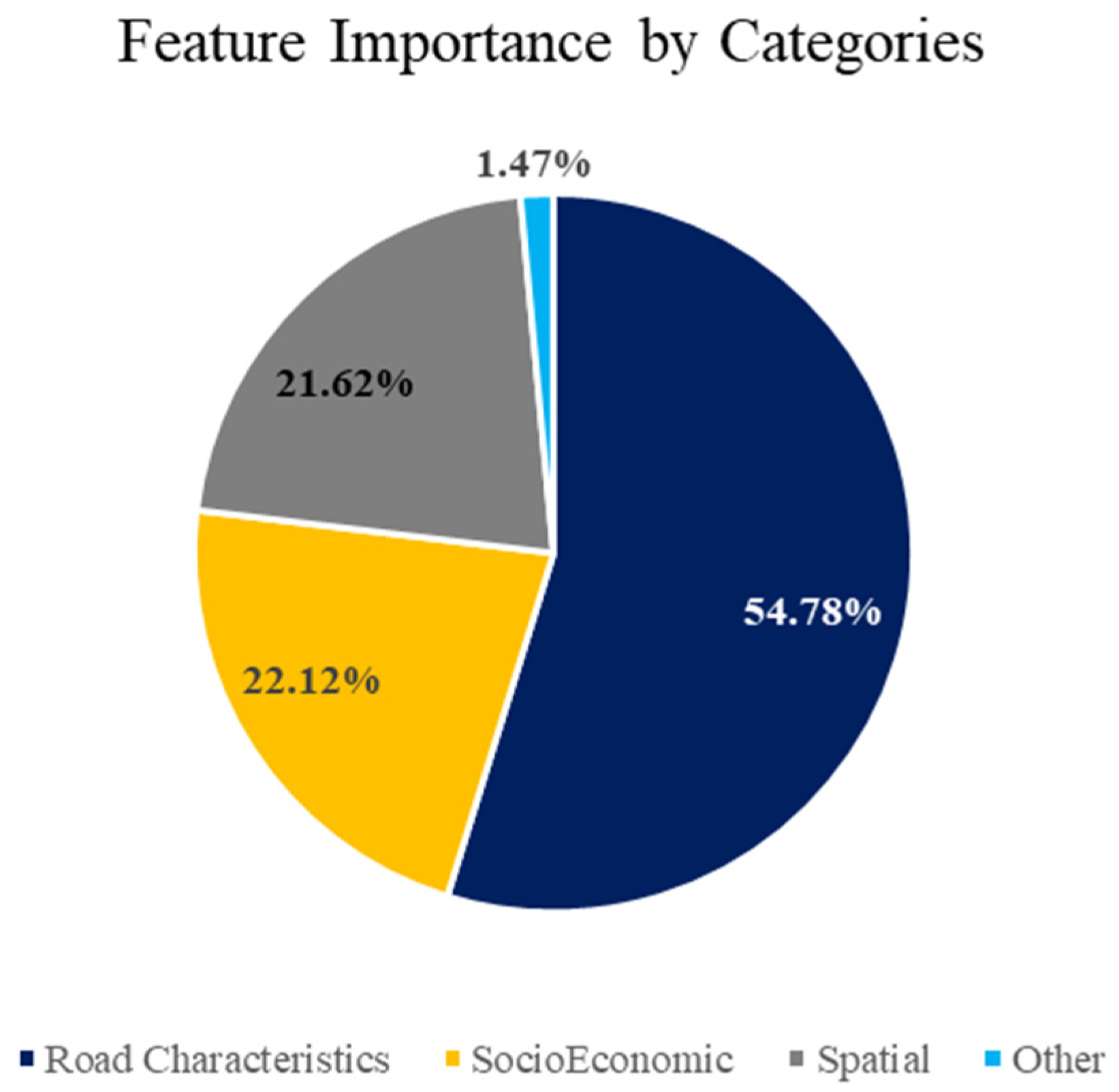
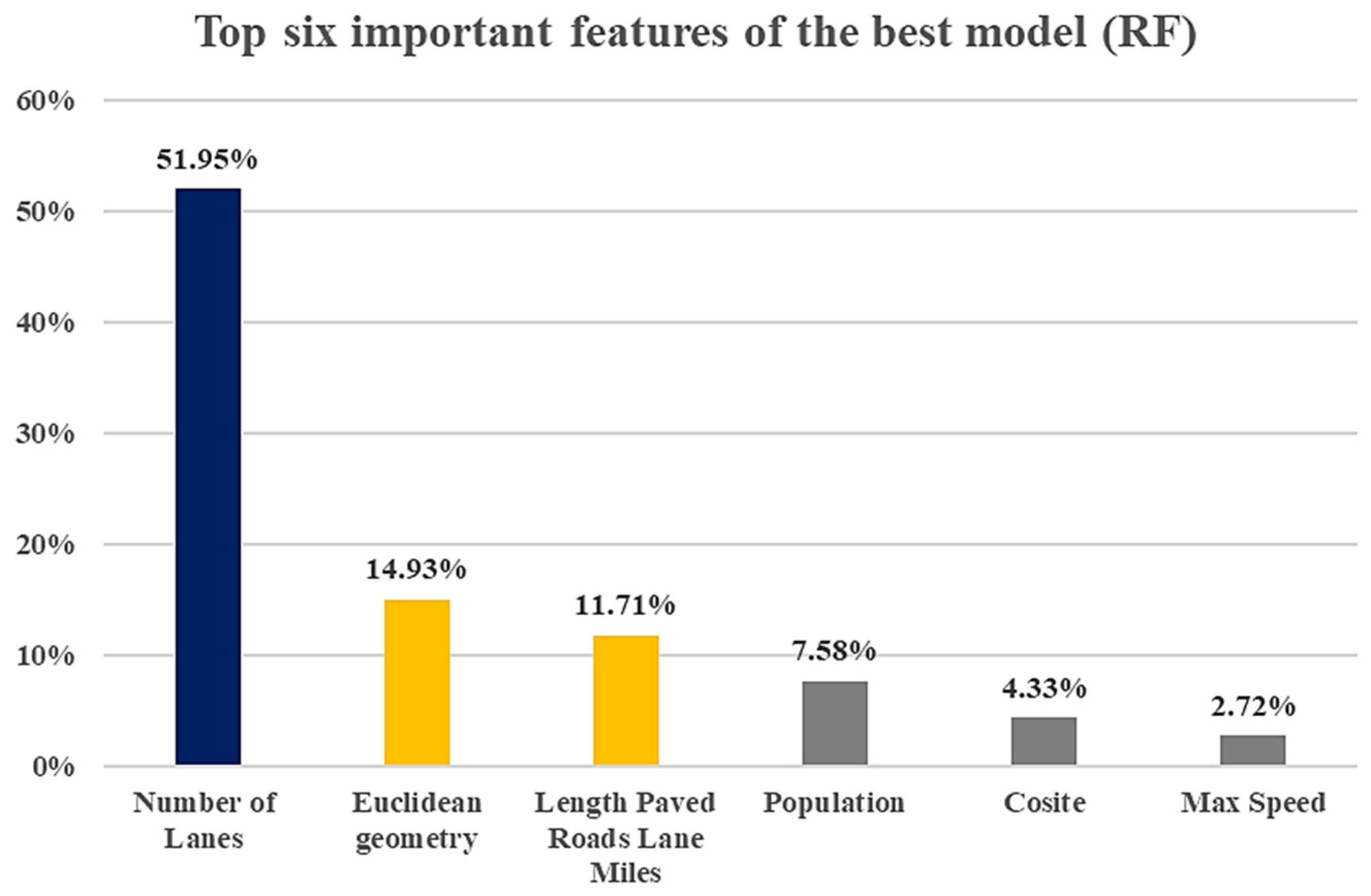
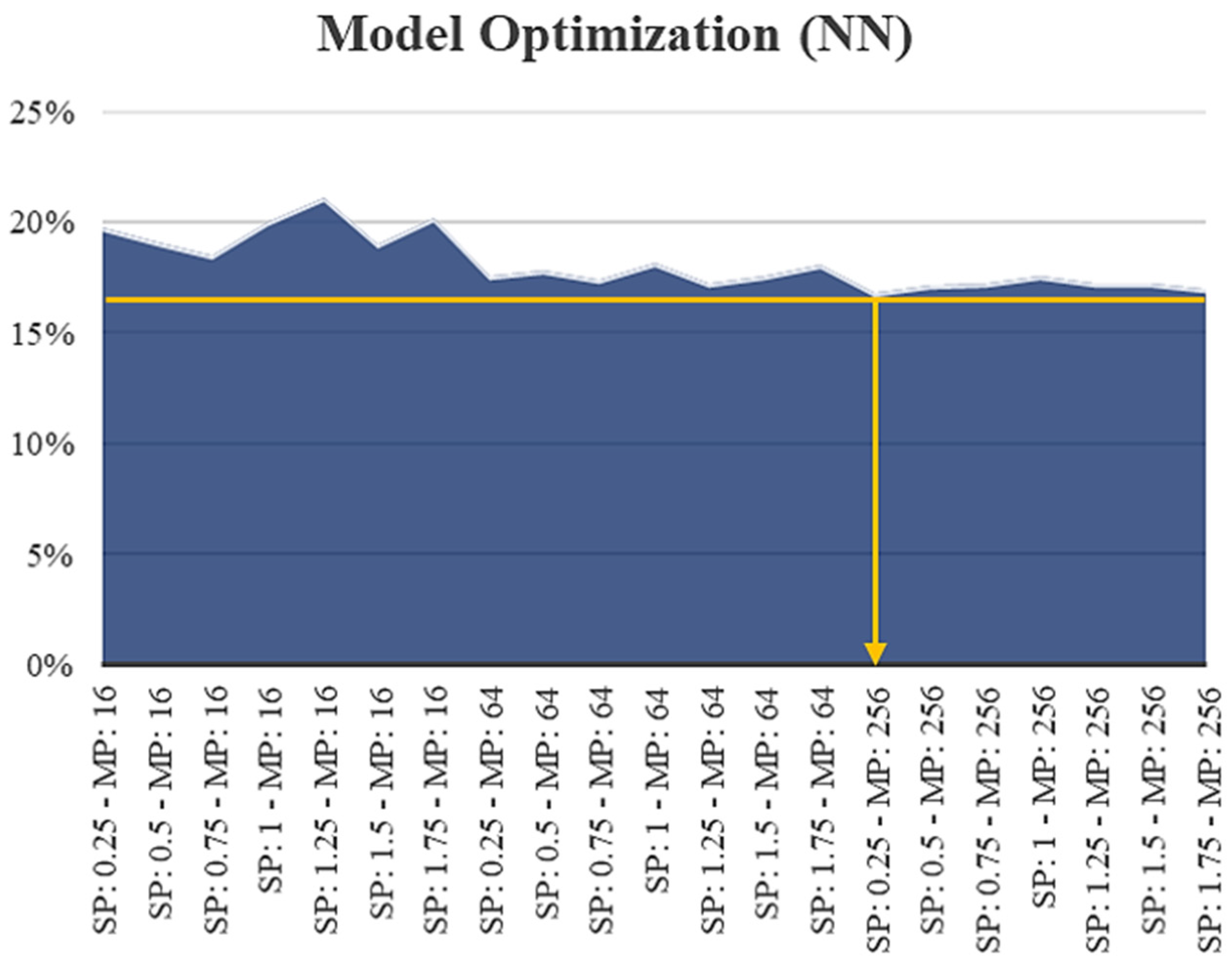
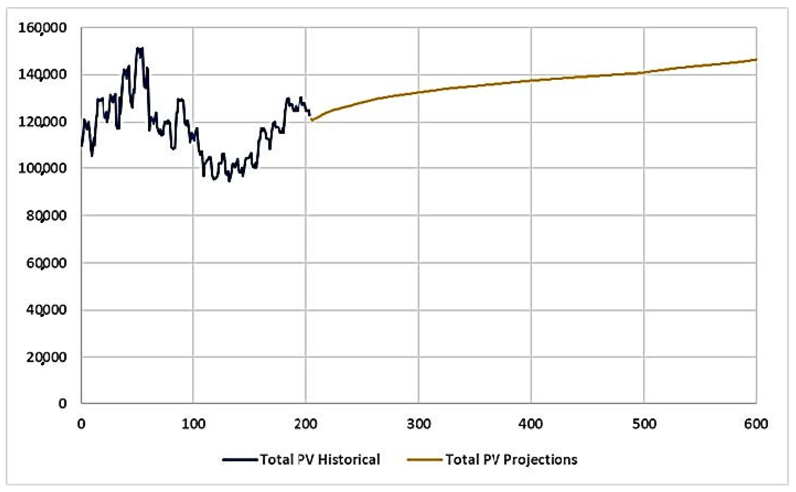
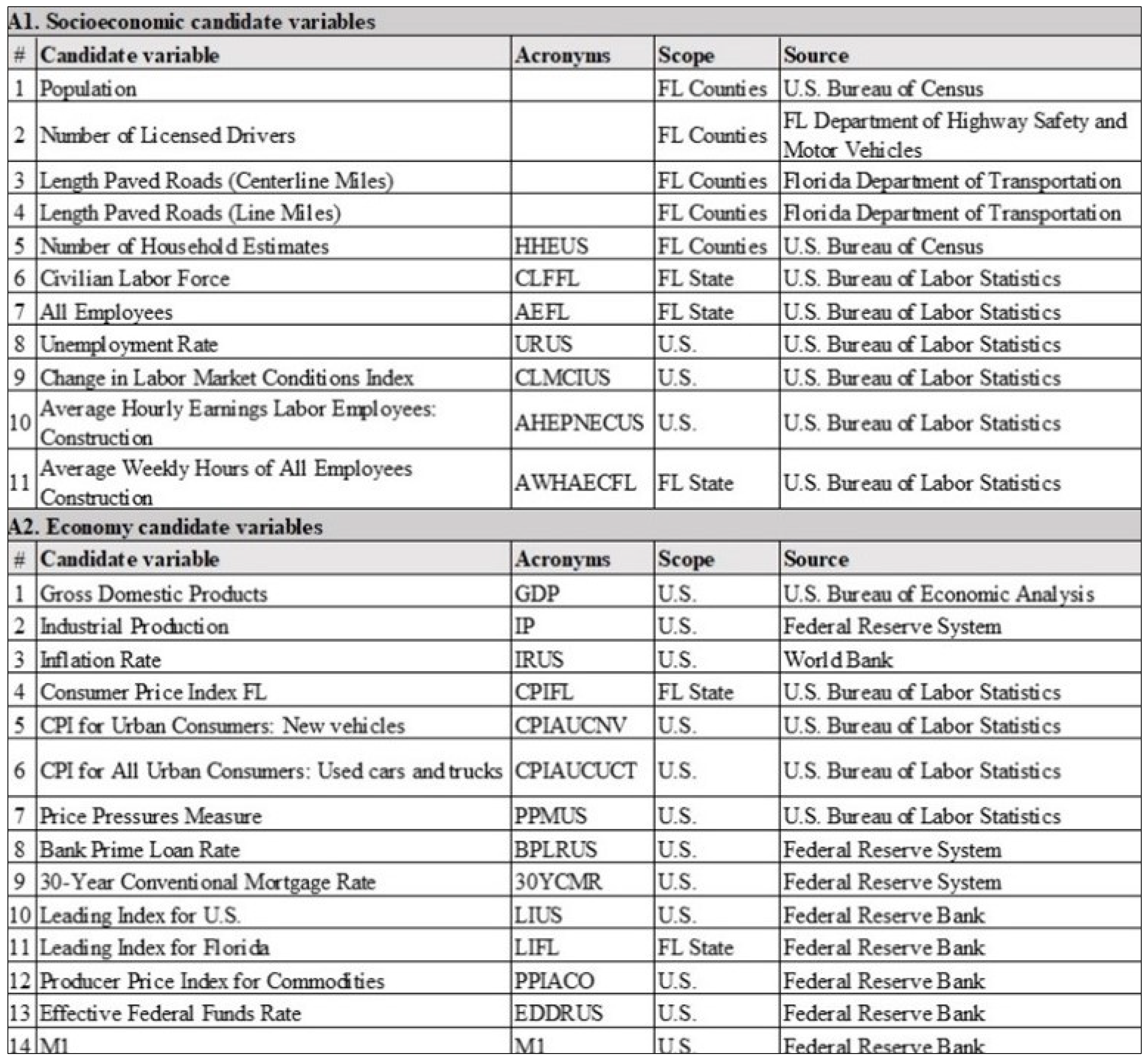
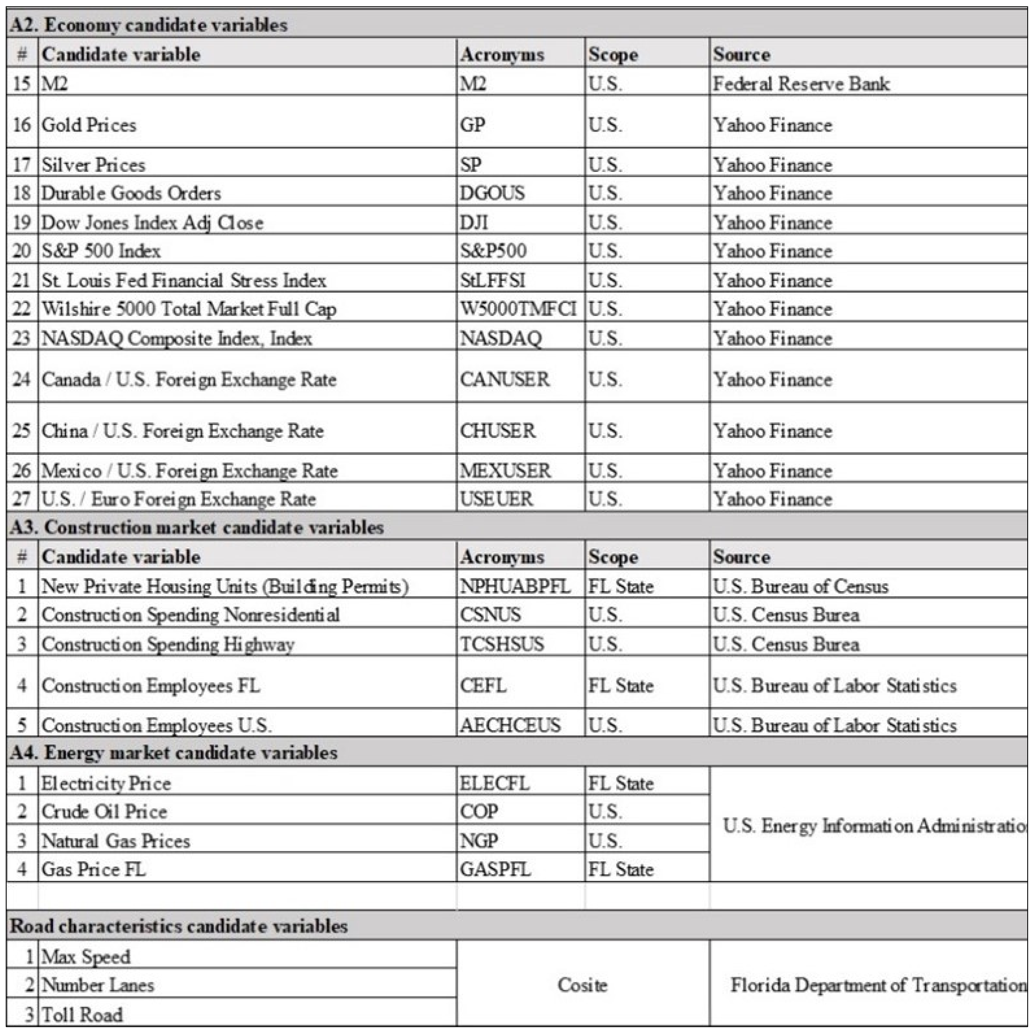