Explosives Use in Decommissioning—Guide for Assessment of Risk (EDGAR): I Determination of Sound Pressure Levels for Open Water Blasts and Severance of Conductors and Piles from Below the Seabed

Abstract

A simple underwater noise model suitable for use with explosives in the decommissioning of oil and gas subsea structures is introduced and evaluated against data from five projects in the US. The performance of the model is compared to four existing models for open water blasts, and for the severance of well conductors and piles. Simulated received underwater sound pressure levels were significantly correlated with measurements for all scenarios. The maximum total error achieved between simulations and measurements was 3.5%, suggesting that predictions are accurate to within 4% of the average measurement. A low relative bias was observed in the simulations when compared to measured values, suggesting only a small systematic underestimate (≤1% of average measurement) for most severance operations and a small overestimate (1.34%) for open water blasts.

1. Introduction

In the UK, the Department for Business, Energy and Industrial Strategy (BEIS) is responsible for permitting a varied array of offshore operations and ensuring that they are conducted in a safe, effective and environmentally sound manner. Several of these activities rely upon the underwater detonation of specialised explosive charges to perform specific functions [1]. These functions include the following:

• Perforation of well casings;
• Sound sources for geophysical surveys;
• Remote-/quick-release options (including via explosive bolts and pins, cable shearing devices, etc.);
• Down-hole drill pipe and casing cutting; and
• Severance of components such as piles, conductors and well stubs from subsea infrastructure during the decommissioning of offshore structures and wells.

Though several nonexplosive-severance methodologies can achieve the same goal (such as sand cutters, diver severance, abrasive water jet cutters, etc.), many operators feel that explosive-severance charges offer the most flexible, cost-effective, efficient and safest cutting options. However, despite their apparent advantages, the detonation of the explosives and the acoustic energy/shockwave released has the potential to injure or kill marine protected species, primarily marine mammals.

1.1. Explosion Dynamics

The features associated with the underwater detonation of an explosive charge include the explosion or detonation phase, the formation of the shock wave and its effects, the secondary loading effect known as bulk cavitation, the effects of the expanding and contracting gas bubble, observed surface effects and shock wave reflection and refraction effects [2].

A chemical explosion starts with an extremely rapid reaction that generates a large volume of high pressure, superheated gas. The pressure difference across the gas–water interface causes a steep-fronted shock wave, which moves directly outward at speeds greater than the speed of sound in seawater (~1500 m s⁻¹). The shock wave consists of a nearly instantaneous increase in pressure, which rapidly decays at a nearly exponential rate [3]. As the peak pressures increase, so does the speed of the shock wave. The peak pressure in the shock wave increases as the weight of the explosive charge increases and decreases as the shock wave moves away from the source.

The shockwave propagates spherically away from the source. This incident compressive shockwave (positive pulse) will intersect the air–water interface and be reflected as a tensile wave (negative pulse) [2]. The direct shockwave pressure will have begun to decay exponentially and on the arrival of the tensile wave, will abruptly further reduce the pressure to some negative value. In addition to these two loading effects, the shock wave also travels to the seabed. Depending on the nature of the bottom material, the resulting reflected wave can vary from a strong compressive reflection to a weak tensile reflection [2]. Multiple reflections (positive and negative), the result of successive reflections from the surface, seabed and other boundaries also occur.

When a compressive shock wave travels to the sea surface and is reflected as a tensile wave, a cavitation layer is formed at the air–water surface. An additional positive pulse, the bulk cavitation closure pulse is propagated once the cavitation bubbles collapse [2].

The hot gases from the chemical explosion also create a large, oscillating gas bubble in the water. The shock wave and the gas bubble each contain approximately half of the energy produced by the explosion. After the gas bubble is formed, it expands until the pressure inside the bubble is lower than the surrounding pressure. At that point, the bubble begins to collapse, causing the pressure inside to increase. This increase in pressure eventually causes the bubble to stop collapsing and to expand again. Pressure pulses are generated when the bubble begins to expand from its minimum volume. This bubble oscillation continues and creates a series of pressure pulses called bubble pulses. Each successive pulse is weaker than the preceding one. The peak pressure of the second bubble pulse is only about one-fifth that of the first bubble pulse. The shock wave propagation phase is in the order of milliseconds, while the bubble expansion and contraction phase are in the order of seconds [2].

If a fluid medium has varying thermal conditions, the assumptions of linear acoustic propagation of the incident shock wave begin to break down. The thermal gradients can bring about changes in the propagation speed and, thus, have the effect of causing the shock wave to bend along its path from the charge source to the target [2]. As a result, the propagation of the incident shock wave will be modified in terms of both speed and direction. Refracted shock wave paths may converge, focusing shock wave effects [2].

The scattering or absorptive effects of rough surfaces such as the sea surface or seabed can reduce the reflection coefficient for high frequency sounds [4].

1.2. Explosive Cutting

Explosions create a pressure impulse with a sharp rise time that is relatively broadband in frequency, including low-frequency energy. The spectral and amplitude characteristics of explosions vary with the weight of the charge and the depth of the detonation. The typical frequency range is 6 to 100 kHz, with near peak energy at frequencies of 10 to 200 Hz.

Nedwell and Edwards [5] found that peak pressure levels recorded during wellhead decommissioning were similar to those for similar explosive charges fired unconfined in the water. The charge was inserted into a casing and lowered to between two and three metres below the mud line. Nedwell and Edwards [5] suggested that the pipework surrounding the charge and the sediment below that the charge detonated did not act as an effective confinement for the blast. This may be understood from a physical point of view. First, the pipework surrounding the charge is in close proximity to the explosives and hence the forces acting on it are extremely high when compared with the burst pressure for the pipe. Second, the sediment adjacent to the pipe may be expected to be of comparable density to the adjacent water and hence the explosive energy will couple into the water as well in a similar way as it would when fired unconfined.

In one Gulf of Mexico (GOM) project, TAP-118 [6], the following two types of tubular members were explosively severed below the mud line: jacket leg piles and skirt piles, each consisting of a single layer of steel; and well conductors, each consisting of several concentric steel layers with grouting between layers. In addition, some of these structures had upper ends open to the air, whilst others terminated underwater. At 120 m from the platform, the shock parameters were less than 10% of the values expected at the same range from a free water Pentolite detonation of the same charge weight.

Pressures were reduced to 36% of the values observed at the same reduced ranges in free water in TAP-025 [7]. This was thought to represent a measure of the attenuation provided by mud and pipe confinement [6].

1.3. Problem Definition

The removal of offshore structures, for example, platforms, may involve the use of explosives to sever the following structure-associated components: wellheads, conductors, piles, etc. [4], at varying depths below the seafloor (mudline). The safest and easiest cutting procedure is to place an explosive charge inside tubing several metres below the mudline and sever the casing explosively.

The steep rises, high peaks and rapid falls in pressure caused by explosive cutting generates impulsive underwater noise and the impact from this will likely dominate any continuous noise sources, such as from vessels. The European Marine Strategy Framework Directive (MSFD) (2008/56/EC) suggested measures to assess underwater sound [8]. This assessment resulted in noise descriptors for low and mid frequency impulsive underwater sounds within the frequency range of 10 Hz to 10 kHz.

Government regulators and their advisers often need to understand the effects of anthropogenic underwater noise on marine species, especially marine mammals. However, many underwater noise simulation models, such as ARA [9], REFM (Britt et al., 1991, as cited in [9]) and CASS/GRAB [10], are exceedingly complex, requiring too many parameters to be used by non-specialists.

Currently, many underwater noise models are propriety and/or black box. Indeed, the practice of underwater noise modelling is inconsistent amongst and between environmental consultants, oil and gas operators and regulators. It is timely for an open-source model to be developed and evaluated. This model should be as simple and transparent as possible to enable easy use by stakeholders.

If a relatively simple, transparent, fit-for-purpose model can be realised, this could help industry access the science, reducing consultancy, regulator and operator decommissioning costs.

1.4. Innovation

Here, a simple underwater noise model, “Explosives use in Decommissioning—Guide for Assessment of Risk (EDGAR)”, is introduced, which can be implemented using only the limited information available for the modelling required by regulators. EDGAR has been written in Microsoft Excel so that it is transparent and easily accessible for different uses by regulators, the industry and other researchers. The model combines a new formulation of existing underwater noise models with a novel method based on the dynamic pattern of curve fits from the existing more complex models.

For impulsive sound, it is important to consider the peak sound pressure levels (SPL_pk thresholds), which can induce TTS or PTS regardless of its energy and frequency content [11]. EDGAR Part I details the development of a simple transparent model for the determination of SPL by inputting the explosive charge weight. The SPL model has been evaluated against data from several decommissioning projects using explosive severance in the GOM.

The underwater noise model is evaluated against peak pressure data from explosive decommissioning projects in the Gulf of Mexico. Note that these were the only relevant data and associated models that were available at the time of writing.

1.5. Aims

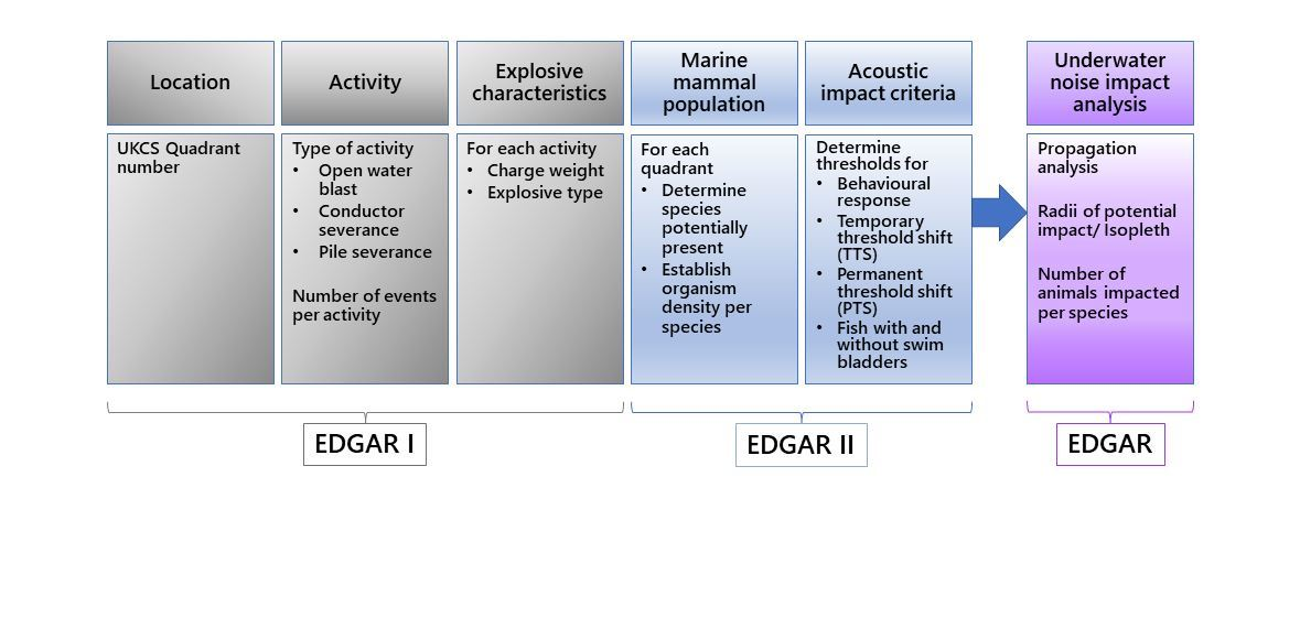
The aims of this study are to (1) describe the structure of the underwater noise model, (2) explain the methodology developed to initialise and run the model and (3) present an evaluation of the underwater noise model. This study is documented in the following two parts: EDGAR Part I relates to the generation and propagation of underwater sound (current study), and EDGAR Part II [12] focuses on exposure to underwater noise and the potential environmental impact on receptors.

2. Materials and Methods

2.1. Sound Propagation

As sound spreads underwater, it decreases in strength with distance from the source. This transmission loss is the sum of spreading loss and attenuation loss. Attenuation losses are the physical processes and conditions in the sea that weaken the sound signal. These factors include sound absorption or scattering by organisms in the water column, reflection or scattering at the seabed and sea surface and the effects of temperature, pressure, stratification and salinity. Variations in temperature and salinity with depth cause sound waves to be refracted downwards or upwards causing increases or decreases in sound attenuation and absorption. This leads to actual sound transmission having considerable temporal and spatial variability that is difficult to quantify.

2.2. Model Development

In this section, several important measures of sound will be discussed. The maximum absolute pressure within a particular time interval is known as the peak level. The source level is the strength of an acoustic source. The higher the source level is, the louder the sound that the source produces is. However, the larger the distance from the source is, the lower the level that is experienced is. This location-specific measure for received sound, the sound pressure level is indicative for an average level of sound that is present at that location. The total cumulative amount of sound that is received in a given period of time is the sound exposure level.

2.2.1. Shockwave Pressure

In the very near-field, the shock pulse pressure given as a function of time $p\left(t\right)$, in Pa, consists of a near-instantaneous increase in pressure followed by an exponential decay, as follows [13]:

$$p\left(t\right)=p_{0}exp\left(-t/t_0\right)$$

(1)

where $p_0$ is the peak pressure (Pa) associated with the shock front and $t_0$ is a time constant for exponential decay (s). Explosion shock theory has proposed specific relationships for the peak pressure and time constant (Section 2.2.2) in terms of the charge weight and range from the detonation position.

In the vicinity of an underwater detonation, the “near-field”, the peak pressure, $p_0$, in Pa, can be estimated by the following power law [13,14]:

$$p_0\left(r\right)=K_p{\left(\frac{W^{1/3}}{r}\right)}^{{\alpha }_p},$$

(2)

where $W$ is the charge weight (kg), $r$ is the distance from the detonation (m) and $K_p$ and ${\alpha }_p$ are empirical parameters that depend on the explosive type. (In this study, the parameter values used were $K_p=5.24\times {10}^7$ and ${\alpha }_p=1.13$ for open water blasts.)

The power law relationship is generally found to be valid in the near field [15], up to a limit of

$$r_0=4.76W^{1/3}\mathrm{m}.$$

(3)

Beyond this limit, the theory of weak shock propagation [16] is appropriate. In this regime the peak pressure is given by the following:

$$p_0\left(r\right)=p_0\left(r_0\right)\left\{\left[{\left(1+2\frac{r_0}{L_0}ln\left(\frac{r}{r_0}\right)\right)}^{0.5}-1\right]/\left(\frac{r}{L_0}ln\left(\frac{r}{r_0}\right)\right)\right\}$$

(4)

where the characteristic distance, $L_0$, (m) is as follows:

$$L_0=\frac{\rho c_w{}^3{t}_0\left(r_0\right)}{p_0\left(r_0\right)\beta }$$

(5)

where the density of seawater, $\rho \approx$1027 kg·m⁻³; the speed of sound in seawater, $c_w\approx$1500 m·s⁻¹; a dimensionless acoustic nonlinearity parameter for water, $\beta$ = 3.5; and $p_0\left(r_0\right)$ (Pa) and $t_0\left(r_0\right)$ (s) are computed from the near-field equations (Equations (2), (3) and (6) (top)). The similitude equations for time [4,13,16] are as follows:

$$t_0\left(r\right)=\left\{\begin{array}{ll}{K}_t{W}^{1/3}{\left(\frac{W^{1/3}}{r}\right)}^{{\alpha }_t}& \mathrm{if}r\le r_0\\ t_0\left(r_0\right){\left(1+2\frac{r_0}{L_0}ln\left(\frac{r}{r_0}\right)\right)}^{0.5}& \mathrm{if}r>r_0\end{array}\right.$$

(6)

where $K_t$ and ${\alpha }_t$ are empirical parameters that depend on the explosive type. (In this study the parameter values used were $K_t=8.4\times {10}^{-5}$ and ${\alpha }_p=-0.23$.)

As the shockwave propagates, the peak pressure declines, and the exponential decay becomes more gradual.

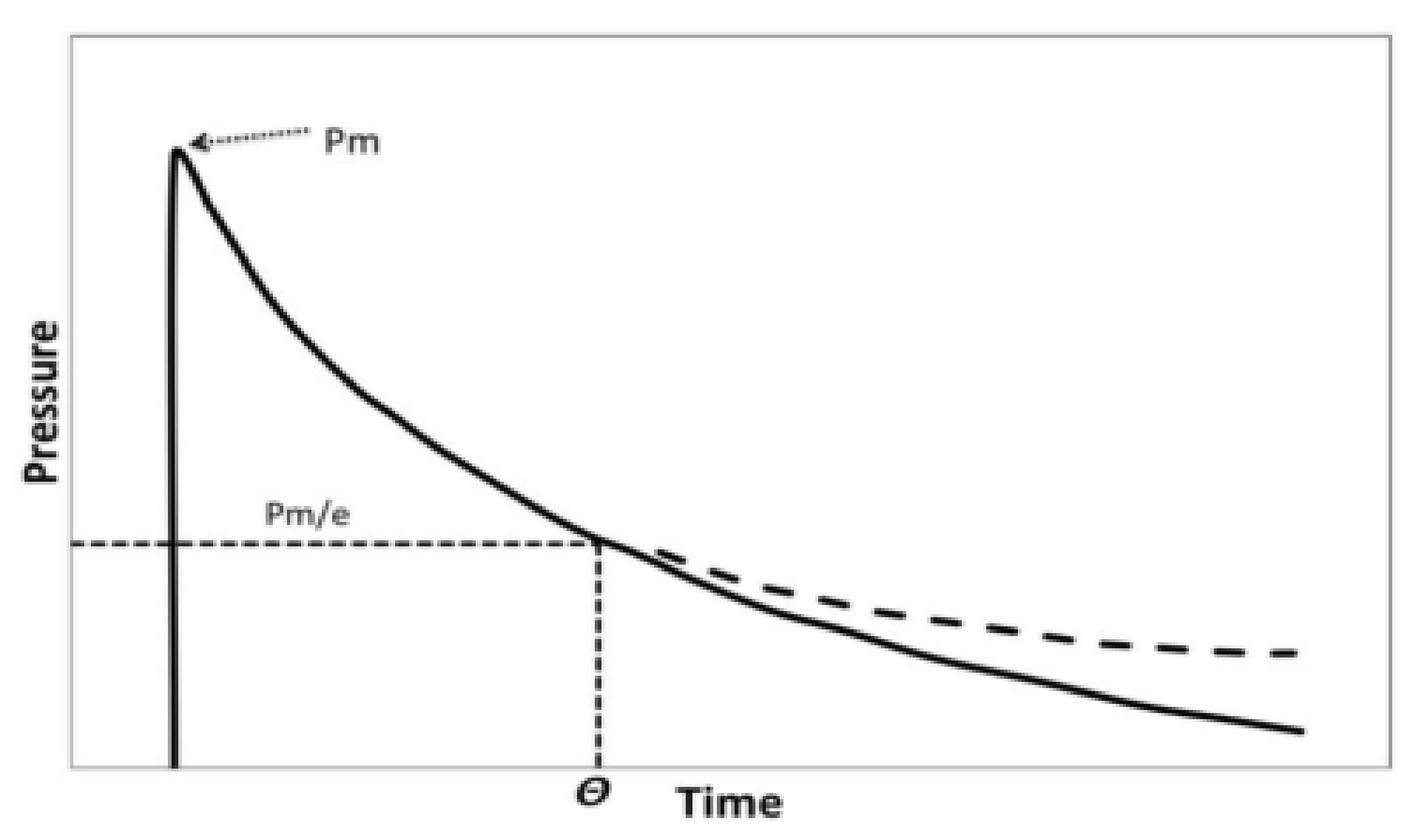
2.2.2. Time Constant

The time constant, $\theta$, is defined as the time needed for the peak pressure (P_m$=p_0\left(1\right)$) to decay to the defined value of P_m/e, where e ~2.718 [17]. Hence, the time constant, $\theta$, (s) can also be defined as given in Equation (6) (top) as follows:

$$\theta =K_t{W}^{1/3}{\left(\frac{W^{1/3}}{r}\right)}^{{\alpha }_t}$$

(7)

where $K_t$ and ${\alpha }_t$ are empirical parameters that depend on the explosive type.

Figure 1 illustrates the procedure to determine the time constant (redrawn from [3]). The solid line represents exponential decay. As per Swisdak [3], exponential decay is expected to occur until about one time constant ($\theta$). After that, the actual decay in pressure is expected to occur more slowly, shown as the dashed line.

2.2.3. Source Level Determination for Explosives

The value of the source level can be considered to be the sound pressure that would exist at a nominal range of 1 m from the acoustic centre of an equivalent monopole source [18].

For a chemical charge, the source level ($S{L}_{pk}$, zero-to-peak (peak) in dB re 1 μPa·m) of the initial shock wave for a large component of the energy is given by the following:

$$S{L}_{pk}=269+7.533lo{g}_{10}\left(0.4536W_{TNTeq}\right)$$

(8)

where $W_{TNTeq}$ is the charge weight TNT equivalent in kg [19].

The energy resulting from the bubble pulses will act cumulatively with the energy from the initial shock wave, contributing ~5 dB to the source level ([20,21]), giving

$$S{L}_{pk}=269+5+7.533lo{g}_{10}\left(0.4536W_{TNTeq}\right)$$

(9)

and there will be an almost constant frequency content between 10 and 200 Hz. The sounds from an explosion propagate equally in all directions.

2.2.4. Sound Pressure Level

The root-mean-square (rms) Sound Pressure Level (SPL), indicative for the average amount of sound at one location, is defined as follows:

$$SP{L}_{rms}=20lo{g}_{10}\left(\frac{p_{rms}}{p_{ref}}\right)\left[\mathrm{dB}\mathrm{re}1\mathsf{\mu }\mathrm{Pa}\right]$$

(10)

where $p_{ref}$ is the reference pressure in water of 1 μPa, and $p_{rms}$ the rms pressure (Pa) is as follows:

$$p_{rms}=\sqrt{\frac{1}{T}{{\displaystyle \int }}_0^T{p}_0{}^2\left(t\right)dt}=\sqrt{\frac{1}{\tau \theta }{p}_0{}^2\left(r\right)e^{-\frac{2e^1}{p_0\left(r\right)}}\left(e^{\tau \theta }-1\right)},$$

(11)

where $T$ is the integration time (s); $\tau$ is the time factor; $\theta$ is the decay constant (s), e~2.718; $p\left(t\right)$ is the sound pressure at that location as a function of time $t$ and $p_0\left(r\right)$ is the sound pressure as a function of $r$ (Pa).

The integration interval $T$ is usually some multiplier of $\theta$ (typically 5$\theta$, [3]).

The integration period should be determined by the purpose and intent of the explosive event [9]. The multiplier on the time constant is a matter of choice based on the explosive event geometry.

$SP{L}_{rms}$ is a measure of continuous underwater noise. For explosives and other impulsive sources, the metric used is $SP{L}_{pk}$, which represents the peak decibel ratio of sound pressure to a reference pressure of 1 μPa at 1 m (re 1 μPa·m) in underwater acoustics. Several models currently exist for explosive underwater noise SPLs, including the similitude equations used in most of the GOM TAP projects (Appendix A:

Table A1. Previous explosive-severance studies conducted by the US Department of the Interior’s Minerals Management Service (MMS, now BOEM and BSEE). Notes: Technology Assessment Program (TAP) Projects were previously known as Technology Assessment Research (TAR) Projects before the creation of the Bureau of Safety and Environmental Enforcement (BSEE). Units are as given in original publications.

Project	Target	Charge Depth BML (ft)	Charge Weight (lb)	Outer Drive Pipe Diameter (in)	Wall Thickness (in)	Explosive Type
TAP-025: Potomac River zOW = 70′, zWH = 30′ [7]	Open water	35	7	NA	NA	TNT
	Open water	35	7	NA	NA	C-4
	Open water	35	7	NA	NA	NM
	Half-scale well casing (OW)	−12.5	7	15	5.5	TNT
	Half-scale well casing (OW)	−12.5	7	15	5.5	C-4
	Half-scale well casing (OW)	−12.5	7	15	5.5	NM
	Half-scale well casing (Mud)	7.5	7	15	5.5	TNT
	Half-scale well casing (Mud)	7.5	7	15	5.5	C-4
	Half-scale well casing (Mud)	7.5	7	15	5.5	NM
TAP-118: Exxon West Delta Platform (WD30) z = 53′ [6]	Well Conductor #8 (WT)	18	25	20	ND	Comp. B
	Well Conductor #14 (WT)	18	25	20	ND	Comp. B
	Well Conductor #12	20	50	20	ND	Comp. B
	Well Conductor # 1	20	25	20	ND	Comp. B
	Well Conductor #3	20	25	20	ND	Comp. B
	Well Conductor #5	20	25	20	ND	Comp. B
	North Jacket Leg/ main pile	16	38	30	1	Comp. B
	North Jacket Leg/ main pile	16	38	30	1	Comp. B
	North Jacket Leg/ main pile	26	38	30	1	Comp. B
	North Jacket Leg/ main pile	16	38	30	1	Comp. B
	North Jacket Leg/ main pile	16	38	30	1	Comp. B
	North Jacket Leg/ main pile	8	38	30	1	Comp. B
	South Jacket-6 leg/ main pile	16	38	30	1	Comp. B
	2 North Skirt Piles (WT)	26	38	30	1	Comp. B
	2 North Skirt Piles (WT)	16	38	30	1	Comp. B
	2 South Skirt Piles (WT)	16	38	30	1	Comp. B
	2 South Skirt Piles (WT)	16	38	30	1	Comp. B
TAP 429: Huber z#97=15.1 m, z#120=11.4 m [24]	#97 Pile 1	15	50	30	1	C-4
	#97 Pile 2	15	50	30	1	C-4
	#97 Pile 3	15	4.6	30	1	RDX
	#120 Leg/ Pile 1	15	50	30	1	C-4
	#120 Leg/ Pile 2	15	50	30	1	C-4
	#120 Leg/ Pile 3	15	4.05	30	1	RDX
TAP 570: EC128 F-4 & EC32 Merit Platforms zF-4 = 14.6 m, zM = 11.8 m [1]	F-4 OW1	−5	5	NA	NA	Pentolite
	F-4 OW2	−5	5	NA	NA	Pentolite
	F-4 Well Conductor F3	30	65	30	0.625	Comp. B
	F-4 Pile A-1	15	50	30	0.625	Comp. B
	F-4 Pile A-2	15	50	30	0.625	Comp. B
	F-4 Pile A-3	20	50	30	0.625	Comp. B
	F-4 Pile A-4	30	50	30	0.625	Comp. B
	F-4 Pile A-5	20	50	30	0.625	Comp. B
	F-4 Pile B-1	25	50	30	0.625	Comp. B
	F-4 Pile B-2	25	50	30	0.625	Comp. B
	F-4 Pile B-3	20	50	30	0.625	Comp. B
	F-4 Pile B-4	30	50	30	0.625	Comp. B
	F-4 Pile B-5	25	50	30	0.625	Comp. B
	Merit Well Conductor 1	25	145	48	1.5	Comp. B
	Merit Well Conductor 3	30	145	48	1.25	Comp. B
	Merit Well Conductor 4	30	145	48	1.25	Comp. B
	Merit Well Conductor 5	25	145	48	1.25	Comp. B
	Merit Pile B-1	20	80	36	1	Comp. B
	Merit Pile B-2	15	80	36	1	Comp. B
BOEM 2016-019: WD40A & WD40B Water depth: z = 92′ [17]	WD40A Well Conductor A-11	25	75	24	0.5	Comp. B
	WD40A Well Conductor A-4	25	100	24	0.5	Comp. B
	WD40A Well Conductor A-9	25	100	24	0.5	Comp. B
	WD40A Well Conductor A-2	25	100	24	0.5	Comp. B
	WD40A Well Conductor A-7	25	100	24	0.5	Comp. B
	WD40A Well Conductor A-8	15	75	24	0.5	Comp. B
	WD40A Well Conductor A-1	15	100	28	0.5	Comp. B
	WD40A Well Conductor A-3	15	75	24	0.5	Comp. B
	WD40A Pile A-2	20	200	36	1.75	Comp. B
	WD40A Pile A-1	20	200	36	1.75	Comp. B
	WD40A Pile B-1	20	200	36	1.75	Comp. B
	WD40A Pile C-1	20	200	36	1.75	Comp. B
	WD40A Pile C-2	20	200	36	1.75	Comp. B
	WD40A Pile B-2	20	200	36	1.75	Comp. B
	WD40B Leg/ Pile A-1	20	200	36	2.25	Comp. B
	WD40B Leg/ Pile B-1	20	200	36	2.25	Comp. B
	WD40B Leg/ Pile C-1	20	200	36	2.25	Comp. B
	WD40B Leg/ Pile C-2	20	200	36	2.25	Comp. B
	WD40B Leg/ Pile B-2	20	200	36	2.25	Comp. B

, for example [6]).

2.3. EDGAR: Determination of SPL

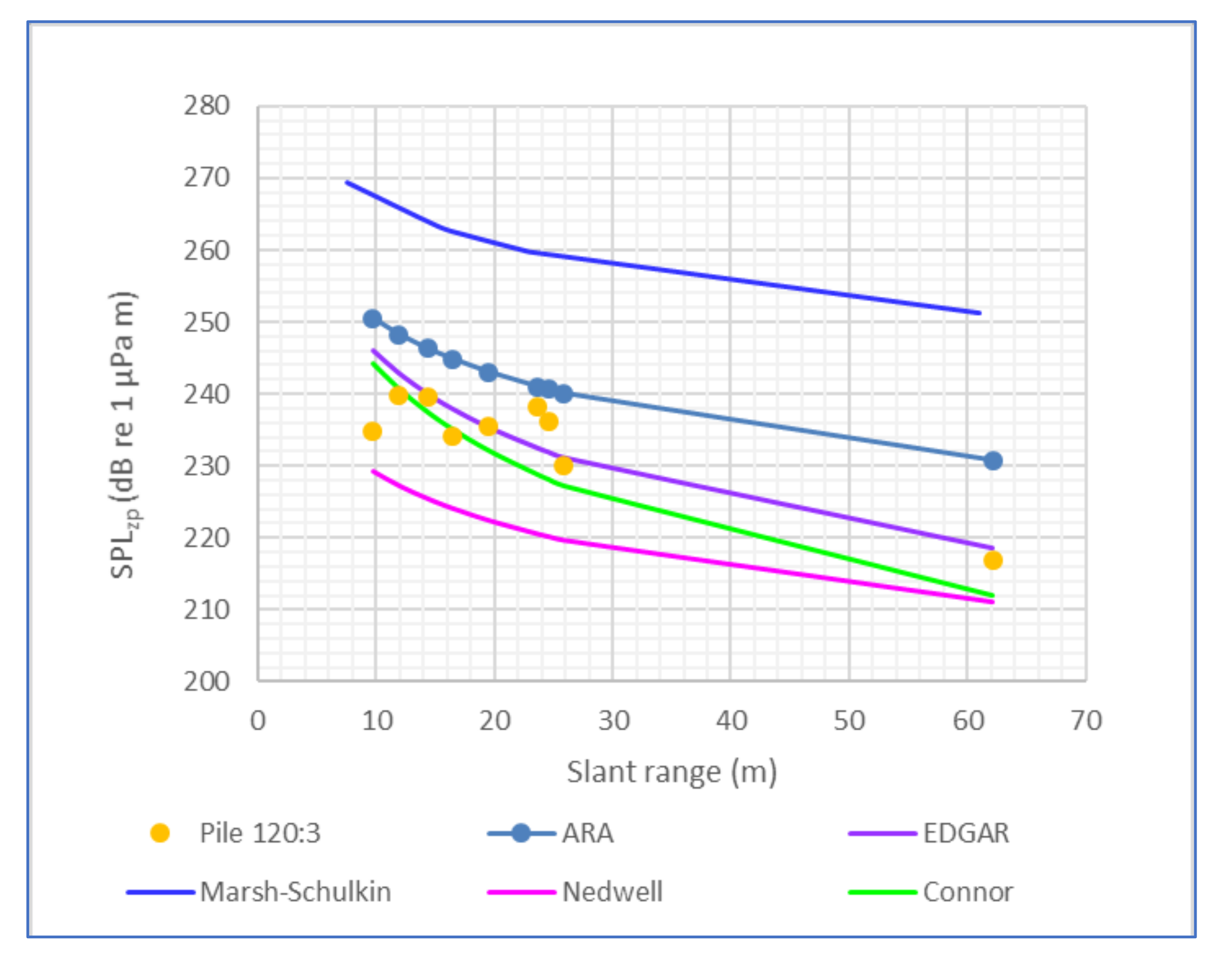
The EDGAR underwater noise model for $SP{L}_{pk}$ determination originated from a preliminary study made by the author, which compared the results of underwater sound propagation using the following models: ARA [9], Connor [6], EDGAR (current study), Marsh–Schulkin [22,23] and Nedwell [5] (Figure 2).

Basic observations concluded that SPL values were overestimated by the ARA [9] and Marsh–Schulkin [22,23] models and underestimated by Nedwell’s [5] model (Figure 2). Connor’s model gave reasonable estimates over short distances but underestimated the SPL as the distance increased (Figure 2). The Marsh–Schulkin open water model overestimated the impact radii about four-fold, when used with charges placed in metal tubes (piles or conductors) below the mudline (BML) (Figure 2).

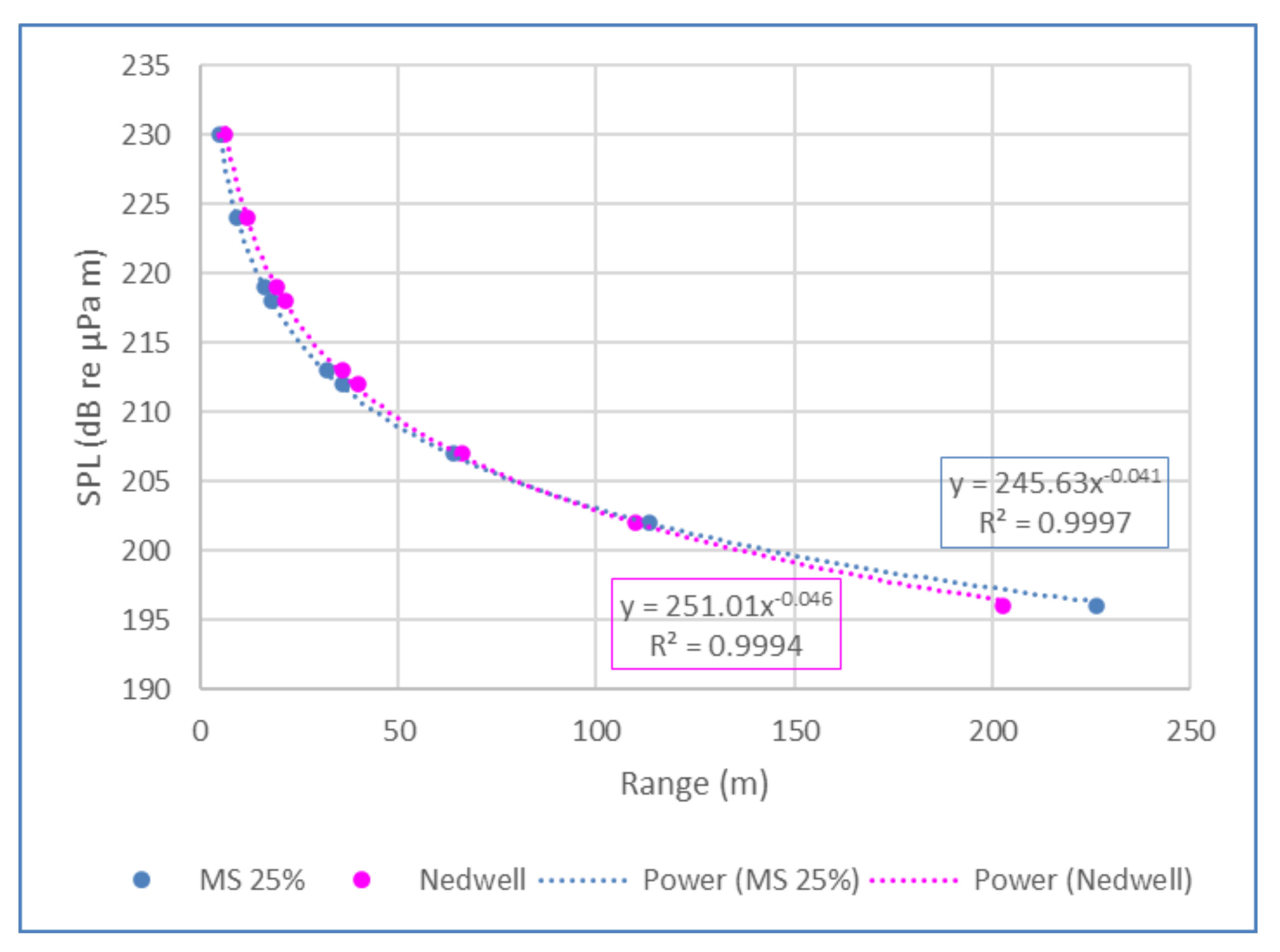
To investigate the existing models further, SPL_pk for a notional 1-kilogram TNT charge was plotted against a range (m) for a reduced (25%) Marsh–Schulkin model [22,23] and the Nedwell model for TNT charges embedded in boreholes (confined charges) [5] (Figure 3). As the Marsh–Schulkin model appeared to overestimate the impact radii about four-fold, the calculated range was reduced to a quarter of its value.

For Nedwell’s model, the parameter values used in Equation (2) were $K_p=2.55\times {10}^6$ for confined blasts, and $K_p=5.24\times {10}^7$ for open water blasts, with ${\alpha }_p=1.13$ for both scenarios [5]. It was noted that Nedwell’s model estimated the source level of the sound for confined charges (at 1 m) to be 248 dB re 1 μPa·m, which is approximately 11% less than the 279 dB re 1 μPa·m calculated using Equation (9).

Power relationships were fitted to the plots in Figure 3. It was observed that the power relationships were of the following form:

$$SP{L}_{pk}\approx S{L}_{pk}{r}^{-m_x/{10}^3}$$

(12)

where $SP{L}_{pk}$ is the peak SPL (in dB re 1 μPa·m), $S{L}_{pk}$ is the peak source level (in dB re 1 μPa·m), $r$ is the impact radius (m) and $m_x$ is a dimensionless gradient factor.

As $K_p$ and ${\alpha }_p$ in Equation (2) are empirical parameters that depend on the explosive type, their variability means that there is no simple consistent model with which SPL can be determined. Hence, if Equation (12) could be improved such that a gradient factor could be found to enable SPL_pk to be directly determined from the SL_pk, this would be an inherently useful breakthrough. Consequently, m_x was found using an iterative process that investigated values for the gradient factor ranging from 41 to 46, as in the power relationships given in Figure 3.

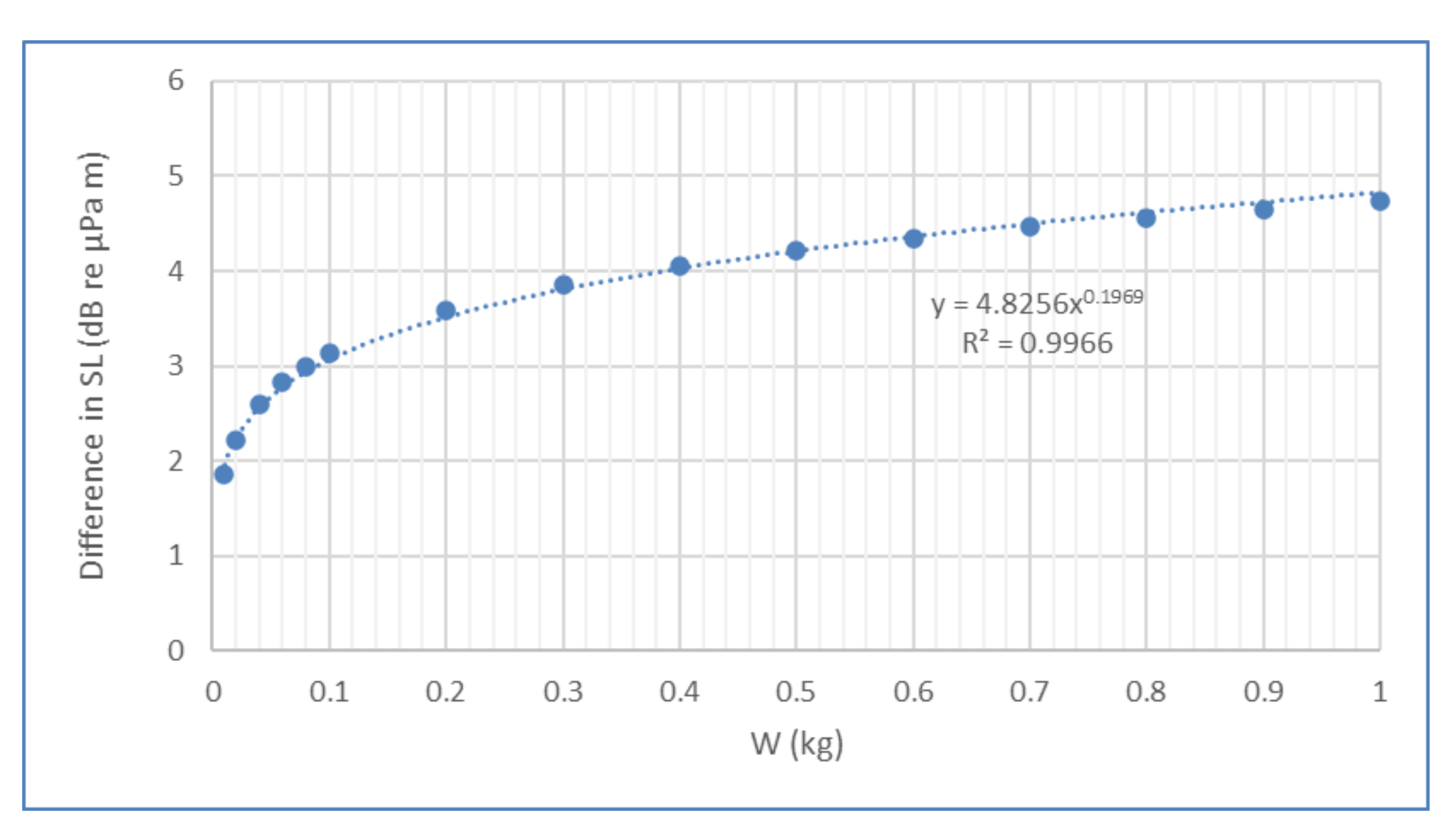
To optimise the model, an adjustment was made to the source level to minimise divergence from the other models when $r$ > 50 m. The divergence noted between the SL values calculated using Nedwell’s model for TNT charges embedded in boreholes ([5] Equation (2) with $K_p=2.55\times {10}^6$ and ${\alpha }_p=1.13$), and a 10% reduction in SL determined from Equation (9) was investigated for a range of charge weights (Figure 4).

In its final form, the EDGAR model for $SP{L}_{pk}$ is given by the following:

$$SP{L}_{pk}=\left\{\begin{array}{ll}\left(\frac{S{L}_{pk}+A_{ED}{W}^{b_{ED}/3}}{r^{m_x/{10}^3}}\right)& m_x=44,\mathrm{for}\mathrm{open}\mathrm{water}\\ \left(\frac{S{L}_{pk}+A_{ED}{W}^{b_{ED}}}{r^{m_x/{10}^3}}\right)& m_x=64,\mathrm{for}\mathrm{conductor}\mathrm{or}\mathrm{pile}\end{array}\right.$$

(13)

where $S{L}_{pk}$ is determined using Equation (9), the gradient factor $m_x$ is as given and $r$ is the slant range in m. The adjustment to the SL found in Figure 4 is given as $A_{ED}{W}^{b_{ED}}$ for pile and conductor severance, where $W$ is the charge weight in kg, and $A_{ED}$ = 4.8256 and $b_{ED}$ = 0.1969 are constants. Note that the divergence found between SLs for open water blasts was smaller and the adjustment is given by $A_{ED}{W}^{b_{ED}/3}$ Note that the slant range is used in EDGAR for the impact radius, rather than the radial range, as it is a more conservative measure. The slant range from the charge to the gauge is equivalent to the length of the hypotenuse of the triangle formed by the horizontal distance between the charge and each gauge line, and the vertical distance between the charge depth below the mudline and the height of each gauge above the mudline [6].

Additionally, the only inputs required for estimation of the $SP{L}_{pk}$ by EDGAR are the type of activity, and the weight and type of explosive charge (unadjusted for TNT-equivalence).

2.4. Model Assumptions

The marine environment is complex, and sound propagation can be affected in many ways [18].

• Geometrical and cylindrical spreading of sound away from its source
• Sound absorption by seawater and seabed
• Interactions with the

  o

  sea surface (reflection and scattering)

  o

  seabed (and transmission through)

• Refraction of sound
• Water depth and bathymetry between source and receiver
• Depth of source and receiver.

Several of the above factors depend on the acoustic frequency, and a complex model will include frequency dependence explicitly within the model parameters. However, many of the above factors are highly context dependent and, as such, many preclude a model from being used over a wide spatial extent.

As in TAP-118, the effects of bottom material were ignored because the first 1 to 2 m of bottom material in many parts of the ocean has a porosity of 60–80% [6]. The particle diameters of silty material and fine sand range from 1/16 to 1/256 mm and 1/4 to 1/8 mm, respectively. Thus, the shock from a severance detonation propagates through a largely water-like material, and the effect of the small solid particles was assumed to be negligible.

The procedure for measuring the sound generated from the use of explosives in TAP-118 [6] involved a number of unavoidable assumptions. These include the following:

Charge-to-gauge slant ranges are indefinite for the following reasons:

• Charge depths below the mud were uncertain (±45 cm);
• Surface float line curvature was estimated;
• Gauges were assumed to hang vertically, directly below their respective surface floats, which ignores the effects of subsurface currents;
• Gauge line-to-platform attachment points were chosen arbitrarily; and their exact locations were unknown for all shots;
• Tie line length to the first gauge line was uncertain (±1 m).

As a result of these ambiguities, the magnitude of the uncertainty in the charge-to-gauge slant ranges was estimated to be a minimum of 1.5 m.

Similar issues affected all the GOM projects.

2.5. Model Evaluation

Most mathematical models used for calculating variables or simulating processes in environmental sciences must be previously evaluated with techniques that allow for their performance assessment. This consists of an investigation of how well the model fits the data and whether outliers are present, the magnitude of any prediction errors and if the model is biased.

2.5.1. Goodness of Fit Indices

The correlation coefficient is a useful goodness-of-fit index; however, it is theoretically applicable only to linear models that include an intercept. Even for the commonly used power model, y = ax^b, the computed correlation coefficient can be a poor estimator of goodness of fit because of model bias. The correlation coefficient assumes that the model being tested is unbiased, that is, the sum of the errors is equal to zero and a fitted power model can be significantly biased [25].

Recognizing the limitations of the correlation coefficient, the Nash–Sutcliffe index, or the following efficiency index, $E_f$, can be used instead:

$$E_f=1-\frac{{{\displaystyle \sum }}_{i=1}^n{\left(P_i-O_i\right)}^2}{{{\displaystyle \sum }}_{i=1}^n{\left(O_i-\overline{O}\right)}^2}=1-{\left(\frac{\mathrm{RMSE}}{SD\left(O_i\right)}\right)}^2$$

(14)

where $P_i$ and $O_i$ are the predicted and measured values of the dependent variable, respectively; $\overline{O}$ and $SD\left(O_i\right)$ are the mean and the standard deviation of the measured values, respectively; RMSE is the root mean squared error; and $n$ is the sample size. If the predictions of a linear model are unbiased, then the efficiency index will lie in the interval from 0 to +1. For biased models, $E_f$ may be algebraically negative, which suggests that the mean of the observed values is a better predictor than the evaluated model [26]. For nonlinear models, negative efficiencies can result even when the model is unbiased.

According to McCuen et al. [25], the $E_f$ may be a useful goodness-of-fit indicator, but its limitations should be taken into account. It is a single-valued index that can be sensitive to several factors, including sample size, outliers and bias. Failure to recognize the limitations of $E_f$ may lead to rejection of a good model solely because $E_f$ was misapplied, such as to a biased model.

2.5.2. Quantification of Prediction Errors

The Root Mean Squared Error (RMSE) measures the average magnitude of the error in terms of the units of the variable calculated by a model.

$$\mathrm{RMSE}=\sqrt{\frac{1}{n}{\displaystyle \sum }_{i=1}^n{\left(P_i-O_i\right)}^2}$$

(15)

where $n$ is the sample size, and $P_i$ and $O_i$ are the predicted and measured values. It ranges from 0 to ∞, where RMSE $=0$ indicates a perfect fit. Since the errors are squared before they are averaged, the RMSE gives a relatively high weight to large errors.

The Mean Absolute Error (MAE) measures the average magnitude of the errors in a set of predictions, without considering their direction.

$$\mathrm{MAE}=\frac{1}{n}{\displaystyle \sum }_{i=1}^n\left|P_i-O_i\right|$$

(16)

Both MAE and RMSE express an average model prediction error in units of the variable of interest. Both metrics can range from 0 to ∞ and are indifferent to the direction of errors. They are negatively oriented scores, which means lower values are better.

MAE can be used to define bounds for the RMSE, as $\mathrm{MAE}\le \mathrm{RMSE}\le \sqrt{n} \mathrm{MAE}$ [27]. The upper bound, $\sqrt{n} \mathrm{MAE}$, suggests that the RMSE tends to become increasingly larger than the MAE as the test sample size increases. This can be problematic when comparing RMSE results calculated on different sized test samples.

Note that the above measures will have the same units as the variable to be predicted and thus, cannot be compared for different variables that are scaled differently. The error can be normalised using the ratio of the RMSE to the standard deviation of the measured data to give the Normalised Root Mean Squared Error (NRMSE) [27],

$$\mathrm{NRMSE}=\frac{\mathrm{RMSE}}{SD\left(O_i\right)}=\sqrt{\frac{{{\displaystyle \sum }}_{i=1}^n{\left(P_i-O_i\right)}^2}{{{\displaystyle \sum }}_{i=1}^n{\left(O_i-\overline{O}\right)}^2}}$$

(17)

The NRMSE includes a scaling/normalisation factor; therefore, the resulting statistic and reported values can apply to various constituents [28]. NRMSE varies from the optimal value of 0, which indicates zero RMSE or residual variation and, therefore, a perfect model simulation, to a large positive value. The lower the NRMSE is, the lower the RMSE is, and the better the model simulation performance is, with RMSE values less than 0.5 SD of the measured values being considered low [28]. Hence, a model run with an NRMSE of less than 0.5 was considered to have performed “very well”. Two other performance ratings of “well” (0.5 < NRMSE ≤ 0.6) and “acceptable” (0.6 < NRMSE ≤ 0.7) were also adopted.

2.5.3. Bias

Environmental science models do not perfectly replicate measured data, with the error variation reflecting the potential prediction accuracy, or inaccuracy, of the model. The error variation in the predicted values of a random variable can be due to both systematic and non-systematic causes. Systematic error variation is referred to as a bias, with a positive bias indicating overprediction.

Power models are often biased when calibrated using logarithms [25]. Model bias is estimated using the average error, where an error is the difference between the predicted and measured values. The bias, $\overline{e}$, has the same units as the dependent variable and is computed by

$$\overline{e}=\frac{1}{n}{\displaystyle \sum }_{i=1}^n\left(P_i-O_i\right)$$

(18)

where $n$ is the sample size, and $P_i$ and $O_i$ are the predicted and measured values of the dependent variable, respectively. A bias is more easily interpreted when it is stated in relative terms ($R_b$), which is the ratio of the bias to the mean of the measured values.

$$R_b=\frac{\overline{e}}{\overline{O}}$$

(19)

$R_b$ is dimensionless and takes the sign of $\overline{e}$. A relative bias greater than 5% in absolute value may be considered significant [25]. Positive values indicate model overestimation bias, and negative values indicate model underestimation bias [28].

It is always important to report the bias and relative bias along with the efficiency index, $E_f$.

2.5.4. Outliers

In this study, outliers were those observation–simulation pairs with a difference that is greater than three standard deviations. Outliers were removed from the data set before model development.

Sources of model error were also examined using graphical plots.

2.6. Underwater Noise Data for Model Evaluation

In the GOM TAP projects and OCS studies, cutting charges were placed within piles and/or conductors at varying depths BML to gather the following in situ blast effect data: peak pressure, impulse and acoustic energy [1,6,7,17,24]. Acoustic receivers (transducers) were arranged in an array, along near-field and far-field downlines placed at set distances from a target structure [1,6,7,17,24].

Table 1. Gulf of Mexico decommissioning projects using explosive severance.

Project No.	Project Title	Reference
TAP-025	Overpressures Developed by Shaped Explosive Charges Used to Remove Wellheads	[7]
TAP-118	Blast Effects Upon the Environment from the Removal of Platform Legs by Explosives	[6]
TAP-429	Oil Platform Removal Using Engineered Charges: In Situ Comparison of Engineered and Bulk Explosive Charges	[24]
TAP-570	Measurement of the Effect of Depth Below Mudline of Charge Placement During EROs	[1]
OCS Study MMS 2003-059	Shock Wave/Sound Propagation Modeling Results for Calculating Marine Protected Species Impact Zones During Explosive Removal of Offshore Structures	[9]
OCS Study MMS 2005-013	Structure-Removal Operations on the Gulf of Mexico Outer Continental Shelf	[29]
OCS Study BOEM 2016-019	Pressure Wave and Acoustic Properties Generated by the Explosive Removal of Offshore Structures in the Gulf of Mexico	[17]

Note: Technology Assessment Program (TAP) Projects were previously known as Technology Assessment Research (TAR) Projects before the creation of the Bureau of Safety and Environmental Enforcement (BSEE).

lists the GOM projects that were used in the current study as sources of data and models.

Further details of the GOM TAP projects and OCS studies are given in the Appendix A: (Table A1).

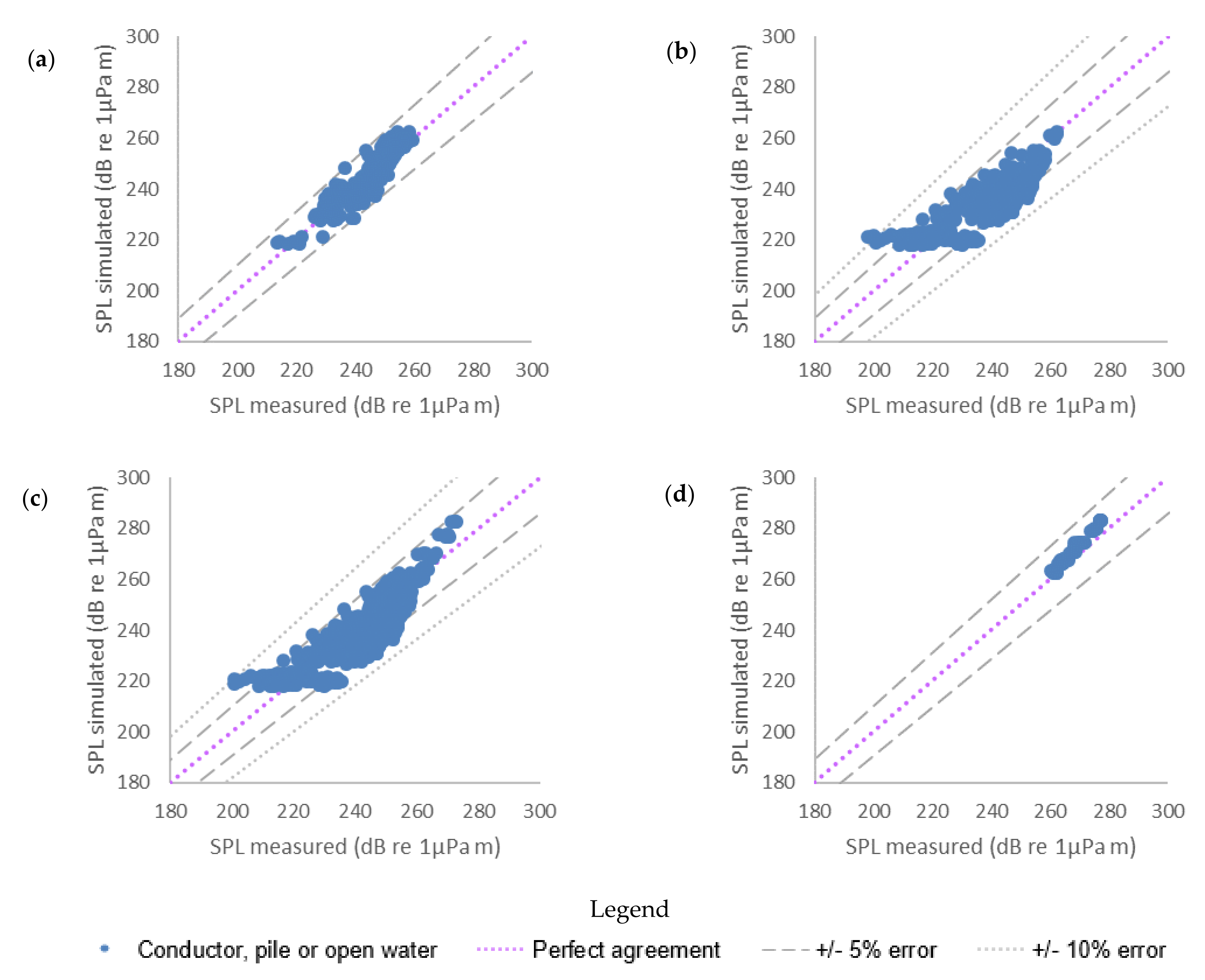
3. Results and Discussion

The simulated and measured values of SPL_pk for explosive conductor/pile severance and open water blasts were highly associated (

Table 2. Statistical evaluation of EDGAR simulated values and measured Gulf of Mexico TAP-118 project data for conductor and pile severance BML. Main and skirt piles were air- and water-terminated, respectively. Adj R²: adjusted coefficient of determination; MAE: mean absolute error; RMSE: root mean squared error; and NRMSE: normalised root mean squared error.

Severance Type	r	Adj R2	Lower Bound (=MAE) (dB re 1 µPa·m)	RMSE (dB re 1 µPa·m)	$\mathbf{Upper}\mathbf{Bound}(=\sqrt{\mathit{n}}\mathbf{MAE})$ (dB re 1 µPa·m)	RMSE (%)	Nash–Sutcliffe Efficiency Index, Ef	NRMSE	Bias (dB re 1 µPa·m)	Relative Bias (%)	n
Conductor	0.93	0.86	2.89	3.55	21.64	1.51	0.85	0.38	−0.55	−0.23	56
Main/leg pile	0.95	0.89	3.64	4.45	31.98	1.88	0.89	0.34	−0.31	−0.13	77
Skirt pile	0.78	0.60	5.82	7.25	46.94	3.14	0.56	0.66	−2.15	−0.93	65

Source: TAP-118 [6].

and

Table 3. Statistical evaluation of EDGAR simulated values and measured Gulf of Mexico project data for combined conductor, pile and conductor/pile severance BML and for open water blasts. Adj R²: adjusted coefficient of determination; MAE: mean absolute error; RMSE: root mean squared error; and NRMSE: normalised root mean squared error.

Severance Type	r	Adj R2	Lower Bound (=MAE) (dB re 1 µPa·m)	RMSE (dB re 1 µPa·m)	$\mathbf{Upper}\mathbf{Bound}(=\sqrt{\mathit{n}}\mathbf{MAE})$ (dB re 1 µPa·m)	RMSE (%)	Nash–Sutcliffe Efficiency Index, Ef	NRMSE	Bias (dB re 1 µPa·m)	Relative Bias (%)	n
Conductor (BML)	0.90	0.81	3.48	4.35	47.19	1.79	0.77	0.48	−0.17	−0.07	184
Conductor & Pile	0.89	0.79	5.25	6.69	126.36	2.78	0.78	0.47	−1.03	−0.43	597
Pile	0.85	0.73	6.60	8.10	122.36	3.44	0.69	0.56	−1.94	−0.82	344
Openwater	0.99	0.98	3.57	3.86	29.02	1.44	0.38	0.79	3.57	1.34	66

Note: Conductor (BML) refers only to conductors where the explosive charge was placed below the mudline. Sources: TAP-025 [7]; TAP-118 [6]; TAP-570 [1]; BOEM 2016-019 [17].

), suggesting that the trends in measured values are well simulated. The correlation coefficient between the simulated and measured values for all of the scenarios is highly statistically significant (p < 0.0001), with r varying from 0.78 to 0.95 for pile severance, and 0.90 to 0.93 for conductor severance (Table 2 and Table 3). The combined conductor/pile severance and the open water blast had r values of 0.89 and 0.99, respectively (Table 3).

All the conductor and pile severance simulations showed acceptable absolute relative biases of less than 1%, whilst the relative bias for open water blasts was 1.34% (Table 2 and Table 3). The relative biases of all the severance SPLs for TAP-118 and combined severance simulations were negative, suggesting a small systematic underestimation, whereas EDGAR slightly overestimated the SPLs of the open water blasts.

All the scenarios displayed coincidence with total errors close to the lower RMSE bounds and acceptable RMSEs of less than 3.5% (Table 2 and Table 3).

The best performing models with efficiency indices of >0.75 and NRMSEs of 0.5 or less were TAP-118 conductors and main piles (Table 2) and all combined conductors and conductors/piles (Table 3). The combined pile model performed well (0.5 < NRMSE ≤ 0.6; 0.65 < E_f ≤ 0.75) (Table 3), and the TAP-118 skirt pile model’s performance was acceptable (0.6 < NRMSE ≤ 0.7; 0.5 < E_f ≤ 0.65) (Table 2). Using the same metrics, the performance of the open water blast model was deemed unsatisfactory. However, the near perfect association (r = 0.99) and low relative bias (1.34%) of the open water blast model suggests merely that it consistently overestimated the SPL, and that it is a conservative model (Table 3). The bias of the latter model is 3.57 dB re 1 μPa·m, which represents an approximate overestimation of 50% in the sound pressure.

Note that the model performed better for air-terminated main piles than for water-terminated skirt piles (Table 2). However, whilst the skirt pile data likely influenced the model performance for combined piles and conductors/piles, compared to combined conductors (as indicated by the increase in RMSE and NRMSE, bias and relative bias), EDGAR still performs very well for combined conductors/piles. Connor [6] suggested that sound pressure values were indistinguishable between water-terminated and air-vented conductors. He also noted that there was no difference between the pressure pulses observed with charges detonated at different depths BML near either the main or skirt piles.

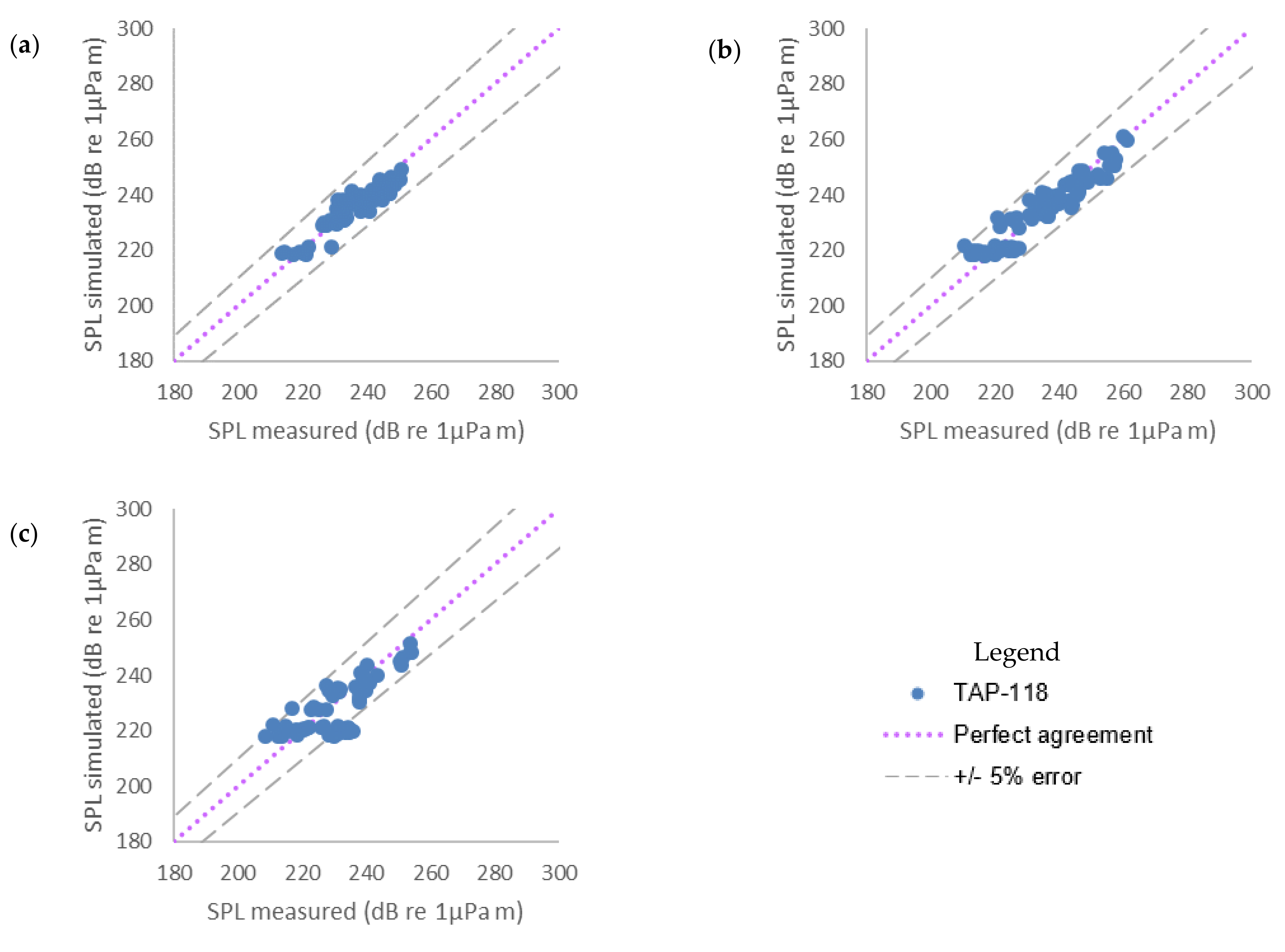
The simulated SPLs were plotted against measured values from the TAP-118 project [6] (Figure 5) and data from several GOM projects combined (TAP-025 [7], TAP-118 [6]; TAP-570 [1] and BOEM 2016-019 [17]) (Figure 6). The 1:1 lines, which represent perfect agreement between the simulations and the measurements, are shown on the plots. The spread of points around the 1:1 line indicates the errors in the simulations of SPLs compared to the measurements. Figure 5 shows that the majority of simulations were within ±5% of the measured values for TAP-118 data [6]. This is also true for the combined conductors and open water blasts (Figure 6a,d, respectively), whilst all the simulations are within ±10% (Figure 6).

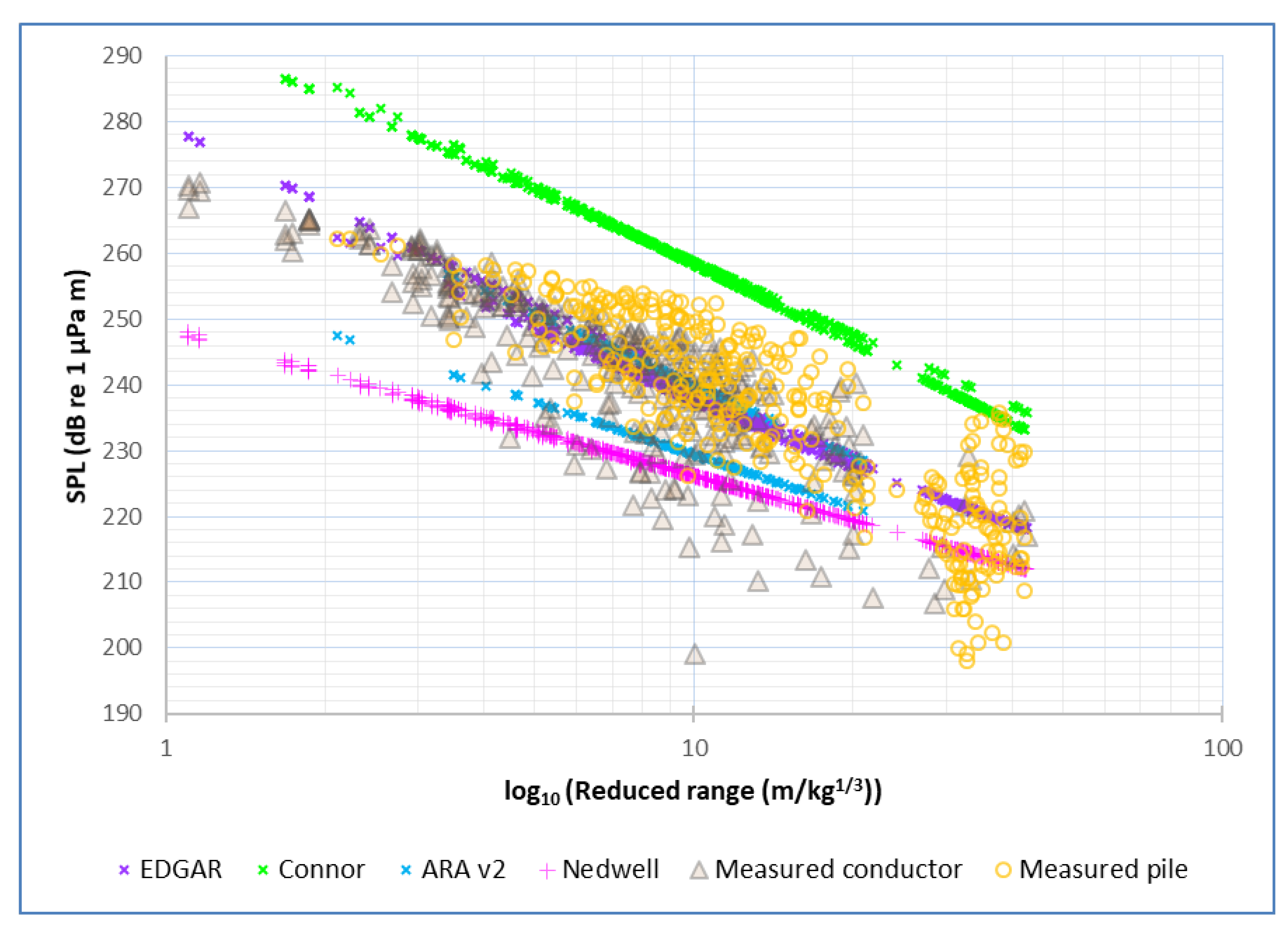
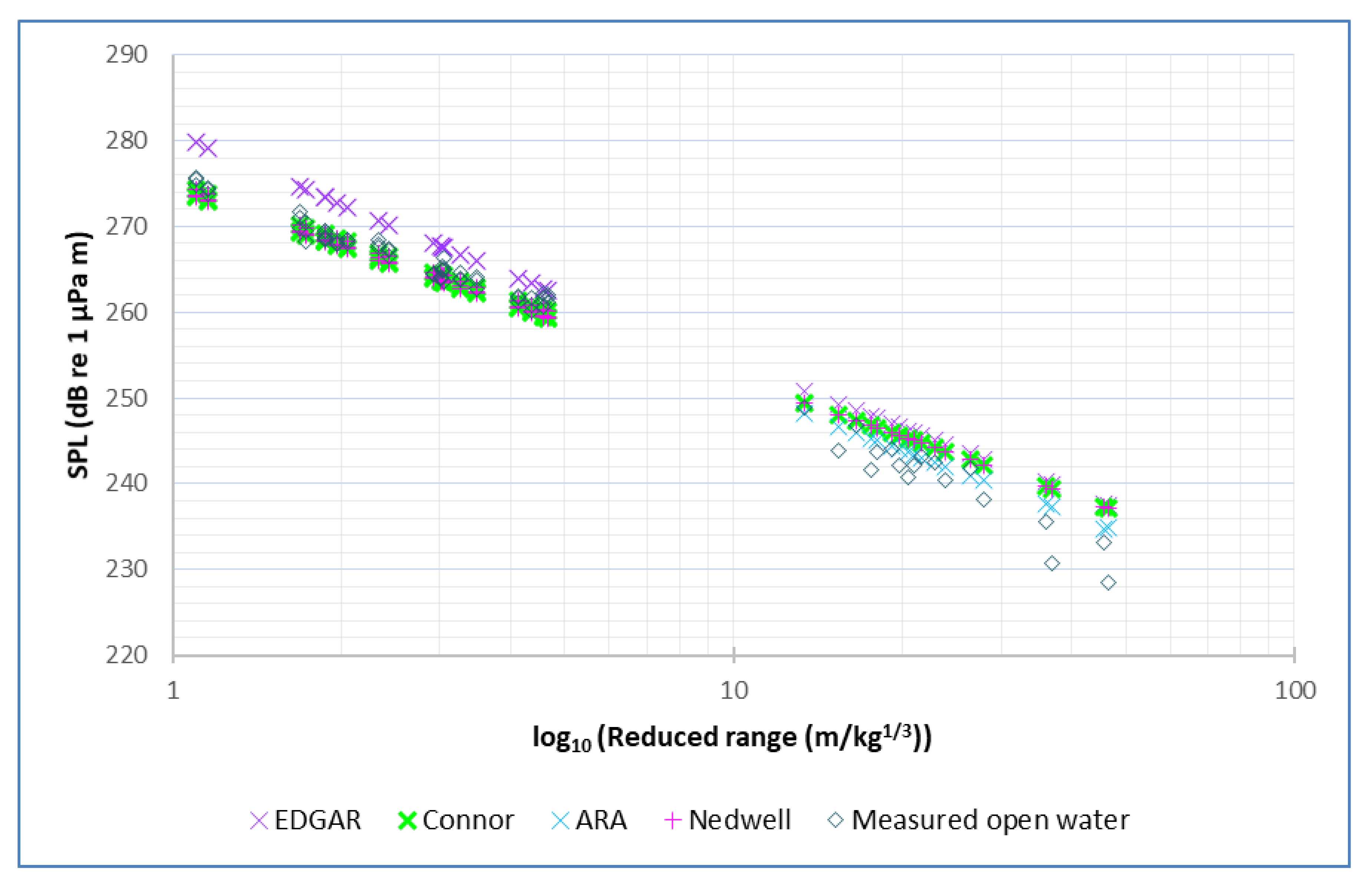
Simulated and measured SPL values were plotted against the log of the reduced range (${\log }_{10}\left(r/W^{1/3}\right)$) (Figure 7: explosive severance BML and Figure 8: open water blasts). Simulated values were modelled using EDGAR, ARAv2 [9], Connor [6] and Nedwell [5]. The Nedwell model tends to underestimate SPLs, whilst Connor’s model overestimates them (Figure 7). At first observation, ARAv2 appears to give a good fit with distinct estimates for piles and conductors (Figure 7). However, the upper and lower blue lines represent conductor and pile severance, respectively, whilst the measured data shows that pile severance SPL values are generally higher than for conductors. EDGAR is similar to the ARAv2 conductor model for all the severance operations (Figure 7).

Figure 8 illustrates that EDGAR consistently overestimates open water blast SPLs. Connor’s, Nedwell’s and the ARAv2 models initially underestimate SPLs at low reduced ranges but tend to overestimate SPLs with an increasing range.

The measured GOM project data displayed in Figure 7 were highly variable and the reasons for this have been discussed in detail in the individual GOM project reports [1,6,7,9,17,24,29]. Piles were observed to have been severed to different degrees [29]. Barkaszi et al. [17] suggested that anomalous data points, which came from the near-bottom sensors, resulted from the interaction of pressure waves (direct or reflected from the substrate). Connor [6] noted that although care was taken to avoid mounting gauges in the cavitation layer just below the air/water interface, one gauge produced pressure values significantly lower than the values observed at the surrounding gauges. This was attributed to the gauge potentially being in the lower portion of the cavitation layer.

If the charge energy is directly and perfectly coupled to the conductor/pile, the efficiency, that is the ability for a medium to conduct and transmit sound waves is maximized [1]. Charge energy will be reduced where cavities exist between the charge and item to be severed, as these will fill with water, air or mud. The numerical simulations performed by Dzwilewski et al. [9] indicated that some energy loss is due to explosive energy propagating in the water inside the pile (typically less than 5%).

For well conductors, issues arise regarding the number and size of inner well casings, the presence (or lack of) and type of grouting and other structural anomalies. Poe et al. [1] suggested that some of the variables that influence coupling efficiency are as follows:

• Bulk versus shaped charge and the configuration of each;
• Physical coupling between the charge and pile/jacket;
• Distance below mudline: this changes the effective local impedance of the pile;
• Depth of jetting in pile below the charge location; and
• Amount of water/air in the pile/jacket.

The coupling between the pile and seabed also influences efficiency. Dzwilewski et al. [9] simulated explosive coupling efficiencies for stiff clay (79%), a pile in water (49%) and a pile in clay (39%). They noted that multiplication of the first two efficiencies, stiff clay by pile in water gives the efficiency for the combined pile in clay. The simulations showed that a reduction in coupled energy into the water was dominated by the high strength and density of the pile and soil confinement. Further, more energy is coupled into water for thinner pile walls, larger pile diameters and higher explosive weights.

In addition, the actual composition of the local seabed will further determine the efficiency. Softer sediments will attenuate acoustic and pressure waves more effectively than harder sediments. Barkaszi et al. [17] suggested that the liquefied nature of the sediments found in the BOEM 2016-019 sites may contribute to the inconsistency of the linear attenuation of the pressure wave. However, they noted that it was not possible to quantify the specific contribution from suspended particles, water depth, structural interference or other controlling factors, such as gas bubble entrapment. There is likely a synergistic effect among multiple factors that results in complex attenuation patterns in the near field.

4. Conclusions

A simple, but dynamic, underwater noise model driven by only simple, minimal input data has been described and estimates of the underwater noise generated during explosive activities evaluated. This model will be easily adaptable for different uses by other researchers as it is highly transparent, on account of being written in Excel, and is documented in detail. Different modules could easily be incorporated, allowing the functionality of the rest the model to be used with any new additions.

A sound propagation model should be fit for purpose and suited to the task at hand. EDGAR has been benchmarked against historical Gulf of Mexico data and compared with other decommissioning underwater noise propagation models designed for use with explosives. EDGAR provides a good fit to the Gulf of Mexico measured data over the range of distances from the sources for which measurements are available.

Many underwater noise models are complex multiparameter models, some of which may only be valid in limited environmental settings. EDGAR is an easy-to-use quick reference tool to aid industry and regulators alike to make decisions about the environmental impacts of decommissioning.

EDGAR provides a fit-for-purpose tool that can be used by government regulators and their advisers, oil and gas operators and environmental consultancies, to understand the impact of underwater noise from explosives use on marine species, especially marine mammals. This could help industries access the sciences, reducing consultancy, regulator and operator decommissioning costs.

In the future, EDGAR may be expanded to include the impact of unexploded ordnance on marine mammals and fish during wind farm development.