Article

Development of a Framework for Wind Turbine Design and Optimization

by
Mareike Leimeister
1,*,
Athanasios Kolios
2 and
Maurizio Collu
2
1
Fraunhofer Institute for Wind Energy Systems IWES, Am Luneort 100, 27572 Bremerhaven, Germany
2
Naval Architecture, Ocean and Marine Engineering, University of Strathclyde, Glasgow G4 0LZ, UK
*
Author to whom correspondence should be addressed.
Modelling 2021, 2(1), 105-128; https://doi.org/10.3390/modelling2010006
Submission received: 25 January 2021 / Revised: 8 February 2021 / Accepted: 9 February 2021 / Published: 16 February 2021
(This article belongs to the Section Modelling in Engineering Structures)

Abstract

:
Dimensioning and assessment of a specific wind turbine imply iterative steps for design optimization, as well as load calculations and performance analyses of the system in various environmental conditions. However, due to the complexity of wind turbine systems, fully coupled aero-hydro-servo-elastic codes are indispensable to represent and simulate the non-linear system behavior. To cope with the large number of simulations to be performed during the design process of a wind turbine system, automation of simulation executions and optimization procedures are required. In this paper, such a holistic simulation and optimization framework is presented, by which means iterative simulations within the wind turbine design assessment and development processes can be managed and executed in an automated and high-performance manner. The focus lies on the application to design load case simulations, as well as the realization of automated optimizations. The proper functioning and the high flexibility of the framework tool is shown based on three exemplary optimization tasks.

1. Introduction

Wind turbines have to withstand various loadings—static and dynamic, structural and environmental. Besides wind loads on any wind turbine, offshore systems also have to deal with environmental impact from waves, currents, tides, and sea ice. These external factors place high demands on the design of a wind turbine system, while also other requirements related to costs, manufacturing, size, performance, and system safety have to be met. This makes the development of wind turbines a highly iterative process, in which the design needs to be optimized and assessed.
Standards, such as IEC 61400-3-1 [1] and IEC TS 61400-3-2 [2] or DNVGL-ST-0437 [3], describe design load cases (DLCs), which are grouped into normal, fault, and other—transport or installation—design situations. DLCs are used to asses ultimate and fatigue loads on the system and, this way, to approve the system integrity and to show that the wind turbine can withstand all prevailing environmental conditions during its design life. Considering various normal and extreme conditions for the different design situations leads to a huge set of load cases, for which prescribed parameters have to be set. For this application an automated simulation framework is required.
Furthermore, to support the development of a wind turbine design through an optimization process, iterative simulations have to be executed. In these, a number of design variables have to be modified until an appropriate design, optimized with respect to a range of prescribed criteria, is achieved. However, due to the complexity of wind turbine systems, as well as their non-linear and fully coupled aero-hydro-servo-elastic behavior, this optimum solution has to be derived through modeling and simulation. Therefore, a framework for automated optimization of wind turbine systems is essential.
A huge variety of optimization methods is available and finds application to optimization tasks for the complex engineering systems in the field of renewable energies [4,5]. In the particular case of wind turbine systems, not only the optimization approaches, but also the optimization objectives are multifaceted. Apart from the most common and overall goal of reducing the system costs or levelized cost of energy, as well as maximizing the annual energy production [6,7,8,9,10,11,12,13,14,15,16,17,18,19,20,21,22,23,24], the optimization focus also often lies on the loads on the system, including fatigue [6,10,11,12,14,15,21,25,26], as well as the dynamic system response [11,12,14,22,27]. The component of interest, which is to be optimized, ranges from the blades [15,19,20,21,23,24,26,28,29], the control system [24], the tower [10,13,15,19,20,23,24], and the support structure [10,25,27], which might even be floating [6,11,12,14,27,30], to the mooring lines and power cable [14], and even to wind farms, which might be optimized with respect to their location, layout, or utilized turbines [7,8,9,16,17,18]. The optimization itself can be done analytically and gradient-based [15,25,27]; however, most commonly evolutionary and genetic algorithms are applied [6,7,8,9,13,21,29]. Furthermore, due to the high complexity of wind turbine systems, simplified models, such as multibody or reduced-order models, are utilized for the application to optimization tasks [6,11,12,14,28,30]. Even in the already quite established field of wind farm design and layout optimization, the single wind turbine system is extremely simplified, as the main emphasis is on the farm economics and not on the fully coupled system dynamics of each single wind turbine within the farm.
The presented literature shows the need and relevance of design optimization methods for wind turbine systems. While the available optimization methods are mostly tailored to the specific optimization task and component of interest, there are also some multidisciplinary and integrated approaches, which focus on more than just one system component but mostly deal with aero-structural optimization [10,14,15,19,20,21,22,23,24,26,28,29]. The focus on specific components and optimization objectives is still present and reflected as well by the manner, in which the system is implemented: Simplified and reduced-order models for the wind turbine system are utilized [6,11,12,28,30], as well as aero-, hydro-, control, and structural dynamics are only selectively and/or just rudimentary represented [13,14,27]. Each method presented in the literature is valuable but limited to certain optimization problems. Thus, a holistic approach for optimization of wind turbine systems, which:
  • involves all system components, as well as their fully coupled aero-hydro-servo-elastic behavior;
  • is based on scientific fundamentals without the need for approximations;
  • uses systematic methods;
  • can potentially be extended to any level of detail and used for any optimization problem,
is the next development step and level of wind turbine design and optimization. Such a holistic and highly flexible optimization framework is developed and presented in this work. This framework is not only suitable for systematic optimization of wind turbine systems, but also for automated execution of simulations and optimization tasks. Furthermore, it implies fully coupled simulations of any wind turbine system—even floating.
Thus, this paper aims to present a novel engineering method for a fully flexible optimization approach by developing a fully modular, high-fidelity optimization approach, which is due to its modular character highly flexible and adaptable with respect to the application case, optimization problem, considered system, and level of detail. Hence, this work addresses the complex development process of engineering systems, implying advanced optimizations and iterative simulations (also in case of DLC simulations). The presented framework is very flexible and multifunctional and can be applied to wind turbine systems by utilizing Fraunhofer’s in-house tool MoWiT (Modelica® library for Wind Turbines), formerly OneWind Modelica® library, but also to other complex engineering systems when taking other Modelica® libraries as basis. The advantage of using Modelica®—based models within the framework is the high flexibility in the specific system of interest, as—due to the multibody approach and hierarchical structure in Modelica®—components can easily be exchanged and modified and, thus, any state-of-the-art onshore or offshore, bottom-fixed or floating wind turbine system can be realized [31]. The framework consists as well of an external programming framework. This structure allows the use of highly sophisticated optimization tools, so that various optimization tasks, as well as multi-objective problems, can be addressed. However, in addition to optimizations, the presented framework can also be employed for automated execution of simulations, which is for example very useful for dealing with the large number of DLCs recommended by the standards. The proper functioning and high flexibility of the presented framework tool is demonstrated through its application to three different optimization tasks.
The structure of this paper is the following: First, a generic description of such a framework for automated wind turbine system simulation is presented in Section 2. The application of this framework to automated DLC simulations is shown afterwards in Section 3. To cope also with optimization tasks, additional features need to be considered and incorporated in the framework (Section 4). Three examples for the application of the framework to optimization problems are presented in Section 5, while future developments are outlined in Section 6. Finally, conclusions are given in Section 7.

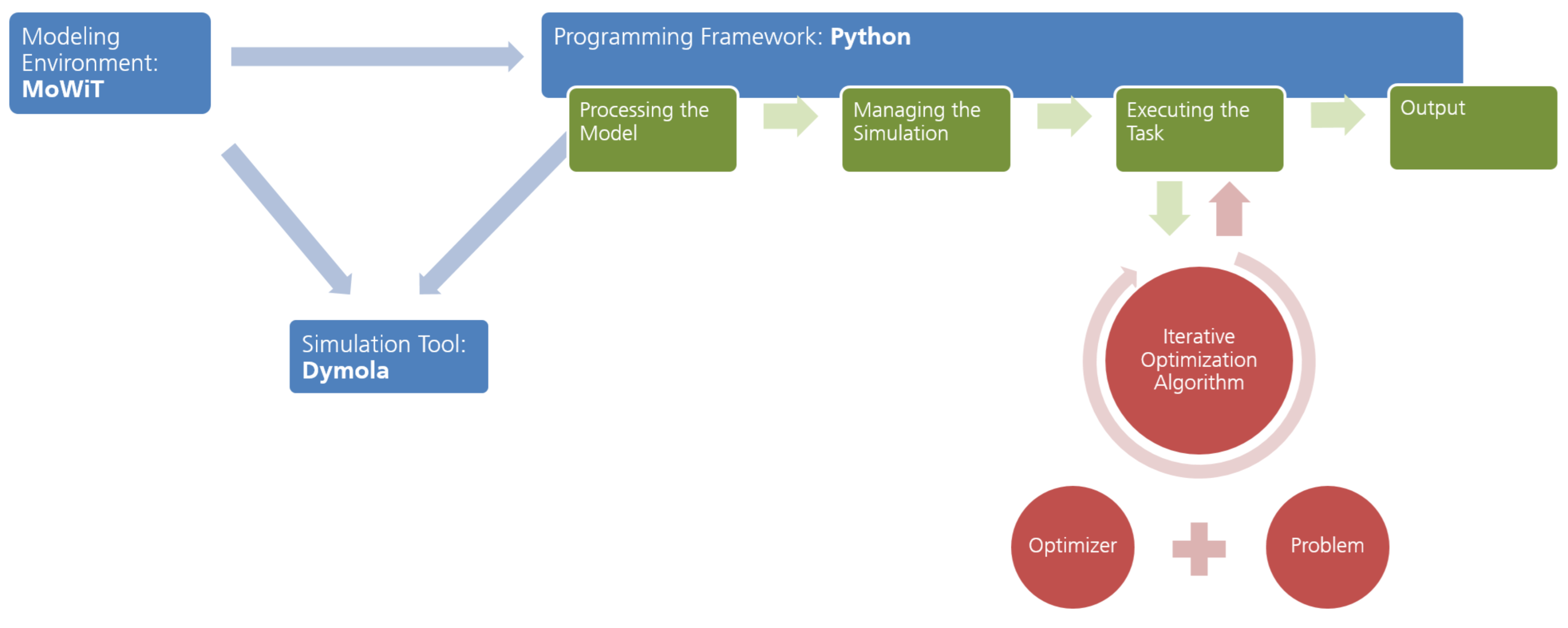
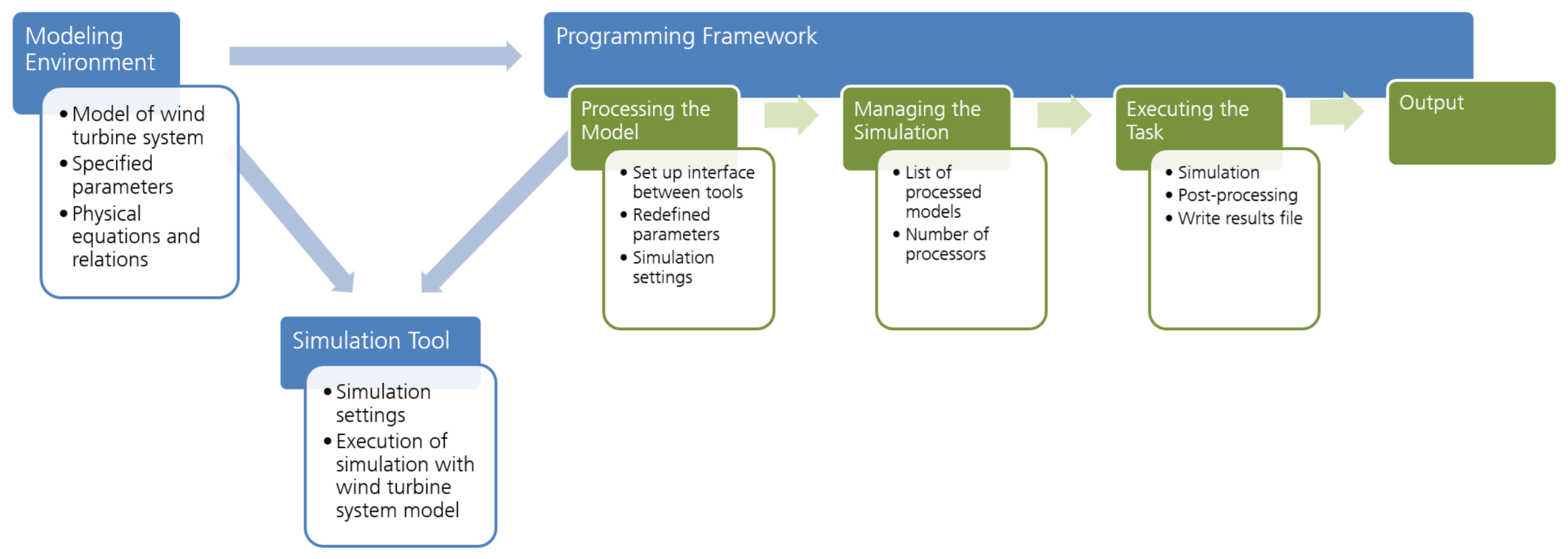
2. Framework for Automated Simulation

To establish such a framework for automated simulation of wind turbine systems, three main components, as presented in Figure 1 and described hereafter, are considered to be required. This modular structure allows the utilization of unique modules, which are sophisticated for the particular application.

2.1. Modeling Environment

First, there is the need for a modeling environment which is capable of representing the non-linear and fully coupled aero-hydro-servo-elastic behavior of an onshore or offshore wind turbine system, which might be in the latter case bottom-fixed or even floating. Within the model, all components of the system, corresponding parameters and variables, as well as their physical relations and the systems of equations, have to be specified.
Various codes and tools for wind turbine modeling, load calculation, and fully coupled aero-hydro-servo-elastic simulation are already developed, such as:
  • Bladed (https://www.dnvgl.com/energy/generation/software/bladed/index.html, accessed on 12 November 2018) by DNV GL, which is a wind turbine design and simulation software, by which means both the wind turbine and its environment can be modeled [32];
  • FAST (https://nwtc.nrel.gov/FAST, accessed on 12 November 2018) (Fatigue, Aerodynamics, Structures, and Turbulence) by NREL (National Renewable Energy Laboratory), which is an aero-elastic simulation tool for horizontal axis wind turbines, based on a code containing models for aero-, hydro-, control, and structural dynamics [33];
  • HAWC2 (http://www.hawc2.dk/, accessed on 12 November 2018) (Horizontal Axis Wind turbine simulation Code 2nd generation) developed at Risø National Laboratory in Denmark, which is an aero-elastic code for wind turbine design and load simulation and covers various models for dealing with aero-, hydro-, control, and structural dynamics [34];
  • MoWiT developed at Fraunhofer IWES (Institute for Wind Energy Systems) in Bremerhaven, Germany, which is a library based on the open-source object-oriented and equation-based modeling language Modelica® (https://www.modelica.org/, accessed on 2 October 2019) and by which means the entire wind turbine system can be represented through models for each single component, including the environment and aero-hydro-servo-elastic dynamics [35,36,37].
In this work, MoWiT, which is available free of charge for academic use, is selected as modeling environment due to its beneficial properties:
  • High flexibility
    Due to the object-oriented and equation-based modeling language Modelica®, its hierarchical programming structure, and its multibody approach, the complex wind turbine system can be represented through component-based computational models. Thus, MoWiT contains six main components (rotor, nacelle, operating control, support structure, wind, and waves), which comprise further subcomponents, such as the hub and blades within the rotor component, the drivetrain and generator within the nacelle component, or within the support structure component the tower, substructure, as well as ballast and mooring lines in case of a floating system. The single components and models are interconnected to represent the fully coupled aero-hydro-servo-elastic behavior of wind turbine systems. By adapting or exchanging single components, any state-of-the-art wind turbine system type (onshore or offshore, bottom-fixed or floating), various environmental conditions, and different simulation settings can be modeled.
  • Continuous enhancement and extension
    MoWiT is developed by engineers at Fraunhofer IWES. This allows continuous enhancement and extension of the library, including also verification and validation of the code [35,38,39,40,41]. Thus, different theories and approaches are implemented to represent the aero-hydro-servo-elastic dynamics of a wind turbine system and the degree of detail is refined on and on. The current capability of the in-house tool MoWiT is as follows [35,36,37,40]:
    -
    The blade-element-momentum theory with dynamic stall and dynamic wake, or the generalized dynamic wake model with dynamic stall, or stochastic wind and gust models can be utilized to represent unsteady aerodynamics.
    -
    The hydrodynamic loads due to regular or irregular waves can be determined based on the Morison equation or the MacCamy–Fuchs approach, with having different wave theories (linear Airy or non-linear Stokes) available and optionally accounting for wave stretching (Wheeler or linear extrapolation). Additionally, buoyancy loads, as well as loads from different current types (breaking wave induced, wind-generated, or sub-surface), are considered.
    -
    The servo dynamics are represented by means of a built-in operating control or a generic dynamic link library interface.
    -
    Finally, the elastic behavior is addressed with the aid of the multibody approach, using Euler-Bernoulli or Timoshenko beam elements. Blades and tower can as well be represented by modal reduced anisotropic beams, considering deflection and torsion, and even accounting for bent-twist coupling effects in the blades.
  • Broad range of applications
    Apart from the fully coupled time-domain simulation of wind turbine systems, MoWiT serves as basis for a wide range of other applications, such as
    -
    real-time simulations in a hardware-in-the-loop environment;
    -
    usage of components in MATLAB and Simulink;
    -
    automated simulation of DLCs;
    -
    automated system and component optimization [42].
    The latter two are realized by means of the framework for wind turbine design and optimization presented in this work.

2.2. Simulation Tool

Having created the wind turbine system model, it needs to be passed on to a simulation tool. Additionally, simulation settings, such as simulation duration, solver type, step size, and tolerance, have to be defined.
The simulation tool could either be already integrated in one tool together with the code for modeling or could be separated from the modeling environment. For the modeling tools, presented in Section 2.1, the corresponding simulation environments are as follows:
  • The Bladed software package directly contains modules for executing simulations, results analyses and post-processing, as well as batch calculations [32].
  • The FAST tool also not only contains code and models, but is as well capable of executing time-domain simulations [33].
  • Within the HAWC2 code there is directly a simulation command block which specifies the simulation settings when executing the file [34].
  • However, in order to translate and simulate Modelica® models, a separate simulation environment is required. There is a huge number of commercial and free tools (https://www.modelica.org/tools, accessed on 12 November 2018), which can be used together with Modelica®. At Fraunhofer IWES, Dymola® (Dynamic modeling laboratory) by Dassault Systèmes [43,44] is utilized for simulating MoWiT models in time-domain, due to the available interfaces to MATLAB and Simulink and as Dymola® is highly suitable for system models which obey a large number of equations.

2.3. Programming Framework

Finally, a programming framework, capable of interfacing with both the modeling environment and the simulation tool, needs to be established. Within this programming framework all steps required for automated execution and control of wind turbine system simulations are defined—from model processing, through simulation management and execution, to the final output.

2.3.1. Processing the Model

At first—to process the created wind turbine system model—an interface between the modeling environment (see Section 2.1) and the programming framework has to be set up to provide the specified model as input, but also already the link to the simulation tool (see Section 2.2) has to be established. The interface should as well allow to some degree for modifications of model parameters and initially defined settings. This is highly relevant when it comes to DLC simulations or optimization tasks, in which one and the same base model is used, however, either environmental parameters or turbine operational stage (in case of DLC simulations) or design variables (in case of optimization tasks) differ from simulation to simulation. Hence, it should be possible to redefine system parameter values, but also to specify the simulation settings, which are then further processed to the simulation tool when executing the task. Furthermore, within the model processing step, the output parameters are defined and—depending on the capability of and interface with the simulation tool—additional code for saving the results in an output file is written. Finally, the model processing step should also extract from the model and simulation settings the number of simulations which are to be run. This is relevant for managing the simulation, as explained hereinafter in Section 2.3.2.

2.3.2. Managing the Simulation

When managing the simulation, one and the same or several different processed models can be dealt with at the same time and in different ways. Thus, it can be specified that the model is just translated or as well simulated, or even only some partial or preparative simulation tasks, such as the creation of turbulent wind speed time series, are executed. Having declared the manner, in which the models are to be dealt with, now the number of simulations, which is provided for each processed model as mentioned in Section 2.3.1, and the user-specified number of processors, which can be used for executing the task, are important. Thus, depending on the settings and user preferences, as well as the computer or system capabilities, the simulations of the models in Dymola® can be run one by one after each other or executed simultaneously, using several processors in parallel. The latter option, of course, is of high interest and advantage—with respect to time-efficiency—when having to handle a large number of simulation tasks, as is the case with DLC simulations and optimization processes.

2.3.3. Executing the Task

Based on the model processing and simulation management done beforehand (Section 2.3.1 and Section 2.3.2), commands are written in the programming framework for finally executing the specific task. Thus, the interface from the modeling environment through the programming framework to the simulation tool is used to simulate the model or just to create other wind turbine system input files. Furthermore, additional code for post-processing of the results or for extending the framework to the application to optimization tasks can be written at this point in the programming framework. More information on the incorporation of optimization functionalities in the programming framework are given in detail in Section 4.

2.3.4. Output

After execution of the simulation task, the specified parameters are given as output and the results are further post-processed, according to the commands given when processing the model (see Section 2.3.1) and the additional code defined in the last step within the programming framework for executing the task, as described in Section 2.3.3.

2.3.5. Exemplary Programming Framework

The programming framework, used in this work in conjunction with MoWiT as modeling environment and Dymola® as simulation tool, is written in Python. Python is among others a commonly used programming language, but has important advantages over some other well-known programming languages. First of all, Python is not commercial; furthermore, several open-source libraries exist; moreover, the area of application is very broad; and Python is judged to be very suitable for different programming levels and purposes [45]. Thus, for example packages defining interfaces between certain tools are already available, such as the Python package BuildingsPy (https://simulationresearch.lbl.gov/modelica/buildingspy/, accessed on 7 October 2019), which links Python with Modelica® and Dymola®, or the code for tools like HAWC2 can directly be generated using Python scripts. Wind turbine specific tools, such as TurbSim [46] for generating turbulent wind fields, can also be addressed through Python.
In specific for the MoWiT-Dymola®-Python framework, when processing the model, as described in Section 2.3.1, the interface between the utilized tools can directly be defined by means of the available Python package BuildingsPy. In order to modify specific parameter values and settings, the foundation has to be laid already in the model set up based on MoWiT: In the Modelica® modeling language, it can be stated that certain variables are not evaluated and replaced by the predefined value, but remain with their variable name in the model and, hence, can still be addressed when processing the model in Python. The available and above mentioned tool TurbSim [46] is integrated in the Python programming framework. Thus, the option to generate turbulent wind fields is available to be selected when managing the simulation (see Section 2.3.2). This way, a turbulent wind speed time series can be obtained by means of the framework and then directly used when simulating the processed model in a consecutive step. Finally, Python offers wide possibilities when intending to add code for post-processing or further extend the framework, as this can be dealt with by means of additional scripts and by utilizing available Python packages, for example for addressing optimization tasks, which will be investigated in more detail in Section 4 [31].

3. Application to DLC Simulations

The framework for automated simulation gains meaningful importance for the application to lifetime and fatigue analyses of wind turbine systems, as these come usually with a huge number of DLC simulations.

3.1. The Role of DLCs for Wind Turbine Systems

For examining a wind turbine design, load calculations are essential to analyze the wind turbine performance in different environmental and operational conditions, determine ultimate and fatigue loads on turbine components, estimate damage, integrity, and lifetime of the system, as well as assess the system performance in fault conditions.
Several distinct DLCs for wind turbine systems are proposed by standards like DNVGL-ST-0437 [3] and IEC 61400-1 [47], or DNVGL-ST-0119 [48], DNV-OS-J101 [49], IEC 61400-3-1 [1], and IEC TS 61400-3-2 [2] with special focus on offshore (floating) wind turbine systems. These cluster different design situations, meaning the operating state of the wind turbine, such as power production with or without occurrence of a fault, start-up, normal or emergency shut-down procedures, parked conditions with or without occurrence of a fault, as well as other situations (e.g., transport, assembly, maintenance, or repair). For each design situation various environmental conditions have to be considered. One essential parameter is of course the wind, which could be steady or follow a normal or extreme turbulence model, range from cut-in to cut-out wind speeds of the operating system or take on extreme values for 50-year events, represent extreme operating gusts, or contain extreme direction changes. In case of offshore wind turbines, additional environmental factors play a role. Thus, the sea state, represented by regular or irregular waves for normal or extreme events, is to be defined. Furthermore, wind and waves could be uni- or multi-directional, but also misaligned with respect to the wind turbine. Apart from waves, also currents have to be taken into account when dealing with an offshore system. These can either consist of sub-surface currents and/or wind generated, near surface currents, and/or breaking wave induced surf currents. Finally, in some DLCs, fault conditions have to be considered, which could, for example, be the loss of electrical network or a fault in the control system to pitch the blades or yaw the nacelle.
Thus, there is a large number of different simulations with one and the same wind turbine system model, in which specific settings and parameter values are to be defined. To reduce the dimension of the system analysis task, often only the prevailing DLCs and environmental conditions, which are assessed as most relevant for the considered system and problem of interest, are utilized [50,51,52,53]. But still, several iterative simulations have to be performed and the number of simulations will multiply quickly if the wind turbine system develops within the design process. Hence, automated DLC generation and simulation are relevant for repetitive detailed analyses of various wind turbine systems.

3.2. Realization of DLC Simulations with the Framework for Automated Simulation

When using the programming framework for DLC simulations, several parameters have to be specified and additional information has to be provided when processing the model. One DLC comes with different wind speeds, seeds for turbulent wind, yaw misalignment angles of the turbine with respect to the incoming wind direction, initial rotor positions, direction angles of gusts if applicable, as well as—additionally for offshore systems—wave heights, wave periods, seeds in case of irregular waves, and wind-wave-misalignment angles. Therefore, many simulation cases result from one DLC. An effective implementation with respect to computational effort allows combination of different parameter settings, for example by splitting the wind seed numbers and distributing them to the yaw misalignment angles. To uniquely denominate the single simulations within one DLC, a suffix follows the DLC name. This suffix is constructed according to a predefined naming convention, which uses the values in combination with the coefficients (similar to an abbreviation) of the above mentioned parameters.
Thus, in the model processing step within the programming framework, additionally the name of the simulation file needs to be specified according to the naming convention and the simulation parameters are set, both based on the values of the coefficients for wind and wave parameters. For the sake of clarity, it makes sense to use separate programming scripts for each DLC to prescribe these values and settings. The DLC specification scripts can be based on a standard by IEC, the International Electrotechnical Commission, (IEC 61400-1 [47], IEC 61400-3-1 [1], or IEC TS 61400-3-2 [2]) or a standard by DNV GL (DNVGL-ST-0437 [3], DNVGL-ST-0119 [48], or DNV-OS-J101 [49]). The determination of the single parameter values for each simulation within one DLC, as well as the assignment of the values to the parameters within the wind turbine system model, follow directly the coding in the model processing step and the DLC definition scripts. Thus, only the basic settings and system parameters need to be provided as input, on which basis then the framework internally and automatically sets up all the single DLC subcases and simulates them.
In addition—within the final step when defining everything for the task execution (see Section 2.3.3)—the programming framework can also be used to code a post-processing method to write the results from the DLC simulations in a MLife-compatible (https://nwtc.nrel.gov/MLife, accessed on 18 October 2018) output file. By means of this post-processed output file, the simulation results can further be evaluated using MLife. This MATLAB-based tool allows statistical, short-term, and lifetime analyses of the considered wind turbine system. This way, extreme and mean values of structural loads, as well as their standard deviations, can be determined, but also fatigue calculations for short-term damage-equivalent loads or for the lifetime damage can be performed [54,55].

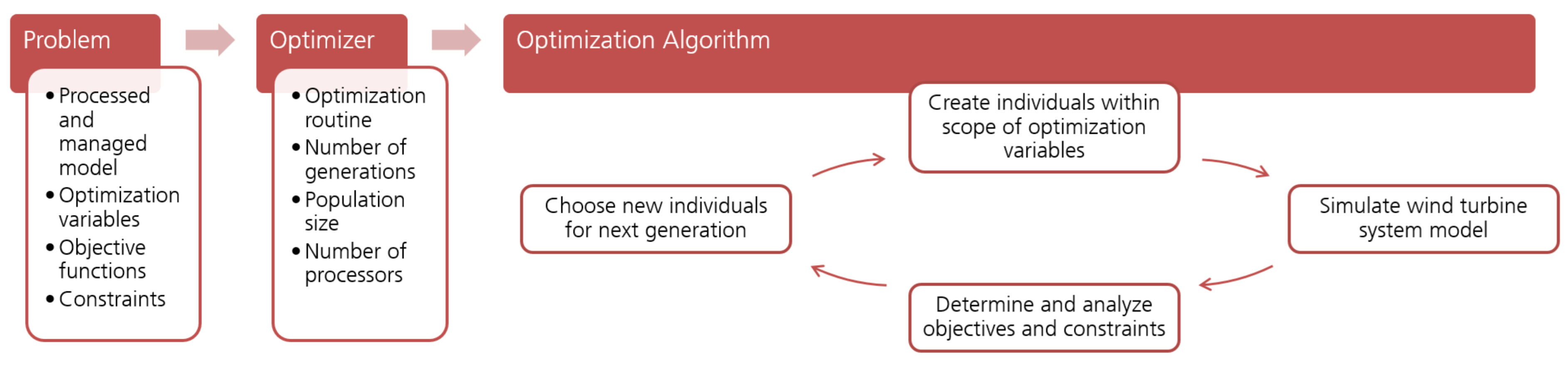
4. Incorporation of Optimization Functionalities

By incorporating additional functionalities and features, the framework for automated simulation can be extended to be also used for simulation-based optimization, as defined by Gosavi [56]. Such an automated optimization procedure is highly beneficial because wind turbine systems cannot directly be optimized just by utilizing mathematical operations, as the non-linear system is too complex (with even much greater complexity in case of floating wind turbine systems), and, thus, optimization tasks on wind turbine systems come with several iterations—corresponding to a large number of simulations—until the optimum solution is found.
The programming framework, as introduced in Section 2.3, serves as basis. The extension happens mainly in the step for defining the execution of the task (Section 2.3.3), as visualized in Figure 2. At this point, the optimization task has to be introduced, specified through the optimization problem (Section 4.1), the optimizer (Section 4.2), and the optimization algorithm (Section 4.3), as explained in detail in the following and presented schematically in Figure 3.

4.1. The Optimization Problem

First, the optimization problem (left part in Figure 3) has to be defined to specify the optimization (or so-called design) variables x i , the objectives, and the constraints for both of them. The optimization objectives are expressed in terms of objective functions f i . The constraints could either be equality constraints h i or in-equality constraints g i . Both the objective functions and the (in-)equality constraints can be functions of the design variables, combined in the design variables vector X, as well as further system parameters. Due to the complexity of the fully coupled dynamics of floating wind turbine systems, this dependency on other system parameters is expressed by means of the function s y s t e m ( X ) . Thus, such an optimization problem can be generally formulated as follows:
find X = x 1 , . . . , x k to minimize f i ( X , s y s t e m ( X ) ) , i = 1 , . . . , l subject to h i ( X , s y s t e m ( X ) ) = 0 , i = 1 , . . . , m subject to g i ( X , s y s t e m ( X ) ) 0 , i = 1 , . . . , n

4.1.1. Optimization Variables

Within an optimization task there are parameters of the wind turbine system selected, which may be modified during the optimization. These optimization variables are specified, using the parameter names according to the model definition.

4.1.2. Objective Functions

Apart from the modifiable wind turbine system parameters, the specific goal of the optimization has to be specified, but also several objectives can be pursued within one optimization task. These goals are defined through objective functions—expressions which are to be (depending on the specific optimization routine, but typically) minimized. Using a parameter ( c r i t e r i o n ), taken from simulation results or from further processing of these, and having the target value ( g o a l ) for this criterion, possible notations of the objective function could be for example Equations (1) and (2), with or without using a normalization, respectively. If no target value is prescribed and the parameter directly is to be minimized (or maximized), just c r i t e r i o n (or c r i t e r i o n ) is given as expression.
c r i t e r i o n g o a l g o a l
c r i t e r i o n g o a l
Such expressions can be set up for each objective; however, in that case, the optimizer has to be capable of processing multiple objective functions at the same time. In the other case, if the used optimizer is not a multi-objective (MO) one and, thus, can only cope with one single objective function, all goals have to be written in one equation. In this case, typically weight factors ( w e i g h t ) are incorporated, which allow for differentiating the importance of the single objectives. Thus, the objective function for N goals could be written for example as in Equations (3) and (4), considering the same two cases with or without normalization of the objective.
i = 1 N w e i g h t i c r i t e r i o n i g o a l i g o a l i
i = 1 N w e i g h t i c r i t e r i o n i g o a l i

4.1.3. Constraints

The optimization variables, goals, and also other system parameters may be constrained, meaning that only specific values are allowed for these parameters to take on or certain dependencies or relations between parameters exist.
The values, which the design variables may take on, are commonly constrained. Thus, the allowable value ranges, provided in terms of lower and upper limits, have to be declared for each of the optimization variable.
In addition to the specified objective functions, the goals might also be constrained or have to stand in a defined relation to each other. In such a case of having a constrained problem, additional equations for the limiting conditions are to be provided. When, for example, using the objective function given in either Equations (1) or (2), which is to be minimized, but also wanting to constrain the criterion to approach the goal from the left side on the numerical scale, meaning not exceeding the target value, the constraint can be defined as given in Equation (5).
c r i t e r i o n g o a l 0
In optimization scripts, which separate the parameter relation (left-hand side of Equation (5)) from the (in-)equality constraint (≤#, ≥#, =#, ≠#, with a number #), the code might be simplified if all constraint equations are converted into such a formulation, that all use the same (in-)equality constraint. Then, the left-hand side expressions can be provided as vector input, while for the (in-)equality constraint only one type needs to be specified.

4.2. The Optimizer

Having the optimization problem defined, an optimizer has to be selected for executing the optimization algorithm and, thus, solving the optimization task. A variety of available optimizers is presented in Table 1. The optimizers are grouped according to their basic method into Quasi-Newton method, Sequential Quadratic Programming (SQP), Evolutionary Algorithm (EA), Particle Swarm Optimization (PSO), and other types. Furthermore, it is indicated if the optimization routine requires gradients or if it is a gradient-free method. Another important feature is the capableness of the optimizer to handle multi-objective problems, which is already mentioned in Section 4.1. Thus, in Table 1 it is additionally indicated which optimizers can process multiple objective functions.
Due to the iterative character of optimization routines, there is the need to specify a stop criterion to limit the number of iterations and terminate the optimization algorithm at a specific point. Most commonly, two options for setting such a stop criterion exist: defining a convergence tolerance for terminating the optimization routine or setting an upper limit to the number of iterations performed.
Some more additional parameters have to be defined when using optimizers which fall in the category of EAs. These basically work according to the same principle as Darwin’s theory of evolution. One advantage of EAs is that they are gradient-free methods, which might be highly relevant when dealing with complex systems, such as an aero-hydro-servo-elastic wind turbine, where the system complexity can no longer be minimized and represented by means of one single system equation. Thus, EAs might be very suitable for finding the global optimum for even multi-objective optimization problems for highly complex engineering systems [60]. The main inputs, required for EA-based optimization routines, are presented in the following:
  • Population size:
    As EAs work with populations, in which the individuals are modified from generation to generation, the number of individuals in each generation, meaning the size of the population, has to be provided. According to this number, a randomly distributed start population (generation 0) is created within the prescribed value ranges of the design variables. Depending on the fitness of each individual—meaning how good the individual is in terms of the objectives—as well as its compliance with the specified constraints, some individuals are selected, or recombined, or mutated, and a new set of individuals is created as population of the next generation.
  • Number of generations:
    The iterative generation of populations continues until a stop criterion is reached. This is mostly a maximum number of generations to be created and simulated. Thus, the number of generations has to be specified and given as input to the optimizer.
  • Number of processors:
    With the ability of running simulations in parallel—depending on the capabilities of the programming framework and computer system—the number of processors can be provided as well. This option of multi-processing is highly beneficial for optimization applications, as it allows for parallel simulation of several individuals of one generation.
The inputs to the optimizer are presented in the second step in Figure 3 on the example of an EA-based optimization routine.

4.3. The Optimization Algorithm

The final step is the execution of the iterative optimization algorithm, following the specified optimization problem (Section 4.1) and using the defined optimizer (Section 4.2). According to the optimization routine and prescribed value ranges, values for the design variables are set and the wind turbine system model is simulated. If this was successful, the simulation results are analyzed internally by the optimizer, based on the prescribed objective functions and constraints. If, however, the simulation failed—due to bad system performance—and, thus, the specified simulation duration is not completed, the criterion for evaluating the objective function might not be existing or used. For such a case a different approach, handling such unsuccessful simulations, can be coded within the optimization algorithm. This might be, for instance, to directly set the goals to suboptimal values and therefore step over the evaluation of the objective functions or to include additional constraints, by which means the initial system integrity, conformity, or stability—for example, for a floating offshore wind turbine—is checked. Based on these analyses of objectives and constraints, new values within the prescribed boundaries are selected by the optimizer and assigned to the design variables. Then, the algorithm is repeated until the stop criterion is reached.
The optimization algorithm is presented in the right part in Figure 3 on the example of an EA-based optimization routine. In this case, several simulations are executed within each iteration, so that p o p u l a t i o n s i z e n u m b e r o f g e n e r a t i o n s simulations are run during the entire optimization procedure. The optimization procedure starts with generating the first individuals according to the set value ranges of the optimization variables. Afterwards, each individual wind turbine system model is simulated, the criteria are extracted from the simulation results, and the objective functions, as well as the constraints, are evaluated. Based on these analyses, a new set of individuals for the next generation is chosen by the optimizer, again complying with the allowable value ranges of the design variables. At this point, the optimization procedure is repeated until the specified maximum number of generations and, hence, the stop criterion, is achieved.
To save the results of each simulated wind turbine system model, which is created during the optimization algorithm, the already coded commands when processing the model in the programming framework (as mentioned in Section 2.3.1) might be supplemented by additional code. This way, for example, also the evaluated objectives of each simulation can be written in addition to the output parameters in an output file and used later on for further post-processing or visualization of the progression of the objective functions and design variables.

5. Application of the Framework to Optimization Tasks for Wind Turbine Systems

In the following, three different examples, realized with the exemplary programming framework described in Section 2.3.5, are presented to show the functionality, technical feasibility, and the broad application range of the presented framework for automated simulation and optimization. The optimizers are taken from open-source frameworks, such as OpenMDAO (http://openmdao.org/twodocs/versions/latest/tags/Optimizer.html#optimizer, accessed on 12 October 2018) (Multi-disciplinary Design, Analysis, and Optimization) or Platypus (https://platypus.readthedocs.io/en/latest/, accessed on 12 October 2018), which are both programmed in Python.

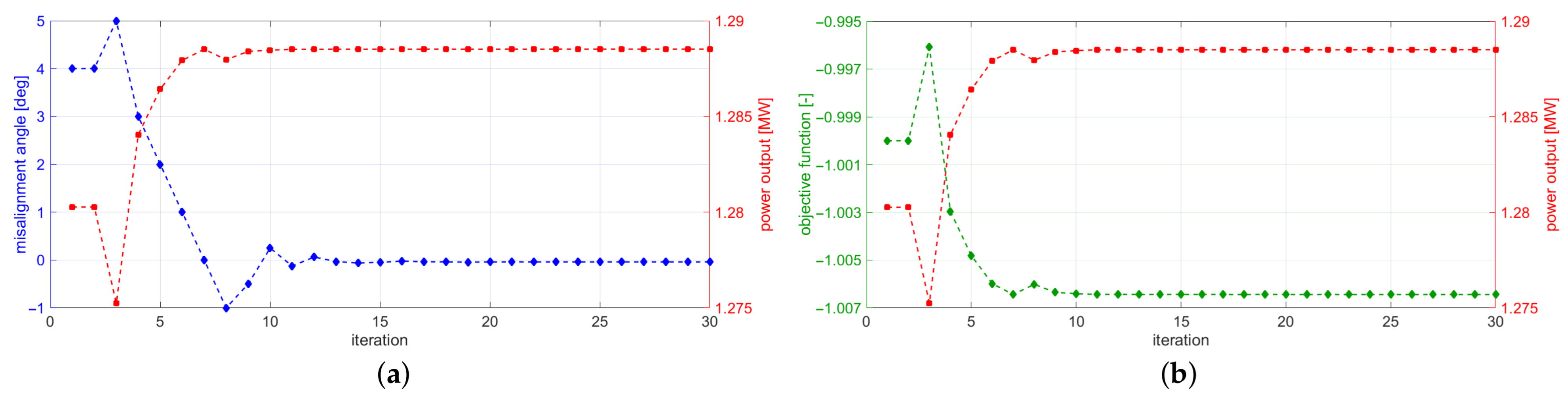
5.1. Plausibility Check of an Optimization Routine

Since optimization problems and wind turbine systems are very complex, it is difficult to assess the results from an optimization procedure. Thus, first, a test case is implemented in the MoWiT-Dymola®-Python framework to check the proper functioning of the established framework, as well as the plausibility of the optimization routine. The NREL 5 MW reference wind turbine [61] is used, operating at a constant wind speed of 7 m/s, which is below rated wind speed. Now, any control system—apart from the generator control—is turned off, so that neither the blades are pitched nor the rotor-nacelle-assembly is yawed for controlling optimum operation. Having the control systems disabled, an initial misalignment between the wind direction and the normal of the rotor plane is initiated. The optimization problem is then to change the value of the misalignment angle in order to achieve maximum power output. From wind physics theory, the maximum power output is expected when the wind direction is perpendicular to the rotor plane (meaning having a zero misalignment angle), as in this case the projected area facing the wind is maximum.
As this optimization problem has a single objective, optimizers from the list presented in Table 1 are selected, which are not MO but gradient-free, as this is required due to the high complexity of the considered wind turbine system. Due to its good performance in preceding comparative simulations with various gradient-free and single-objective optimizers, the presented optimization problem is realized with the optimizer COBYLA from OpenMDAO [57]. Here, it has to be noted that the framework does not rely on this specific optimizer, which is just selected due to its computational efficiency for the presented optimization problem to verify the correct functioning of the developed simulation and optimization framework. For defining the objective function, the mean power output p o w e r i is taken for each iteration i from the simulation time series, excluding the transients at the beginning. The objective function, which is to be minimized, is then determined following Equation (6).
f = p o w e r i p o w e r 1
The initial misalignment angle is exemplarily set equal to 4°—another value would only affect slightly the convergence rate. The results of the optimization procedure, which are obtained after half an hour of successive simulations, are shown in Figure 4, presenting the progression of the optimization variable in terms of the misalignment angle (Figure 4a), as well as the trend of the objective function (Figure 4b), both together with the resulting power output—the optimization goal. 30 iterations are performed and presented; however, it can be seen that a steady state is already reached after around 15 iterations. Furthermore, the results match the expectations and, thus, the functionality of the optimization routine, incorporated in the framework, is approved.

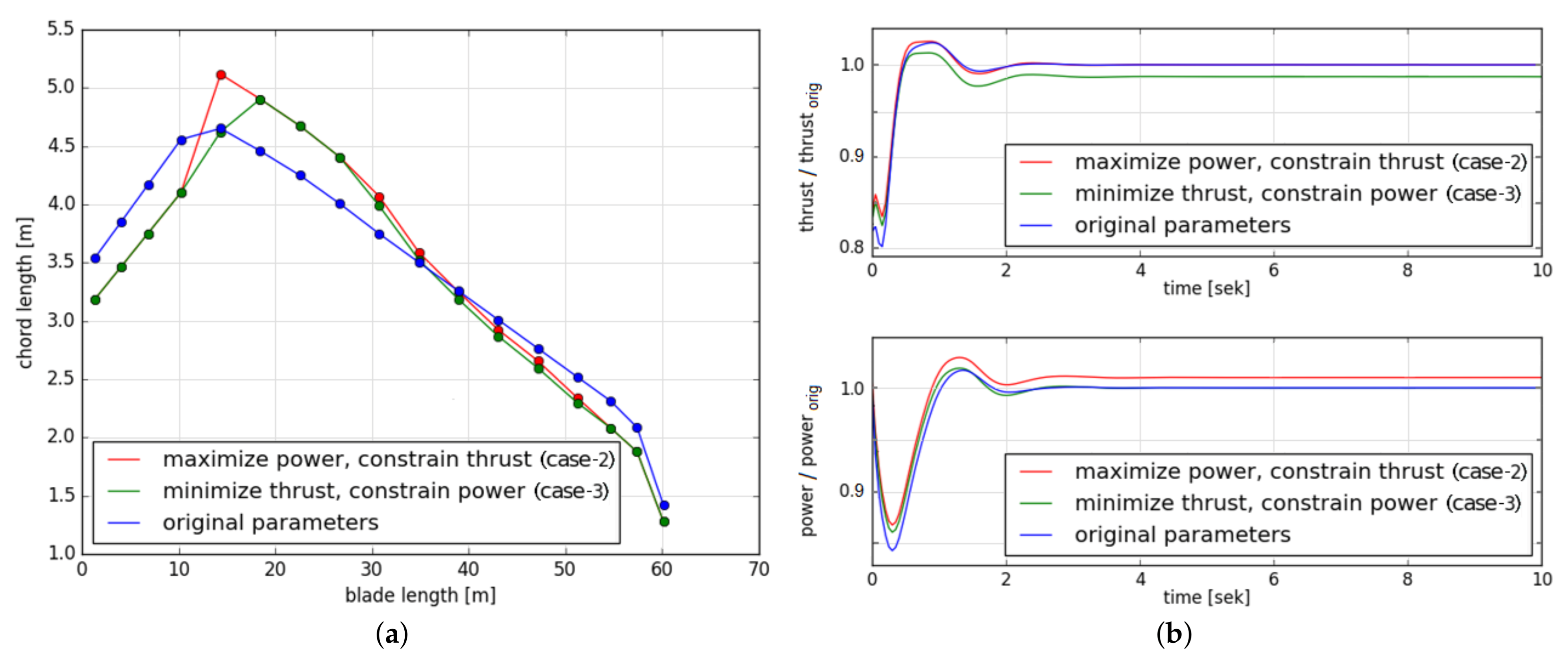
5.2. Power Output vs. Thrust Force

Within the wind industry, yield increase—governed by the power output of a wind turbine—is a common goal; however, one should not forget about the loads on the wind turbine, represented for example by the thrust force on the rotor. These two parameters show contradictory demands: Maximum exploitation of the wind resource and, hence, increasing the power output for one and the same wind speed leads to an increase in the rotor thrust as well, and vice versa. Both parameters are influenced by the shape of the rotor blades. Thus, in this optimization problem, the NREL 5 MW reference wind turbine [61] is used again, operating at a constant wind speed and having each blade defined through 17 sections. The optimization variable is now the chord length, which independently can be modified at each of the 17 sections along the rotor blade. If doing this professionally, also other blade parameters would have to be adjusted and the simulations would have to be performed at different wind speeds and evaluated according to the wind speed distribution prevailing at the considered site; however, in this example, the optimization problem is kept simple, as it should mainly deal as a demonstration case for optimization with two contrary objectives.
For this optimization problem (case-1), basically, two objectives are then to be defined: the maximization of the rotor power output and the minimization of the rotor thrust force. The combination of both objectives into one objective function is realized by utilizing weight factors ( w e i g h t p o w e r and w e i g h t t h r u s t ) for power and thrust, respectively, as presented in Equation (7).
f case 1 = w e i g h t t h r u s t t h r u s t i t h r u s t 1 w e i g h t p o w e r p o w e r i p o w e r 1
Optimization simulations are performed with different gradient-free (due to the same reason of the highly complex wind turbine system, as already stated in Section 5.1) and single-objective optimizers from OpenMDAO, such as COBYLA and ALPSO [57], in order to test the capability of single-objective optimizers being applied to MO optimization problems. The opposing goals challenge the optimizers and show the limited use of single-objective optimizers, which still can work with several goals, which, however, have to be written in one objective function. The final “optimum” solution highly depends on the user-defined and, thus, quite arbitrary chosen weight factors for the objectives and, therefore, cannot represent one real unbiased optimum.
The influence of the weight factors can be demonstrated when considering the two boundary events: Only one of the objectives is relevant, the other one is neglected—or, more explicitly, just used as constraint. Thus, still using the OpenMDAO optimizers, the optimization problem is modified and adjusted so that in one task (case-2) the power output is to be maximized and the thrust force is limited by not exceeding the original value t h r u s t orig (as represented by Equation (8)), while in the other task (case-3) the thrust force minimization is defined as objective and the power output is constrained by not falling below the original value p o w e r orig (as written in Equation (9)).
f case 2 = p o w e r i p o w e r 1 and t h r u s t i t h r u s t orig
f case 3 = t h r u s t i t h r u s t 1 and p o w e r i p o w e r orig
For each of the two optimization tasks (case-2 and case-3), an optimum is obtained after around two hours of successive simulations; however, with this approach also two different optimum blade shapes are achieved, as visualized in Figure 5a, for which each is only the best for each case, as shown in Figure 5b. Thus, this again emphasizes the relevance of utilizing more holistic and multidisciplinary approaches and using optimizers that are capable of handling multiple objectives at the same time.

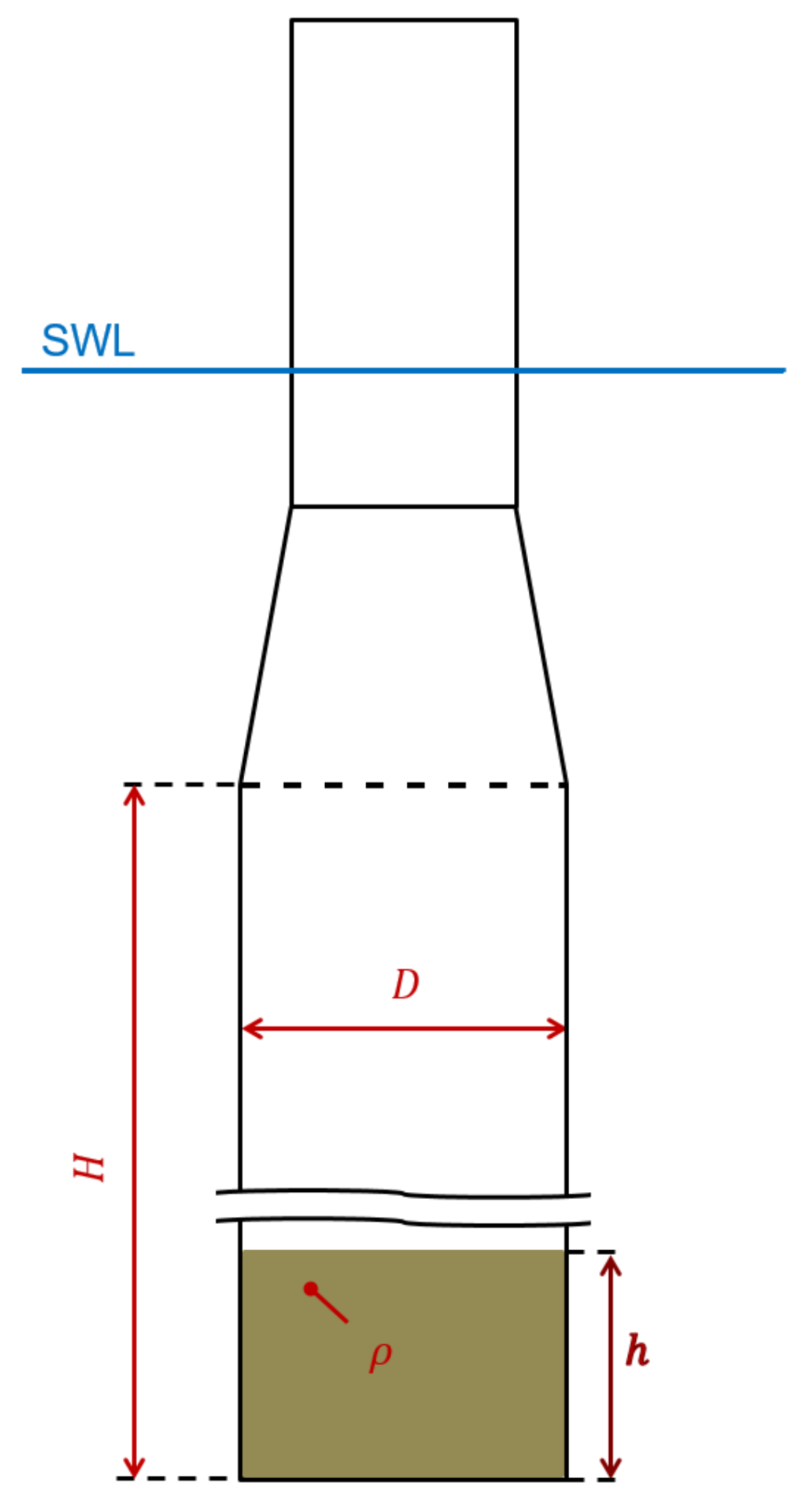
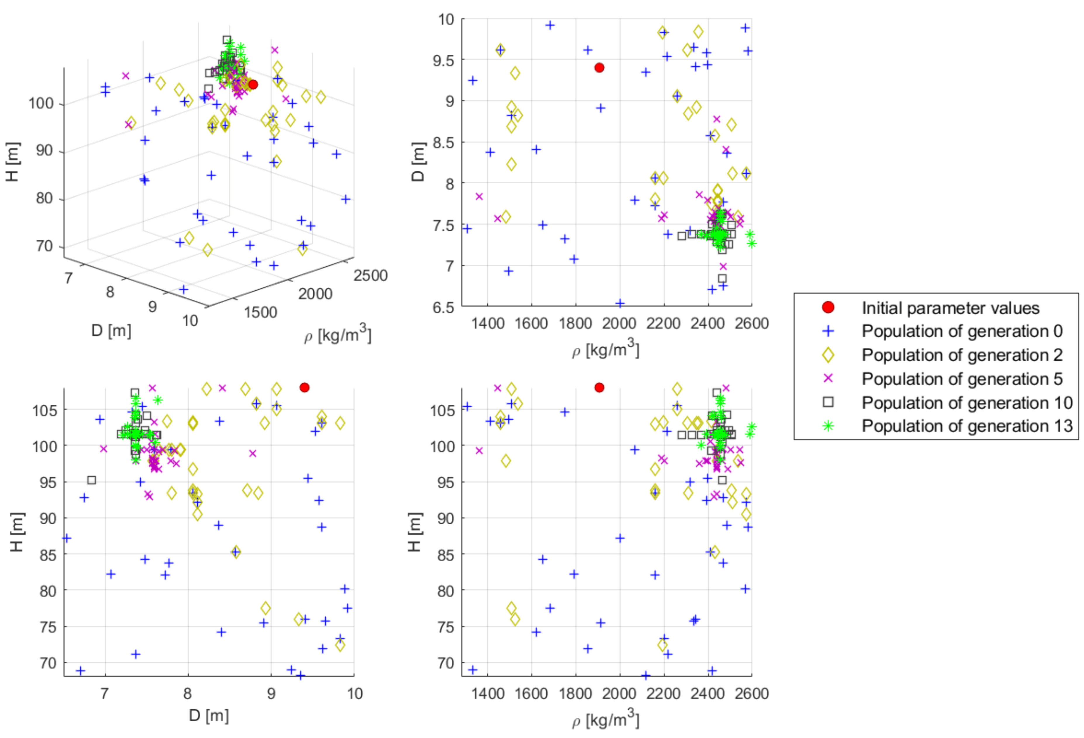
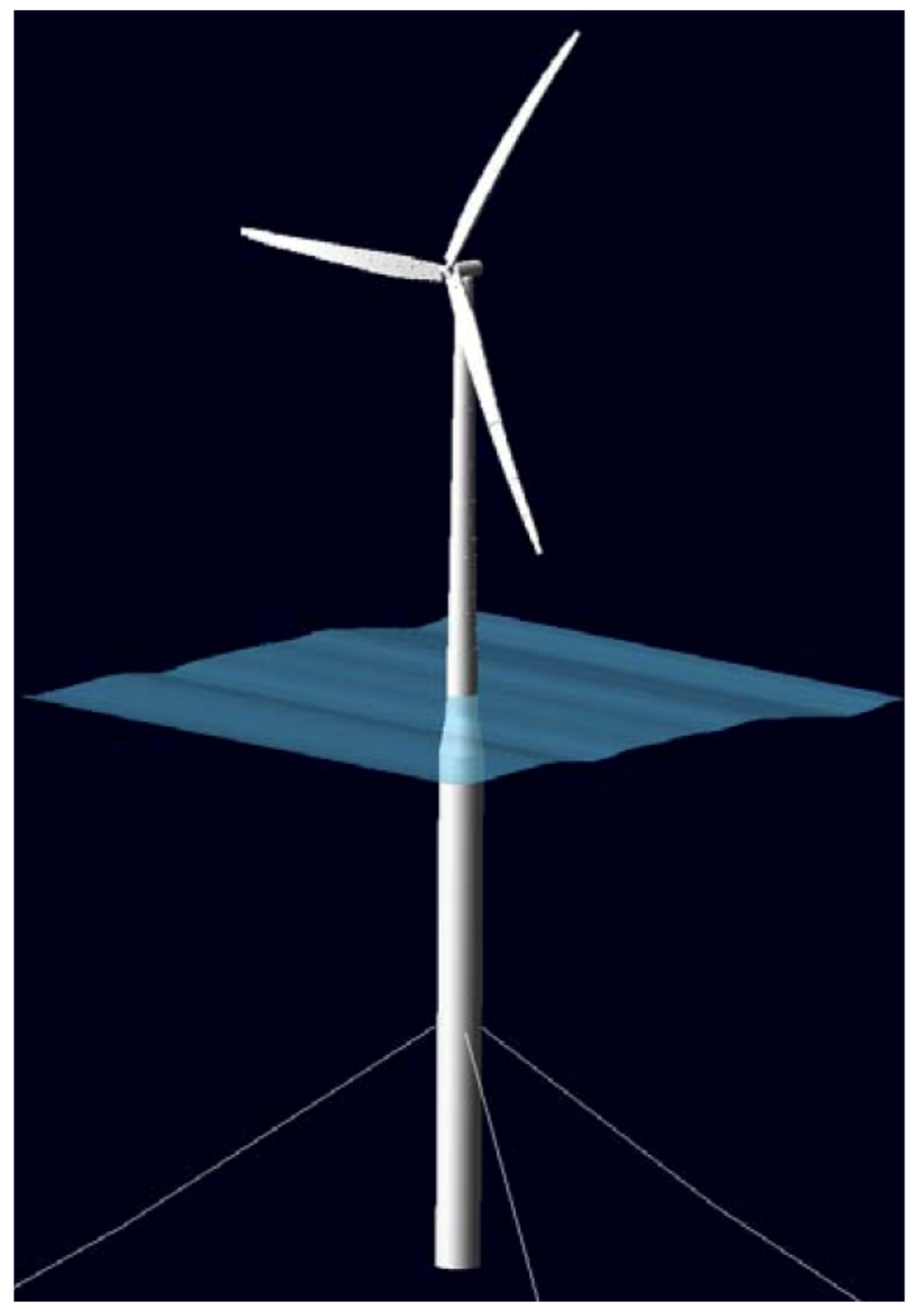
5.3. Floater Design Optimization

Developing wind turbine systems requires several iterations, revisions, and optimization steps. Design drivers in the wind industry are among others costs—both capital and operational expenditure—and, thus, in total the levelized cost of energy. Especially for the emerging sector of floating wind energy, economic efficiency is very important to achieve competitiveness with conventional and other renewable energy sources. Thus, design optimization of floating wind turbine systems is a relevant topic.
This optimization task can be approached in different ways. Mostly, optimization variables in a design process are geometric parameters. Thus, shape, dimensions, and structural properties of the floating platform might be modified, while the supported wind turbine remains in most respects—and apart from, for example, controller tuning as pointed out in Section 6—unchanged. Based on survey results by Leimeister et al. [62], relevant objective criteria are, besides the levelized cost of energy, also maintenance aspects (including the reliability of the components), the potential of serial production (meaning, for example, modular structures), and the system performance. The latter criterion implies certain requirements and limits for the system response, such as nacelle acceleration, platform inclination, or translational motion, which are prescribed by specifications of single wind turbine components.
Thus, the developed MoWiT-Dymola®-Python framework is applied to a design optimization task, which is shortly introduced as well in [31] and intensified in [42], using the NREL 5 MW reference wind turbine [61] on top of a floating spar-buoy, as described in OC3 (Offshore Code Comparison Collaboration) phase IV [63] and shown in Figure 6. In this example, three parameters of the floating platform are selected as design variables, as displayed in Figure 7:
  • The diameter D of the spar-buoy column;
  • The height H of the spar-buoy column;
  • The density ρ of the ballast.
To maintain the system hydrostatic stability, the ballast height h is finally internally adjusted depending on the values of these three design variables.
As already mentioned at the beginning of this section, the design is cost-driven; however, it is also well known that—especially in case of innovative technologies and concepts—unnecessarily high safety factors are applied, which in return make the design more costly again. This can be as well observed in case of the OC3 floating spar-buoy wind turbine system, which is heavily over-dimensioned. To address this issue—keeping in mind the overall goal of limiting the system costs—the optimization task refers to reducing the unnecessarily high safety factors, meaning to design a floating wind turbine system which is still safely operating but close to the operational limits, while constraining the outer floater dimensions what itself entails a potential cost reduction. Thus, the diameter and height of the spar-buoy column are constrained, as presented in Table 2, while the optimization itself focuses on the global system performance, using the maximum values of system inclination, nacelle acceleration, and floater translation for defining the objective functions. For inclination and acceleration it is aimed to reach a certain target value, which corresponds to the maximum allowable value for a wind turbine system during operation [64,65,66,67,68], while the translational motion is to be minimized in general. The specific constraints of the optimization problem are presented in Table 2.
In order to extract the system performance criteria, the floating wind turbine has to be evaluated in operating conditions. To reduce the computational effort, simulations with the original OC3 spar-buoy floating system are performed for the preselected DLCs 1.1, 1.3, and 1.6, according to IEC 61400-3-1 [1] and utilizing the developed framework for automated execution of simulations. For the simulated environmental conditions, extreme responses of the floating system with respect to system inclination and translational motion, as well as the nacelle acceleration, are expected [42]. From the time series, the DLCs with the highest values for the specified objectives are extracted and DLC 1.6 at rated wind speed with a yaw misalignment angle of 8° turned out to be the most critical DLC with regard to the optimization objectives. Hence, this environmental condition is used for the floating system simulations within the iterative optimization algorithm. Here, it has to be noted that the framework allows for optimization with integrated automated simulation of several DLCs; however, in this example one critical DLC is selected in advance to be solely used during the optimization—due to limited computational resources—and the obtained optimized design is re-evaluated for the full set of DLCs subsequently.
The optimization is performed with the MO optimizer NSGAII from Platypus, which is an open-source framework focusing especially on MOEAs [58]. This choice is made, as NSGAII:
  • follows a gradient-free method, which is essential for the highly complex floating wind turbine system considered in this optimization task, as already emphasized in Section 5.1 and Section 5.2;
  • is a MO optimizer and, hence, can easily deal with the three distinct objective functions;
  • belongs to the category of EAs, which are highly suitable for finding the global optimum, even when dealing with MO optimization problems and highly complex engineering systems, as already highlighted in Section 4.2;
  • performed in a preceding comparative study, utilizing as well other gradient-free and MO optimizers from Platypus (such as NSGAIII or SPEA2), best with respect to convergence speed and compliance with the constraints.
In each generation, 36 individuals are simulated. The stop criterion is defined through the total number of simulations to be run—set to 900—which indirectly defines the maximum number of generations, corresponding to 25 including the start generation 0. Furthermore, based on the default settings of NSGAII from Platypus, a random generator and a tournament selector, comparing two individuals with each other and selecting the winner based on its dominance, are utilized, while no variator is included. The total compuational time for performing this optimization problem with the fully coupled floating wind turbine system, when utilizing 36 processors for parallel simulation, amounts to 109 h. The development of the individuals through the generations is visualized in Figure 8 and Figure 9 for five selected generations and compared to the initial OC3 floating wind turbine system design. In Figure 8, it can be observed that at the beginning (start generation 0) the entire value ranges of the design variables are used, while during the optimization the spread is decreasing to an already quite narrow selection area in generation 13, which refers to different parameters compared to the original OC3 spar-buoy design. With increasing number of simulated generations, the spread in the specified objectives decreases as well and the objectives themselves improve more and more, meaning that they take on smaller and smaller values, as shown in Figure 9. For the final selection of one optimum solution, various approaches can be followed, but the main point is to show that the individuals obtained through the optimization procedure (e.g., already the individuals in generation 13) are significantly better with respect to the specified criteria than the initial OC3 floater design, which can clearly be seen in Figure 9, while the outer dimensions of the floating spar-buoy can be reduced, as apparent from Figure 8, which implies material and, thus, cost savings.

6. Future Developments

Apart from the three examples, outlined in Section 5, the presented framework has a broad range of applications to various optimization tasks for wind turbine systems:
  • As already presented in Section 5.3, design optimization is a key application, useful and required within the design process of a wind turbine system (either the whole system or only single components, such as the tower, support structure, or even the mooring system in case of a floating offshore wind turbine). The focus of interest within such a design optimization could range from costs and material usage, loads and lifetime, as well as system performance and response, as pointed out in Section 1. The presented framework tool can, thus, be used, for example, just for obtaining a fast preliminary design to do a cost estimation for the initial planning of ((floating) offshore) wind turbines or—on the other hand—for a very detailed reliability-based design optimization to improve the system reliability and, this way, reduce the downtime of an offshore (floating) system due to defects and long waiting times for proper weather windows for doing maintenance and repair work.
  • Apart from the more structural-based design optimization, also the control system of the wind turbine needs to be tuned and optimized for the specific purpose. The control system is an essential component, which regulates the wind turbine performance. By pitching the blades, the amount of power extracted from the wind, as well as the thrust force acting on the rotor, are influenced. Below rated wind speed, the blades are not pitched so that the maximum possible power can be extracted, while above rated wind speed, the blade pitch angle is regulated to maintain constant power output or generator torque (depending on the wind turbine control method), which at the same time reduces the thrust force on the rotor. Two main parameters are the proportional and integral gains of the PI controller. Thus, with tuning the controller parameters, different optimization goals can be pursued:
    -
    Controller optimization for load reduction:
    The goal is to reduce oscillations in the sensor generator speed and to achieve as early as possible a steady state. This implies at the same time also reduced oscillations and an earlier steady state in the power output, blade pitch angle, and the loads on the turbine.
    -
    Controller adaption for floating systems:
    Wind turbine controllers measure the wind speed in certain intervals. In case of a floating system, the measured speed is not undisturbed but the resulting wind speed due to wind inflow and motion of the floating system. A common onshore or bottom-fixed offshore wind turbine controller is much faster than the floating platform motions. This means that the time intervals for taking measurements are so small, that the controller would perceive a decreasing wind speed (corresponding to a decreasing rotor thrust) if the floating system moves with the wind. The reaction of the controller would then be to pitch the blades into the wind to avoid a reduction of the power output. This, however, will increase the thrust force and the system will continue moving backwards. This negative damping effect, which would be introduced when using a common onshore-type wind turbine controller for a floating offshore system, therefore leads to an unstable system behavior. For this reason, the controller parameters would have to be adjusted. Thus, the optimization goal in this case is to tune the controller in order to obtain a stable floating system, with a controller frequency lower than the smallest eigenfrequency of the floating wind turbine system. This tuning can be done through running iterative simulations within an optimization algorithm [69].
  • Considering an entire wind farm, the framework tool can also be applied to optimize the wind farm layout with regard to the space utilized and power extracted, as already outlined in Section 1. Another option for maximizing the power output of the entire wind farm—having a fixed layout—is to adjust the control and operational management of the single wind turbines by, for instance, changing the yaw angle of the first rows’ turbines to influence the wake direction and the flow condition reaching the turbines behind.
In addition to the high flexibility in the application to optimization tasks, the framework is not only suitable for optimization problems, but also directly for executing automatically a large number of simulations, which is, for example, required in DLC analyses. Both capabilities of the framework can be utilized at the same time by incorporating a set of DLC simulations within the execution of the optimization algorithm. Furthermore, if using another library as basis, the framework is not limited to wind turbine systems and can be applied to other complex engineering systems as well.
However, in any application of the framework for automated simulation and optimization, especially when using it for optimization tasks, the specific settings have to be chosen carefully—including a sensitivity study where appropriate. Thus, for instance, the results and success of the optimization highly depend on the optimization settings and employed optimizer. The example in Section 5.1 approved the proper and fast functioning of the single-objective optimizer COBYLA, while the optimization task in Section 5.2 showed its limited suitability for two (or more) contrary objectives. On the other hand, a MO optimizer, such as NSGAII, proved to be capable of easily handling complex problems with several design variables, objectives, and constraints, as presented in Section 5.3.

7. Conclusions

This paper presents the development of a holistic and highly flexible framework for automated simulation and optimization of wind turbine systems, including all system components and their fully coupled aero-hydro-servo-elastic behavior. Compared to other existing optimization approaches, which are mostly tailored to one or a few specific optimization tasks and a very limited number of components of interest, the developed framework is based on a fully modular, automated, and high-fidelity approach, which uses systematic methods, does not need any approximations, and is very flexible and adaptable. Thus, this framework can be used for automated execution and analysis of DLC simulations, as well as for running optimization algorithms, in which the automated simulation execution can still be employed. The framework requires a modeling environment, a simulation engine, as well as the programming framework itself. In case of optimization tasks, the optimization problem, optimizer, and optimization algorithm have to be defined as well. The broad range of applications of such an optimization framework for wind turbine design is shown on the example of the MoWiT-Dymola®-Python framework, with the highly flexible modeling environment MoWiT, coupled to the simulation engine Dymola®, and the extremely advantageous programming language Python. The technical feasibility and proper functioning of this framework is first verified by means of a plausibility check. Suitable application cases are, for instance, the optimization of the wind turbine performance (power output) and loading (thrust force), the design optimization of, for example, the support structure of a floating wind turbine, the tuning of the wind turbine controller for load reduction or adjustment to different (floating) wind turbine systems, or different optimization tasks within wind farms. All in all, such a framework has high relevance in design and analysis processes of wind turbine systems, as these come with a large number of (iterative) simulations. Thus, the presented framework for automated simulation and optimization forms the basis for sophisticated industrial applications and advanced design optimization tasks, including reliability aspects as well, in the field of floating offshore wind.

Author Contributions

Conceptualization, M.L.; methodology, M.L.; software, M.L.; validation, M.L.; formal analysis, M.L.; investigation, M.L.; data curation, M.L.; writing—original draft preparation, M.L.; writing—review and editing, M.L., A.K. and M.C.; visualization, M.L.; supervision, A.K. and M.C.; project administration, M.L.; funding acquisition, A.K. All authors have read and agreed to the published version of the manuscript.

Funding

This work was partially supported by grant EP/L016303/1 for Cranfield University, University of Oxford and University of Strathclyde, Centre for Doctoral Training in Renewable Energy Marine Structures—REMS (http://www.rems-cdt.ac.uk/) from the UK Engineering and Physical Sciences Research Council (EPSRC) and the German Fraunhofer Institute for Wind Energy Systems (Fraunhofer IWES).

Institutional Review Board Statement

Not applicable.

Informed Consent Statement

Not applicable.

Data Availability Statement

Not applicable.

Acknowledgments

The authors want to thank Julia Eis for her contribution during her time as student assistant at Fraunhofer IWES and Philipp Thomas for his supervision at Fraunhofer IWES.

Conflicts of Interest

The authors declare no conflict of interest.

Abbreviations

The following abbreviations are used in this manuscript:
ALPSOAugmented Lagrangian PSO
BFGSBroyden-Fletcher-Goldfarb-Shanno
CMAESCovariance Matrix Adaptation Evolution Strategy
COBYLAConstrained Optimization BY Linear Approximation
CONMINCONstrained function Minimization
DLCDesign Load Case
Dymola®Dynamic modeling laboratory
EAEvolutionary Algorithm
EpsMOEASteady-state Epsilon-MOEA
FASTFatigue, Aerodynamics, Structures, and Turbulence
FSQPFeasible SQP
GAGenetic Algorithm
GDE3Generalized Differential Evolution 3
HAWC2Horizontal Axis Wind turbine simulation Code 2nd generation
IBEAIndicator-Based EA
IECInternational Electrotechnical Commission
IPOPTInterior Point OPTimizer
IWESInstitute for Wind Energy Systems
L-BFGS-BLimited-memory BFGS with Box constraints
MOMulti-Objective
MOEADMO EA based on Decomposition
MoWiTModelica® library for Wind Turbines
Newton-CGNewton Conjugate Gradient
NOMADNon-linear Optimization by Mesh Adaptive Direct search
NRELNational Renewable Energy Laboratory
NSGAIINon-dominated Sorting GA II
NSGAIIINon-dominated Sorting GA III
OC3Offshore Code Comparison Collaboration
OMOPSOOur multi-objective PSO
OpenMDAOOpen-source Multi-disciplinary Design, Analysis, and Optimization
PEASParallel EAs
PESA2Pareto Envelope-based Selection Algorithm
PSOParticle Swarm Optimization
PSQPPreconditioned SQP
SLSQPSequential Least Squares Quadratic Programming
SMPSOSpeed-constrained multi-objective PSO
SNOPTSparse Nonlinear OPTimizer
SPEA2Strength Pareto EA 2
SQPSequential Quadratic Programming
TNCTruncated Newton

References

  1. International Electrotechnical Commission. Wind Energy Generation Systems—Part 3-2: Design Requirements for Floating Offshore Wind Turbines: Technical Specification IEC TS 61400-3-2; International Electrotechnical Commission: Geneva, Switzerland, 2019. [Google Scholar]
  2. International Electrotechnical Commission. Wind Energy Generation Systems—Part 3-1: Design Requirements for Fixed Offshore Wind Turbines: International Standard IEC 61400-3-1; International Electrotechnical Commission: Geneva, Switzerland, 2019. [Google Scholar]
  3. DNV GL AS. Loads and Site Conditions for Wind Turbines: Standard DNVGL-ST-0437; DNV GL AS: Oslo, Norway, 2016. [Google Scholar]
  4. Baños, R.; Manzano-Agugliaro, F.; Montoya, F.G.; Gil, C.; Alcayde, A.; Gómez, J. Optimization methods applied to renewable and sustainable energy: A review. Renew. Sust. Energ Rev. 2011, 15, 1753–1766. [Google Scholar] [CrossRef]
  5. Momoh, J.A.; Surender Reddy, S. Review of optimization techniques for Renewable Energy Resources. In Proceedings of the PEMWA 2014, Milwaukee, WI, USA, 24–26 July 2014; pp. 1–8. [Google Scholar] [CrossRef]
  6. Härer, A. Optimierung von Windenergieanlagen-Komponenten in Mehrkörpersimulationen zur Kosten- und Lastreduktion. Master’s Thesis, Stiftungslehrstuhl Windenergie Universität, Stuttgart, Germany, 2013. [Google Scholar]
  7. Mytilinou, V.; Kolios, A.J. A multi-objective optimisation approach applied to offshore wind farm location selection. J. Ocean Eng. Mar. Energy 2017, 3, 265–284. [Google Scholar] [CrossRef] [Green Version]
  8. Mytilinou, V.; Lozano-Minguez, E.; Kolios, A. A Framework for the Selection of Optimum Offshore Wind Farm Locations for Deployment. Energies 2018, 11, 1855. [Google Scholar] [CrossRef] [Green Version]
  9. Mytilinou, V.; Kolios, A.J. Techno-economic optimisation of offshore wind farms based on life cycle cost analysis on the UK. Renew. Energy 2019, 132, 439–454. [Google Scholar] [CrossRef]
  10. Muskulus, M.; Schafhirt, S. Design Optimization of Wind Turbine Support Structures—A Review. J. Ocean. Wind. Energy 2014, 1, 12–22. [Google Scholar]
  11. Lemmer, F.; Müller, K.; Yu, W.; Schlipf, D.; Cheng, P.W. Optimization of Floating Offshore Wind Turbine Platforms with a Self-Tuning Controller. In Proceedings of the OMAE 2017, Trondheim, Norway, 25–30 June 2017. [Google Scholar] [CrossRef] [Green Version]
  12. Sandner, F.; Schlipf, D.; Matha, D.; Cheng, P.W. Integrated Optimization of Floating Wind Turbine Systems. In Proceedings of the OMAE 2014, San Francisco, CA, USA, 8–13 June 2014. [Google Scholar] [CrossRef] [Green Version]
  13. Wang, L.; Kolios, A.; Luengo, M.M.; Liu, X. Structural optimisation of wind turbine towers based on finite element analysis and genetic algorithm. Wind Energy Sci. Discuss. 2016, 1–26. [Google Scholar] [CrossRef]
  14. Fylling, I.; Berthelsen, P.A. WINDOPT: An Optimization Tool for Floating Support Structures for Deep Water Wind Turbines. In Proceedings of the OMAE 2011, Rotterdam, The Netherlands, 19–24 June 2011; pp. 767–776. [Google Scholar] [CrossRef]
  15. Ashuri, T.; Zaaijer, M.B.; Martins, J.; van Bussel, G.; van Kuik, G. Multidisciplinary design optimization of offshore wind turbines for minimum levelized cost of energy. Renew. Energy 2014, 68, 893–905. [Google Scholar] [CrossRef] [Green Version]
  16. Hou, P.; Zhu, J.; Ma, K.; Yang, G.; Hu, W.; Chen, Z. A review of offshore wind farm layout optimization and electrical system design methods. J. Mod. Power Syst. Clean Energy 2019, 7, 975–986. [Google Scholar] [CrossRef] [Green Version]
  17. Herbert-Acero, J.; Probst, O.; Réthoré, P.E.; Larsen, G.; Castillo-Villar, K. A Review of Methodological Approaches for the Design and Optimization of Wind Farms. Energies 2014, 7, 6930–7016. [Google Scholar] [CrossRef]
  18. Valverde, P.S.; Sarmento, A.J.N.A.; Alves, M. Offshore Wind Farm Layout Optimization - State of the Art. J. Ocean. Wind. Energy 2014, 1, 23–29. [Google Scholar]
  19. Bottasso, C.L.; Bortolotti, P.; Croce, A.; Gualdoni, F. Integrated aero-structural optimization of wind turbines. Multibody Syst. Dyn. 2016, 38, 317–344. [Google Scholar] [CrossRef] [Green Version]
  20. Bottasso, C.L.; Campagnolo, F.; Croce, A. Multi-disciplinary constrained optimization of wind turbines. Multibody Syst. Dyn. 2012, 27, 21–53. [Google Scholar] [CrossRef]
  21. Shen, X.; Chen, J.G.; Zhu, X.C.; Liu, P.Y.; Du, Z.H. Multi-objective optimization of wind turbine blades using lifting surface method. Energy 2015, 90, 1111–1121. [Google Scholar] [CrossRef] [Green Version]
  22. Mo, Q.Y.; Deng, F.; Li, S.S.; Zhang, K.Y. Multidisciplinary Design Optimization for Small Vertical Wind Turbine Design. Appl. Mech. Mater. 2014, 571–572, 1083–1086. [Google Scholar] [CrossRef]
  23. Bortolotti, P.; Sartori, L.; Croce, A.; Bottasso, C.L. Multi-MW wind turbine CoE reduction via a multi- disciplinary design process. In Proceedings of the EWEA 2015, Paris, France, 17–20 November 2015. [Google Scholar]
  24. Deshmukh, A.P.; Allison, J.T. Multidisciplinary dynamic optimization of horizontal axis wind turbine design. Struct. Multidiscip. Optim. 2016, 53, 15–27. [Google Scholar] [CrossRef]
  25. Chew, K.H.; Tai, K.; Ng, E.; Muskulus, M. Analytical gradient-based optimization of offshore wind turbine substructures under fatigue and extreme loads. Mar. Struct. 2016, 47, 23–41. [Google Scholar] [CrossRef] [Green Version]
  26. Pavese, C.; Tibaldi, C.; Zahle, F.; Kim, T. Aeroelastic multidisciplinary design optimization of a swept wind turbine blade. Wind Energy 2017, 20, 1941–1953. [Google Scholar] [CrossRef]
  27. Clauss, G.F.; Birk, L. Hydrodynamic shape optimization of large offshore structures. Appl. Ocean Res. 1996, 18, 157–171. [Google Scholar] [CrossRef]
  28. Bottasso, C.L.; Campagnolo, F.; Croce, A. Multi-disciplinary constrained optimization of wind turbines. In Proceedings of the EWEC 2010, Warsaw, Poland, 20–23 April 2010; pp. 2241–2250. [Google Scholar]
  29. Jureczko, M.; Mężyk, A. Multidisciplinary optimization of wind turbine blades. In Proceedings of the EACWE 2005, Prague, Czech Republic, 11–15 July 2005; pp. 162–163. [Google Scholar]
  30. Lemmer, F.; Müller, K.; Yu, W.; Guzman, R.F.; Kretschmer, M. Qualification of Innovative Floating Substructures for 10 MW Wind Turbines and Water Depths Greater than 50 m: Deliverable D4.3 Optimization Framework and Methodology for Optimized Floater Design. 2016. Available online: https://ec.europa.eu/research/participants/documents/downloadPublic?documentIds=080166e5af3aacba&appId=PPGMS (accessed on 12 February 2021).
  31. Leimeister, M. Python-Modelica Framework for Automated Simulation and Optimization. In Proceedings of the 13th International Modelica Conference, Regensburg, Germany, 4–6 March 2019; Linköping University Electronic Press: Linköping, Sweden, 2019; pp. 51–58. [Google Scholar] [CrossRef] [Green Version]
  32. DNV GL. Bladed User Manual: Version 4.8; DNV GL: Oslo, Norway, 2016. [Google Scholar]
  33. Jonkman, J.; Buhl, M. FAST User’s Guide; Technical Report NREL/EL-500-38230; National Renewable Energy Laboratory: Golden, CO, USA, 2005. [Google Scholar]
  34. Larsen, T.J.; Hansen, A.M. How 2 HAWC2, the User’s Manual; Risø-R-Report Risø-R-1597; Risø National Laboratory: Roskilde, Denmark, 2015. [Google Scholar]
  35. Leimeister, M.; Thomas, P. The OneWind Modelica Library for Floating Offshore Wind Turbine Simulations with Flexible Structures. In Proceedings of the 12th International Modelica Conference, Prague, Czech Republic, 15–17 May 2017; Linköping University Electronic Press: Linköping, Sweden, 2017; pp. 633–642. [Google Scholar] [CrossRef] [Green Version]
  36. Thomas, P.; Gu, X.; Samlaus, R.; Hillmann, C.; Wihlfahrt, U. The OneWind Modelica Library for Wind Turbine Simulation with Flexible Structure—Modal Reduction Method in Modelica. In Proceedings of the 10th International Modelica Conference, Lund, Sweden, 10–12 March 2014; Linköping University Electronic Press: Linköping, Sweden, 2014; pp. 939–948. [Google Scholar] [CrossRef] [Green Version]
  37. Strobel, M.; Vorpahl, F.; Hillmann, C.; Gu, X.; Zuga, A.; Wihlfahrt, U. The OnWind Modelica Library for Offshore Wind Turbines—Implementation and First Results. In Proceedings of the 8th International Modelica Conference, Dresden, Germany, 20–22 March 2011; Linköping University Electronic Press: Linköping, Sweden, 2011; pp. 603–609. [Google Scholar] [CrossRef] [Green Version]
  38. Popko, W.; Robertson, A.; Jonkman, J.; Wendt, F.; Thomas, P.; Müller, K.; Kretschmer, M.; Hagen, T.R.; Galinos, C.; Le Dreff, J.B.; et al. Validation of Numerical Models of the Offshore Wind Turbine From the Alpha Ventus Wind Farm Against Full-Scale Measurements Within OC5 Phase III. J. Offshore Mech. Arct. Eng. 2021, 143, 82. [Google Scholar] [CrossRef]
  39. Robertson, A.N.; Gueydon, S.; Bachynski, E.; Wang, L.; Jonkman, J.; Alarcón, D.; Amet, E.; Beardsell, A.; Bonnet, P.; Boudet, B.; et al. OC6 Phase I: Investigating the underprediction of low-frequency hydrodynamic loads and responses of a floating wind turbine. J. Phys. Conf. Ser. 2020, 1618, 032033. [Google Scholar] [CrossRef]
  40. Leimeister, M.; Kolios, A.; Collu, M. Development and Verification of an Aero-Hydro-Servo-Elastic Coupled Model of Dynamics for FOWT, Based on the MoWiT Library. Energies 2020, 13, 1974. [Google Scholar] [CrossRef]
  41. Popko, W.; Huhn, M.L.; Robertson, A.; Jonkman, J.; Wendt, F.; Müller, K.; Kretschmer, M.; Vorpahl, F.; Hagen, T.R.; Galinos, C.; et al. Verification of a Numerical Model of the Offshore Wind Turbine from the Alpha Ventus Wind Farm within OC5 Phase III. In Proceedings of the OMAE 2018, Madrid, Spain, 17–22 June 2018. [Google Scholar] [CrossRef] [Green Version]
  42. Leimeister, M.; Kolios, A.; Collu, M.; Thomas, P. Design optimization of the OC3 phase IV floating spar-buoy, based on global limit states. Ocean Eng. 2020, 202. [Google Scholar] [CrossRef]
  43. Dassault Systèmes. Dymola: Dynamic Modeling Laboratory: User Manual Volume 1; Dassault Systèmes: Royal Velizy, France, 2015. [Google Scholar]
  44. Dassault Systèmes. Dymola: Dynamic Modeling Laboratory: User Manual Volume 2; Dassault Systèmes: Royal Velizy, France, 2015. [Google Scholar]
  45. McKinney, W. Python for Data Analysis; O’Reilly: Sebastopol, CA, USA, 2013. [Google Scholar]
  46. Jonkman, B.J. TurbSim User’s Guide, Version 1.50; Technical Report NREL/TP-500-46198; National Renewable Energy Laboratory: Golden, CO, USA, 2009. [Google Scholar]
  47. International Electrotechnical Commission. Wind Turbines—Part 1: Design Requirements; International standard IEC 61400-1; International Electrotechnical Commission: Geneva, Switzerland, 2005. [Google Scholar]
  48. DNV GL AS. Floating Wind Turbine Structures: Standard DNVGL-ST-0119; DNV GL AS: Oslo, Norway, 2018. [Google Scholar]
  49. Det Norske Veritas AS. Design of Offshore Wind Turbine Structures: Offshore Standard DNV-OS-J101; DNV GL AS: Oslo, Norway, 2014. [Google Scholar]
  50. Stieng, L.E.S.; Muskulus, M. Load case reduction for offshore wind turbine support structure fatigue assessment by importance sampling with two–stage filtering. Wind Energy 2019, 22, 1472–1486. [Google Scholar] [CrossRef] [Green Version]
  51. Krieger, A.; Ramachandran, G.K.V.; Vita, L.; Alonso, P.G.; Almería, G.G.; Berque, J.; Aguirre, G. Qualification of Innovative Floating Substructures for 10 MW Wind Turbines and Water Depths Greater than 50 m: Deliverable D7.2 Design Basis. 2015. Available online: http://lifes50plus.eu/wp-content/uploads/2015/11/D72_Design_Basis_Retyped-v1.1.pdf (accessed on 12 February 2021).
  52. Matha, D.; Sandner, F.; Schlipf, D. Efficient critical design load case identification for floating offshore wind turbines with a reduced nonlinear model. J. Phys. Conf. Ser. 2014, 555. [Google Scholar] [CrossRef] [Green Version]
  53. Bachynski, E.E.; Etemaddar, M.; Kvittem, M.I.; Luan, C.; Moan, T. Dynamic Analysis of Floating Wind Turbines During Pitch Actuator Fault, Grid Loss, and Shutdown. Energy Proc. 2013, 35, 210–222. [Google Scholar] [CrossRef] [Green Version]
  54. Hayman, G.; Buhl, M. MLife User’s Guide for Version 1.00: Technical Report; National Renewable Energy Laboratory: Golden, CO, USA, 2012. [Google Scholar]
  55. Hayman, G. MLife Theory Manual for Version 1.00: Technical Report; National Renewable Energy Laboratory: Golden, CO, USA, 2012. [Google Scholar]
  56. Gosavi, A. Simulation-Based Optimization: Parametric Optimization Techniques and Reinforcement Learning, 2nd ed.; Springer: Boston, MA, USA, 2015. [Google Scholar]
  57. openmdao.org. Optimizer. 2016. Available online: http://openmdao.org/twodocs/versions/latest/tags/Optimizer.html#optimizer (accessed on 12 February 2021).
  58. Hadka, D. Platypus Documentation, Release. 2015. Available online: https://platypus.readthedocs.io/en/latest/ (accessed on 12 February 2021).
  59. Izzo, D.; Biscani, F. Welcome to PyGMO. 2015. Available online: https://esa.github.io/pygmo/index.html (accessed on 12 February 2021).
  60. Mishra, S.; Sahoo, S.; Das, M. Genetic Algorithm: An Efficient Tool for Global Optimization. Adv. Comput. Sci. Technol. 2017, 10, 2201–2211. [Google Scholar]
  61. Jonkman, J.; Butterfield, S.; Musial, W.; Scott, G. Definition of a 5-MW Reference Wind Turbine for Offshore System Development; Technical Report NREL/TP-500-38060; National Renewable Energy Laboratory: Golden, CO, USA, 2009. [Google Scholar]
  62. Leimeister, M.; Kolios, A.; Collu, M. Critical review of floating support structures for offshore wind farm deployment. J. Phys. Conf. Ser. 2018, 1104. [Google Scholar] [CrossRef]
  63. Jonkman, J. Definition of the Floating System for Phase IV of OC3; Technical Report NREL/TP-500-47535; National Renewable Energy Laboratory: Golden, CO, USA, 2010. [Google Scholar]
  64. Huijs, F.; Mikx, J.; Savenije, F.; de Ridder, E.J. Integrated design of floater, mooring and control system for a semi-submersible floating wind turbine. In Proceedings of the EWEA Offshore 2013, Frankfurt, Germany, 19–21 November 2013. [Google Scholar]
  65. Kolios, A.; Borg, M.; Hanak, D. Reliability analysis of complex limit states of floating wind turbines. JECM 2015, 2, 6–9. [Google Scholar]
  66. Katsouris, G.; Marina, A. Cost Modelling of Floating Wind Farms; ECN-E-15-078; ECN: Petten, The Netherlands, 2016. [Google Scholar]
  67. Nejad, A.R.; Bachynski, E.E.; Moan, T. On Tower Top Axial Acceleration and Drivetrain Responses in a Spar-Type Floating Wind Turbine. In Proceedings of the OMAE 2017, Trondheim, Norway, 25–30 June 2017. [Google Scholar] [CrossRef] [Green Version]
  68. Suzuki, K.; Yamaguchi, H.; Akase, M.; Imakita, A.; Ishihara, T.; Fukumoto, Y.; Oyama, T. Initial Design of Tension Leg Platform for Offshore Wind Farm. J. Fluid Sci. Technol. 2011, 6, 372–381. [Google Scholar] [CrossRef] [Green Version]
  69. Larsen, T.J.; Hanson, T.D. A method to avoid negative damped low frequent tower vibrations for a floating, pitch controlled wind turbine. J. Phys. Conf. Ser. 2007, 75. [Google Scholar] [CrossRef]
Figure 1. Components of the framework for automated simulation and their relations.
Modelling 02 00006 g001
Figure 2. Incorporation of optimization functionalities into the framework.
Modelling 02 00006 g002
Figure 3. Automated optimization process, on the example of an evolutionary algorithm.
Modelling 02 00006 g003
Figure 4. Results from the optimization procedure for the plausibility check test case. (a) Progression of the optimization variable (blue) and the goal (red); (b) Progression of the objective function (green) and the goal (red).
Modelling 02 00006 g004
Figure 5. Results from the optimization procedure for maximizing the power output (case-2) and minimizing the thrust force (case-3). (a) Original (blue) and power/thrust-optimized (red/green) blade shapes in comparison; (b) Performance of the original (blue) and power/thrust-optimized (red/green) blades with respect to the objectives, values normalized with respect to the original thrust/power.
Modelling 02 00006 g005
Figure 6. The OC3 floating spar-buoy wind turbine system [63].
Modelling 02 00006 g006
Figure 7. Design variables of the floating OC3 spar-buoy wind turbine system.
Modelling 02 00006 g007
Figure 8. Results from the floater design optimization procedure: selected design variables of various generations, together with the original values.
Modelling 02 00006 g008
Figure 9. Results from the floater design optimization procedure: achieved objectives of various generations, together with the original values.
Modelling 02 00006 g009
Table 1. Overview of different optimizers [57,58,59].
CategoryOptimizerMeaningGradient-MO
Quasi-Newton methodNewton-CGNewton Conjugate Gradientbased
TNCTruncated Newtonbased
Powell based
BFGSBroyden-Fletcher-Goldfarb-Shannobased
L-BFGS-BLimited-memory BFGS with Box constraintsbased
SQPFSQPFeasible SQPbased
PSQPPreconditioned SQPbased
SLSQPSequential Least Squares Quadratic Programmingbased
EAGAGenetic Algorithmfreex
NSGAIINon-dominated Sorting GA IIfreex
NSGAIIINon-dominated Sorting GA IIIfreex
EpsMOEASteady-state Epsilon-MO EAfreex
MOEADMO EA based on Decompositionfreex
GDE3Generalized Differential Evolution 3freex
SPEA2Strength Pareto EA 2freex
IBEAIndicator-Based EAfreex
PEASParallel EAsfreex
PESA2Pareto Envelope-based Selection Algorithmfreex
CMAESCovariance Matrix Adaptation Evolution Strategyfree
PSOALPSOAugmented Lagrangian PSOfree
OMOPSOOur multi-objective PSOfreex
SMPSOSpeed-constrained multi-objective PSOfreex
OthersNOMADNon-linear Optimization by Mesh Adaptive Direct searchfreex
SNOPTSparse Nonlinear OPTimizerbased
CONMINCONstrained function Minimizationbased
IPOPTInterior Point OPTimizerbased
Nelder-Mead free
COBYLAConstrained Optimization BY Linear Approximationfree
Table 2. Constraints of the floater design optimization problem.
TypeParameterConstraint
Design variablesDbetween 6.5 m and 10.0 m
Hbetween 68.0 m and 108.0 m
ρ between 1281.0 kg/m3 and 2600.0 kg/m3
ObjectivesInclinationtarget 10° subject to ≤10°
Accelerationtarget 1.962 m/s2 subject to ≤1.962 m/s2
Translationminimize
Publisher’s Note: MDPI stays neutral with regard to jurisdictional claims in published maps and institutional affiliations.

