A New Approach to Exploring the Relationship between Weather Phenomenon and Truck Traffic Volume in the Cold Region Highway Network


Abstract
1. Introduction
2. Literature Review
3. MIC, MINE Concept
4. Data
5. Methodology
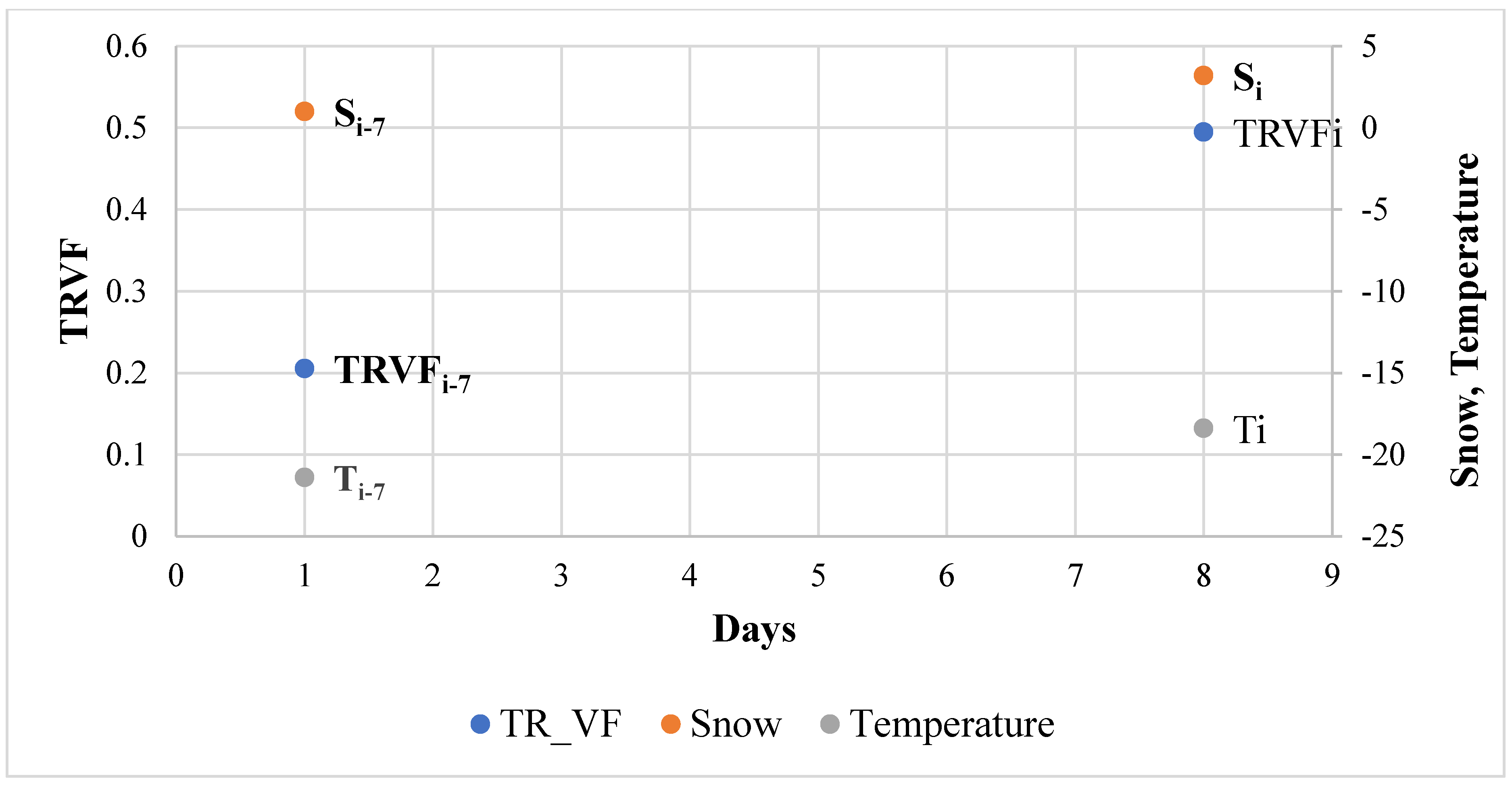
- Classification of snowy days based on changes in weather conditions from the same weekday in the previous week.
- MINE analysis on the obtained classified data.
- 1.
- Snow Difference:
- 2.
- Temperature Difference:
- 3.
- TRVF Difference:
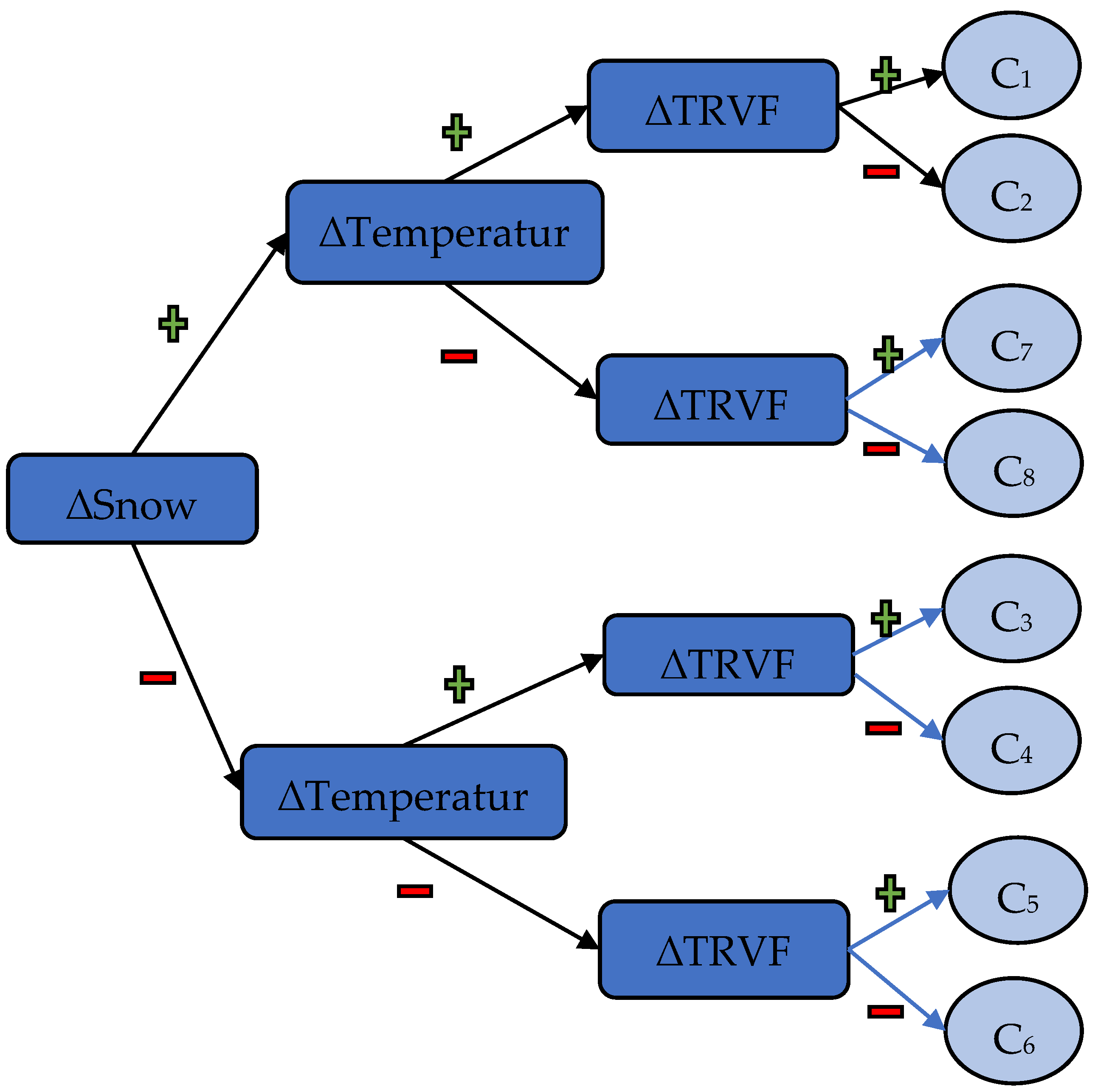
- C1Number of cases (days on which) when ∆Si > 0 (snowfall increases), ∆Ti > 0 (temperature increases) and ∆TRVFi > 0 (traffic count increases)
- C2Number of cases (days on which) when ∆Si > 0 (snowfall increases), ∆Ti > 0 (temperature increases) and ∆TRVFi < 0 (traffic count decreases)
- C3Number of cases (days on which) when ∆Si < 0 (snowfall decreases), ∆Ti > 0(temperature increases) and ∆TRVFi > 0 (traffic count increases)
- C4Number of cases (days on which) when ∆Si < 0 (snowfall decreases), ∆Ti > 0 (temperature increases) and ∆TRVFi < 0 (traffic count decreases)
- C5Number of cases (days on which) when ∆Si < 0 (snowfall decreases), ∆Ti < 0(temperature decreases) and ∆TRVFi > 0 (traffic count increases)
- C6Number of cases (days on which) when ∆Si < 0 (snowfall decreases), ∆Ti < 0 (temperature decreases) and ∆TRVFi < 0 (traffic decrease)
- C7Number of cases (days on which) when ∆Si > 0 (snowfall increases), ∆Ti < 0 (temperature decreases) and ∆TRVFi > 0 (traffic count increases)
- C8Number of cases (days on which) when ∆Si > 0 (snowfall increases), ∆Ti < 0 (temperature decreases) and ∆TRVFi < 0 (traffic count decreases)
- C9Number of cases for which, ∆Si = 0 or ∆Ti = 0
6. Results and Analysis
7. Discussion and Conclusions
Author Contributions
Funding
Conflicts of Interest
References
- Hassan, Y.A.; Barker, J.J. The impact of unseasonable or extreme weather on traffic activity within Lothian region, Scotland. J. Transp. Geogr. 1999, 7, 209–213. [Google Scholar] [CrossRef]
- Angel, M.; Sando, M.; Chimba, D.; Kwigizile, V. Effects of rain on traffic operations on florida freeways. J. Transp. Res. Board 2014, 2440. [Google Scholar] [CrossRef]
- Singhal, A.; Kamga, C. Impact of weather on urban transit ridership. Transp. Res. Part A Policy Pract. 2014, 69, 379–391. [Google Scholar] [CrossRef]
- Datla, S.; Sharma, S. Impact of cold and snow on temporal and spatial variations of highway traffic volumes. J. Transp. Geogr. 2008, 16, 358–372. [Google Scholar] [CrossRef]
- Knapp, K.K.; Smithson, L.D. Winter storm event volume impact analysis using multiple-source archived monitoring data. Transp. Res. Record 2000, 1700, 10–16. [Google Scholar] [CrossRef]
- Maze, T.H.; Crum, M.R.; Burchett, G. An Investigation of User Costs and Benefits of Winter Road Closures. 2005. Available online: http://lib.dr.iastate.edu/intrans_reports/21 (accessed on 20 October 2019).
- Pierce, D.; Short, J. Road closures and freight diversion: Analysis with empirical data. Transp. Res. Record 2012, 2269, 51–57. [Google Scholar] [CrossRef]
- Datla, S.; Sahu, P.; Roh, H.-J.; Sharma, S. A comprehensive analysis of the association of highway traffic with winter weather conditions. Procedia Soc. Behav. Sci. 2013, 104, 497–506. [Google Scholar] [CrossRef]
- Bardal, K.G. Impacts of adverse weather on arctic road transport. J. Transp. Geogr. 2017, 59, 49–58. [Google Scholar] [CrossRef]
- Roh, H.J.; Sharma, S.; Sahu, P.; Datla, S. Analysis and modeling of highway truck traffic volume variations during severe winter weather conditions in Canada. J. Mod. Transp. 2015, 23, 228–239. [Google Scholar] [CrossRef]
- Roh, H.J.; Sahu, P.; Sharma, S.; Datla, S.; Mehran, B. Statistical investigations of snowfall and temperature interaction with passenger car and truck traffic on primary highways in Canada. J. Cold Reg. Eng. 2016, 30. [Google Scholar] [CrossRef]
- Reshef, D.N.; Reshef, Y.A.; Finucane, H.K.; Grossman, S.R.; McVean, G.; Turnbaugh, P.J.; Lander, E.S.; Mitzenmacher, M.; Sabeti, P.C. Detecting novel associations in large data sets. Science 2011, 334, 1518–1524. [Google Scholar] [CrossRef] [PubMed]
- Keay, K.; Simmonds, I. The association of rainfall and other weather variables with road traffic volume in Melbourne, Australia. Accid. Anal. Prev. 2005, 37, 109–124. [Google Scholar] [CrossRef] [PubMed]
- Samba, D.; Park, B. Incorporating inclement weather impacts on traffic estimation and prediction. In Proceedings of the 18th ITS World Congress on Intelligent Transportation Systems, Orlando, FL, USA, 16–20 October 2011. [Google Scholar]
- Hanbali, R.M.; Kuemmel, D.A. Traffic Volume Reduction Due to Winter Storm Conditions; Transportation Research Record, No. 1387; Transportation Research Board of the National Academies: Washington, DC, USA, 1993; pp. 159–164. [Google Scholar]
- Maze, T.H.; Agarwal, M.; Burchett, G.D. Whether Weather Matters to Traffic Demand, Traffic Safety, and Traffic Operations and Flow; Transportation Research Record, No. 1948; Transportation Research Board of the National Academies: Washington, DC, USA, 2006; pp. 170–176. [Google Scholar] [CrossRef]
- Roh, H.J. Impacts of Snowfall, Low Temperatures, and Their Interaction on Passenger Car and Truck Traffic. Ph.D. Thesis, Department of Environmental Systems, University of Regina, Regina, SK, Canada, 2015. [Google Scholar]
- Omar, A.M.S.; Narula, S.; Rahman, M.A.A.; Pedrizzetti, G.; Raslan, H.; Rifaie, O.; Narula, J.; Sengupta, P.P. Precision phenotyping in heart failure and pattern clustering of ultrasound data for the assessment of diastolic dysfunction. JACC Cardiovasc. Imaging 2017, 2157. [Google Scholar] [CrossRef]
- Valenza, G.; Greco, A.; Gentili, C.; Lanata, A.; Sebastiani, L.; Menicucci, D.; Gemignani, A.; Scilingo, E.P. Combining electroencephalographic activity and instantaneous heart rate for assessing brain–heart dynamics during visual emotional elicitation in healthy subjects. Philos. Trans. R. Soc. Lond. A 2016, 374. [Google Scholar] [CrossRef]
- Zhouzhou, S.; Wei, Y. Creating and improving a closed loop: Design optimization and knowledge discovery in architecture. Int. J. Archit. Comput. 2015, 13, 123–142. [Google Scholar] [CrossRef]
- Available online: http://www.exploredata.net/Downloads/MINE-Application (accessed on 6 January 2017).
- Environment Canada (EC) (2010) Weather Office, Gatineau, Quebec, Canada. Available online: www.climate.weatheroffice.gc.ca/climateData/canada_e.html (accessed on 20 October 2016).
- Andrey, J.; Olley, R. Relationships between weather and road safety, past and future directions. Climatol. Bull. 1990, 24, 123–137. [Google Scholar]
- Environmental System Research Institute Inc. (ESRI) (2010) ArcGIS 10 Help Library: Geographic Information System (GIS); ArcGIS 10: Redlands, CA, USA, 2010. [Google Scholar]
- Roh, H.J. Developing cold region winter-weather traffic models and testing their temporal transferability and model specification. J. Cold Reg. Eng. 2019, 33. [Google Scholar] [CrossRef]
- Roh, H.J. Modelling chronic winter hazards as a function of precipitation and Temperature. Nat. Hazards 2020, 104. [Google Scholar] [CrossRef]
- Roh, H.J. Spatial transferability testing of dummy variable winter-weather model using traffic data collected from five geographically dispersed weigh-in-motion sites in Alberta highway networks. J. Transp. Eng. A Syst. 2020, 146. [Google Scholar] [CrossRef]
- Roh, H.J. Development of winter climatic hazard models on traffic volume and assessment of their performance with four types of model structures. Nat. Hazards Rev. 2020, 21. [Google Scholar] [CrossRef]
- Roh, H.J. Assessing the effect of snowfall and cold temperature on a commuter highway traffic volume using several layers of statistical methods. Transp. Eng. 2020, 2. [Google Scholar] [CrossRef]


| Researcher | Location | Year | Traffic Reduction Due to Rainfall | Traffic Reduction Due to Snow |
|---|---|---|---|---|
| Hassan and Barker [1] | Scotland | 1999 | 3% | 10% |
| Angel and Sando [2] | Florida | 2014 | 5.5–12.5% per hour along I-295 segment, 2.5–10.7% per hour along I-95 segment | -- |
| Datla and Sharma [4] | Alberta | 2008 | -- | Commuter roads—14%, Recreational roads—31% |
| Knapp and Smithson [5] | Iowa | 2000 | -- | 16% to 47% for different winter storms |
| Roh et al. [10] | Alberta | 2015–2020 | Average snowfall (<15cm) and Temperature greater than 25 °C do not affect truck traffic | |
| Keay and Simmonds [13] | Melbourne | 2005 | 1.35%—Winter, 2.11%—Spring | -- |
| Samba and Park [14] | Virginia, Minnesota | 2011 | 20% | 70% |
| Hanbali and Kuemmel [15] | Illinois, Minnesota, New York, Wisconsin | 1993 | -- | Light snow: 12%—Weekday, 25%—Weekends, Heavy Snow: 53%—Weekday, 56%—Weekends |
| Maze [16] | Iowa | 2006 | -- | Low wind speed and good visibility: 20%, High wind speed and poor visibility: 80% |
| Maximal Correlation Coefficient (MIC) | ||||
|---|---|---|---|---|
| 0.88 | 0.62 | 0.56 | 0.48 | |
| Relationship Type |  Added Noise Added Noise  | |||
| Line and Parabola |  |  |  |  |
| Two Lines |  |  |  |  |
| X |  |  |  |  |
| Ellipse |  |  |  |  |
| Sinusoid (Mixture of 3 signals) |  |  |  |  |
| Non co-existence |  |  |  |  |
| Site Name | Lanes | TAADT | Passenger Cars (%) | Trucks (%) | No. of Vehicle Records |
|---|---|---|---|---|---|
| Red Deer on Hwy 2—RD 3 | 4 | 4976 | 84 | 16 | 57,080,185 |
| Leduc on Hwy 2—LV 4 | 4 | 3964 | 83 | 17 | 44,386,644 |
| Leduc on Hwy 2A—LE 5 | 2 | 592 | 92 | 8 | 13,807,011 |
| Fort MacLeod on Hwy 3—FM 6 | 4 | 1075 | 85 | 15 | 12,835,403 |
| Edson Hwy on Hwy 16—ED 7 | 4 | 2358 | 68 | 32 | 13,350,824 |
| Villeneuve on Hwy 44—VI 8 | 2 | 2044 | 73 | 27 | 12,673,164 |
| Total Records | 154,133,231 | ||||
| Case | ∆Si | ∆Ti | ∆TRVFi |
|---|---|---|---|
| C1 | Increase | Increase | Increase |
| C2 | Increase | Increase | Decrease |
| C3 | Decrease | Increase | Increase |
| C4 | Decrease | Increase | Decrease |
| C5 | Decrease | Decrease | Increase |
| C6 | Decrease | Decrease | Decrease |
| C7 | Increase | Decrease | Increase |
| C8 | Increase | Decrease | Decrease |
| Highway | C1 | C2 | C3 | C4 | C5 | C6 | C7 | C8 | C9 |
|---|---|---|---|---|---|---|---|---|---|
| ED7 | 9 | 8 | 1 | 0 | 1 | 1 | 16 | 27 | 3 |
| FM6 | 20 | 10 | 1 | 1 | 6 | 4 | 45 | 41 | 2 |
| LE5 | 38 | 31 | 5 | 5 | 9 | 7 | 41 | 53 | 6 |
| LV4 | 36 | 33 | 7 | 3 | 9 | 7 | 31 | 63 | 6 |
| RD3 | 27 | 27 | 4 | 2 | 5 | 4 | 37 | 68 | 3 |
| VI8 | 33 | 21 | 5 | 4 | 6 | 6 | 25 | 59 | 7 |
| MIC (Strength) | MIC- ρ2 (Nonlinearity) | MAS (Non-Monotonicity) | MEV (Functionality) | MCN (Complexity) | Pearson Correlation (ρ) | Highway |
|---|---|---|---|---|---|---|
| 0.325 | 0.318 | 0.148 | 0.325 | 2.585 | 0.084 | ED7 |
| 0.300 | 0.287 | 0.091 | 0.300 | 3.000 | −0.115 | FM6 |
| 0.318 | 0.247 | 0.080 | 0.279 | 3.322 | −0.267 | LE5 |
| 0.412 | 0.147 | 0.072 | 0.367 | 3.585 | −0.515 | LV4 |
| 0.346 | 0.295 | 0.165 | 0.305 | 3.585 | −0.226 | RD3 |
| 0.266 | 0.206 | 0.042 | 0.238 | 3.585 | −0.245 | VI8 |
Publisher’s Note: MDPI stays neutral with regard to jurisdictional claims in published maps and institutional affiliations. |
© 2020 by the authors. Licensee MDPI, Basel, Switzerland. This article is an open access article distributed under the terms and conditions of the Creative Commons Attribution (CC BY) license (http://creativecommons.org/licenses/by/4.0/).
Share and Cite
Sahu, P.K.; Bayireddy, L.M.; Roh, H.-J. A New Approach to Exploring the Relationship between Weather Phenomenon and Truck Traffic Volume in the Cold Region Highway Network. Modelling 2020, 1, 122-133. https://doi.org/10.3390/modelling1020008
Sahu PK, Bayireddy LM, Roh H-J. A New Approach to Exploring the Relationship between Weather Phenomenon and Truck Traffic Volume in the Cold Region Highway Network. Modelling. 2020; 1(2):122-133. https://doi.org/10.3390/modelling1020008
Chicago/Turabian StyleSahu, Prasanta K., Leela Manas Bayireddy, and Hyuk-Jae Roh. 2020. "A New Approach to Exploring the Relationship between Weather Phenomenon and Truck Traffic Volume in the Cold Region Highway Network" Modelling 1, no. 2: 122-133. https://doi.org/10.3390/modelling1020008
APA StyleSahu, P. K., Bayireddy, L. M., & Roh, H.-J. (2020). A New Approach to Exploring the Relationship between Weather Phenomenon and Truck Traffic Volume in the Cold Region Highway Network. Modelling, 1(2), 122-133. https://doi.org/10.3390/modelling1020008