Does Eplet Load and Electrostatic Mismatch Score Matter in Kidney Transplantation? A Machine Learning Approach

Abstract

Background/Objectives: Kidney transplantation (KT) is the preferred treatment for end-stage renal disease (ESRD), offering improved quality of life, superior survival rates and lower economic burden. However, improving long-term kidney allograft survival post transplantation remains a significant challenge. HLA eplet matching has emerged as a promising strategy to minimize immunological risk and enhance long-term graft survival. Still, our understanding of HLA immunogenicity remains limited. This study aims to evaluate if Electrostatic mismatch score (EMS) and eplet mismatch (EpMM) are significant for predicting KT outcomes and their optimal cut-off values associated with improved graft survival. Methods: Our study analyzed over 10,000 kidney transplant records from the Scientific Registry of Transplant Recipients (SRTR) dataset using traditional survival analysis and machine learning (ML) techniques. The immunogenicity scores EMS and EpMM were calculated based on donor-recipient HLA molecular mismatches. Kaplan–Meier plots, Cox proportional hazards (CPH), random survival forests (RSF), and survival decision trees (SDT) were utilized in assessing the significance of EpMM and EMS in improving KT outcomes and their optimal cut-offs. Results: EpMM and EMS were found to be significant predictors of kidney graft survival. The optimal cutoff values for improved outcomes for EMS and EpMM were 11 and 7 respectively, beyond which graft failure risk increased. The RSF model was the best-performing model in KT outcome prediction (C-index = 0.6945, Brier score = 0.1460). Conclusions: EMS and EpMM were significant in the prediction of kidney transplantation outcomes at cutoffs of 11 and 7, respectively. Incorporating these measures in KT organ allocation strategies could improve long-term survival outcomes.

1. Introduction

Kidney transplantation (KT) is the optimal treatment for end-stage renal disease (ESRD) due to the superior patient survival and quality of life associated with it compared to kidney replacement therapy (dialysis) [1]. The US Health Resources and Services Administration maintains a national database of kidney patients showing that the demand for kidney transplants is continuously increasing, with approximately 100,000 people waiting for a transplant and nearly 3000 more added each month [2]. Despite more than 27,000 transplants being performed in 2023, 28,000 new patients were added to the waiting list in the same year [3] (Figure 1). The insufficient number of transplants performed results in tragic waiting list mortality, as about 17 people die daily while waiting, and others are removed from the waiting list due to deterioration of health. Also, a new patient joins the waiting list approximately every 10 min [2].

Despite significant progress in improving short-term outcomes of kidney transplantation, achieving long-term success remained stagnant over the last twenty years [4]. As a result, failure of existing kidney graft remains a single most significant factor contributing to the growing backlog of patients on the waiting list [2,5]. The short-term and long-term results of kidney transplantation are affected by a multitude of factors, including demographic [6], clinical [7], and immunological [8,9] covariates, and the accurate estimation of pre-transplant risk based on these factors is important for developing kidney donor allocation strategies [10].

Kidney transplant centers and organ procurement centers face a variety of challenges when developing their kidney donor allocation policy, including organ scarcity, high retransplantation costs, graft rejection, the risk of graft failure, and long waiting lists [11]. The development of accurate predictive models for long-term survival of kidney allografts is important to allow medical professionals and transplant stakeholders to develop better allocation strategies, as well as treatment plans for patients. As such, it is crucial to identify the predictive factors that impact the effectiveness of renal grafts and predict how long a graft of a given match will last.

While many clinical studies have examined the effects of both donor and recipient factors on graft survival, the interactions between them are complex and require further investigation. Existing statistical models such as Kaplan–Meier survival estimates and Cox proportional hazard regressions have limited ability to predict kidney graft outcomes [12,13,14]. Machine learning (ML) methods are an emerging approach with the potential to improve the prediction accuracy of kidney graft outcomes, offering a number of advantages in outcome prediction compared to traditional statistical models [15,16,17,18].

ML-based survival models offer two notable approaches for predicting the outcome of kidney transplantation: by partitioning post-transplant follow-up time into time intervals [17] or by stratifying the patient cohort by risk groups and forecasting the risk of adverse outcome within a particular time frame [18]. To address the high dimensionality problem in kidney transplant datasets, various feature selection techniques have been proposed. Some studies relied on expert opinions [15,19,20,21], while others employed univariate statistical tests [22].

Matching prospective donor–recipient pairs by Human Leukocyte Antigen (HLA) has been demonstrated to improve long-term allograft survival in multiple studies [23,24,25,26,27,28,29,30], however, less than 6% of transplants are fully antigenically matched by HLA in the United States. Diversity in HLA gene cluster together with overall shortage of donors makes it challenging to require HLA match for patients on the waiting list; however, recent studies show that a change in approach to quantifying HLA match may expand the possibilities for HLA matching without the need to increase donor numbers (REF). Alternative approaches to quantifying HLA mismatch by using the molecular HLA structure have been proposed [31]. This particular HLA mismatch quantitation system builds on the popular system created by Rene Duquesnoy in which immunogenic HLA molecule residues called eplets are deduced from the three-dimensional HLA protein structure and compared between donor and recipient [32]. The eplet mismatches (EpMMs) are complemented by the quantified physicochemical properties of HLA amino acids, contributing to the hydrophobic mismatch (HMS) and electrostatic mismatch (EMS).

In view of this, our study examines the significance of the eplet mismatch (EpMM) and electrostatic mismatch score (EMS) in KT survival. To investigate this, the study uses statistical, feature selection, and ML techniques to identify optimally not only the importance of these measures to survival but also the threshold values for these parameters that improve KT outcomes.

Our study specifically makes the following contributions:

• Investigates the significance of EpMM and EMS immunogenicity values in kidney transplant (KT) survival using both ML and traditional survival analysis methods.
• Finds the optimal cut-off values for the EMS and EpMM required to improve KT transplant outcomes, focusing on how immunogenicity mismatches affect the survival rates of transplants.

2. Materials and Methods

We collected and processed kidney transplant patient and donor data from the Scientific Registry of Transplant Recipients (SRTR), collected characteristics represented by patient confounder variables, imputed novel characteristics, and constructed models to analyze the survival of the kidney graft over time and to determine and evaluate the characteristics that contribute to the survival of the kidney graft. Two ML models were used in our prediction modeling. The models were evaluated mainly using the concordance index (C index) and the Brier score. All statistical analyses for this study were performed in Python using the lifelines library and sci-kit survival.

2.1. Data Description

This study used data from the Scientific Registry of Transplant Recipients (SRTR). The SRTR data system includes data on all donor, wait-listed candidates, and transplant recipients in the U.S., submitted by members of the Organ Procurement and Transplantation Network (OPTN). The U.S. Department of Health and Human Services provides oversight of the activities of the OPTN and SRTR contractors.

The dataset for this study comprised more than 10,000 kidney transplants over approximately 30 years (1990 to 2022), with more than 100 characteristics.

To expand our analysis and explore additional factors that could contribute to determining kidney graft survival, we included a comprehensive set of characteristics beyond those recommended by experts in previous studies. This approach allowed us to identify potential predictors that may have been overlooked by earlier research. This study specifically focused on incorporating newly generated immunogenicity features (EpMM and EMS) not used in similar previous studies to uncover possible new insights that affect kidney graft survival.

For the purposes of this survival analysis, graft loss was defined to encompass any of the following: kidney graft failure, resumption of maintenance dialysis, retransplantation or listed for retransplantation, and death with a functioning graft. This is referred to as All-Cause Graft Failure (ACGF). In this study, the time to event referred to the duration from transplant to kidney graft loss as defined above.

2.2. Data Preparation

The data compiled from the SRTR data initially consisted of over 10,000 records (rows) and more than 100 features. To ensure data quality and relevance, a data cleaning process was conducted. This involved removing various columns containing irrelevant or personal identification information such as recipient ID, donor ID, Hospital ID, patient’s citizenship, patient’s working status, and other confidential details.

Furthermore, redundant features that provided similar information such as height and weight were eliminated. These features were reflected in a derived variable called Body Mass Index (BMI). By removing these duplicate features, the dataset was streamlined and made more concise for subsequent analyses. Furthermore, records with more than 80% missing data, which accounted for less than 1% of the dataset, were excluded from the analysis [33]. This decision was made to reduce noise, as such records lack sufficient information and could degrade model performance. The exclusion had minimal impact on the sample size, which remained large enough to support robust conclusions. The remaining incomplete data were addressed through the utilization of single imputation technique [34,35]. Also, the characteristics of excluded data were checked to ensure that they did not disproportionately belong to specific patient subgroups that would otherwise affect the conclusions of the study.

As part of the data pre-processing steps in calculating the immunogenicity scores, donor/recipient HLA was converted from low resolution (serological) to high resolution (molecular) using the relevant medical histo-compability information, after which we performed immunogenicity calculations. This process is described in more detail in Section 2.3. This process also added new variables, EMS and EpMM, to that of the original SRTR data.

Table 1. List of Features.

Feature Description	Data Type
Previous kidney transplant	Categorical
Donor age	Continuous
Recipient age	Continuous
Donor BMI	Continuous
Recipient BMI	Continuous
Donor history of hypertension	Categorical
Recipient history of hypertension	Categorical
Donor race	Categorical
Recipient race	Categorical
Electrostatic mismatch score (EMS)	Continuous
Eplet load mismatch (EpMM)	Continuous
Donor hepatitis C virus	Categorical
Donor history of diabetes	Categorical
Recipient history of diabetes	Categorical
Donor creatinine level	Continuous
Angina and coronary artery disease status	Categorical
Donor gender	Categorical
Recipient gender	Categorical
Serum creatinine	Continuous
History of cancer	Categorical
History of cigarette use	Categorical
Recipient age at transplant	Continuous
Transplant center	Categorical
EBV serology status	Categorical
Donor relation to patient	Categorical
Most recent serum PRA (%)	Continuous
HIV serology status	Categorical
Kidney produced > 40 mL of urine in first 24 h	Categorical
Dialysis status	Categorical
Initial peak PRA (max of peak)	Continuous
Most-recent peak PRA (max of peak)	Continuous
Previous malignancy status	Categorical
Most recent serum creatinine	Continuous
Graft functional status	Continuous
Pretransplant dialysis status	Categorical
Kidney(s) received on ice or pump	Categorical
Warm ischemic time	Categorical
Cold ischemic time	Categorical

contains a list of some of the features used in our experiments, along with their corresponding descriptions.

2.3. Immunogenicity Imputation

For this study, immunogenicity was quantified based on the EMS and EpMM load. The EpMM score was calculated based on the methodology described in [36]. This process involved converting all donor/recipient HLA from low resolution (serological) to high resolution (molecular) using the relevant histocompatibility information from the joined SRTR data based on the HaploStats algorithm [37]. This was followed by mapping each donor allele to its corresponding set of known eplets through a structured internal database using the HLAMatchmaker algorithm [32], which catalogs the specific eplets associated with each allele. This process yielded a comprehensive index of all eplets present in the HLA alleles of the donor. Identical steps were conducted for the recipient to produce their eplet list. Subsequently, a comparison of the two sets (donor versus recipient) identified the eplet mismatches (AbvMismatches) between both.

Next, using the computer algorithm outlined in [36], the EMS was calculated by first converting the donor and recipient HLA types from low-resolution serological to high-resolution molecular typings based on the Cambridge HLA Immunogenicity algorithm approach [38,39]. These produced high-resolution typings which provided detailed physicochemical profiles including the electrostatic charge. EMS was then calculated by quantifying HLA disparities across the relevant HLA regions based on their electrostatic charges.

It is worth highlighting that the computer algorithm outlined in [36] used for computing the EMS builds upon an original computer algorithm that has been validated in previous studies, as documented in [38,39]. The original algorithm [38,39], which consists of spreadsheet-based applications, was adapted in [36] to create a Python-based implementation, which we utilized for our analysis, since our analysis was conducted with Python. Sampled results from the adapted Python algorithm were the same as those from the original algorithms.

2.4. Identifying the Optimal Cut-Off Values for EpMM and EMS

To the best of the authors’ knowledge, no prior studies have rigorously determined the optimal cut-off values needed to improve kidney transplant outcomes for EpMM and EMS. As such, the optimal cut-off points for EpMM and EMS are determined through a rigorous evaluation process. First, the model’s ability to rank patients at high versus low risk of kidney graft failure was assessed using various binning thresholds for the EpMM and EMS. The C-index of the survival models CPH, random survival forests (RSFs), and survival decision trees (SDT) was utilized in this evaluation. Secondly, these findings were further validated using the Kaplan–Meier method, which analyzed the survival differences between the cut-off groups. The statistical significance of these differences was confirmed by the log-rank test. The minimum p-value approach, signifying the most significant survival difference between groups, was used in selecting our best cutoffs [40,41].

2.5. Feature Selection and Engineering

Categorical features were transformed into several dummy features using one-hot encoding to make them compatible with the models used. To avoid issues of multicollinearity, where two or more predictor variables were highly correlated, one level of each categorical variable was dropped [42]. This allowed the model to estimate the effect of each level relative to the dropped level, which served as the reference category.

To streamline the feature space, optimize model prediction, and determine the most relevant features for our models, a series of univariate CPH models was constructed to screen out potentially significant variables, following the guidelines recommended in Collett [43] using a cut-off significance level of 0.10. Subsequently, using these features, a CPH multivariate analysis was performed using a combination of backward and forward selection techniques to identify the influencing factors to kidney graft survival at a statistically significant level of 0.05 (p-value = 0.05) Guyon and Elisseeff [44]. The univariate Cox model and CPH multivariate analysis (using a combination of backward and forward selection techniques) were preferred due to its strength in providing interpretable hazard ratios, enabling understanding of variable relationships. Interpretability is a key requirement in clinical settings, as practitioners need clear insights into the contribution of individual variables at each step of our analysis.

RSFs and SDTs were also used to calculate permutation-based feature importance scores to assess the relative importance of these covariates to kidney transplant survival rates.

Lastly, for the purpose of easy clinical applicability, five models (CPH, Lasso, RSF, SDT, and DeepSurv) were fitted by including only covariates that were found to have significant association and of clinical importance to KG survival.

To ascertain optimal binning for categorical variables in the study, domain experts were engaged to ensure the logical grouping of categories. Additionally, we implemented performance-based binning, which involved a systematic evaluation of how various bin configurations influenced our models’ performance. Furthermore, to improve the power of the analysis, the log-rank test was employed to determine which categories had significantly different survival rates for the binning of our categorical features [45].

Censoring was addressed through the use of right-censored survival models. Patients who did not experience graft failure or death by the end of the study period were considered right-censored at the time of their last follow-up. Similarly, patients lost to follow-up before experiencing the event were right-censored at the time of their last known follow-up. The Cox proportional hazards model, Kaplan–Meier survival curves, and machine learning models (random survival forests and survival decision trees) inherently handled right-censored data.

2.6. Statistical Models

In addition to Kaplan–Meier (KM) curves, this study employed two traditional statistical models. KM curves are commonly used in survival analysis to estimate the survival function of a population or a group of individuals over time [46]. The survival function represents the probability that an individual will survive past a certain time point.

Numerous studies have utilized KM curves effectively to examine the general survival rates of kidney transplant recipients [47,48,49]. The KM curves for this study were constructed using the lifelines libraries [50]. A KM curve is a non-parametric estimator.

The KM curves fell short in evaluating the effect and significance of the explanatory variables in kidney graft survival. This can be achieved by employing Cox Proportional Hazard (CPH) modeling. The CPH model is a semi-parametric model that makes no assumption regarding the underlying distribution of the survival function [51]. The key assumption that underpins the CPH model is the proportional hazards assumption. In this study, the lifelines proportional hazard test module was used to check the validity of the proportional hazards assumption. The CPH model defines a hazard function, $h(t,X)$, as [51]:

$$h(t,X)=h_0\left(t\right)exp\sum _{i=1}^{\tau }{\beta }_i{X}_i$$

(1)

where $h_0\left(t\right)$ is the baseline hazard function; ${\beta }_i$ denotes the regression coefficients; and X denotes the vector of predictor variables which are being modeled to predict the sample’s hazard. The “partial” likelihood method is used in estimating the regression coefficients of the CPH model. The partial likelihood, L, for estimation is approximated by the following equation [52]:

$$L={\pi }_{i=1}^{n_d}{\displaystyle \frac{exp\left(s_i^T\beta \right)}{{\left[{\sum }_{j\in R\left(t_i\right)}exp\left(X_j^T\beta \right)\right]}^{d_i}}}$$

(2)

where $s_i$ denotes the sum of covariates of samples observed to fail at time $t_i$; $R\left(t_i\right)$ is the set of samples at risk just prior to $t_i$, referred to as the risk set. The maximum likelihood estimate (MLE) of $\beta$ ($\widehat{\beta }$) is obtained by maximizing Equation (2) with the aid of the Newton–Raphson iteration technique [53], which utilizes the first and second derivatives of Equation (2) [51].

Penalized Cox regression models were also utilized, which are an extension of the standard Cox proportional hazards regression model. These models incorporate a penalty term on the regression coefficients to shrink them towards zero, thereby reducing overfitting and improving model generalizability [54]. L1 (Lasso) and L2 (ridge) penalties are some of the different types of penalty functions that can be used [54]. Penalized Cox regression models are particularly effective in handling high-dimensional data with a large number of potential predictor variables. They enable the simultaneous estimation of coefficients and variable selection [54]. For this study a Cox proportional hazard regression model with lasso regularization was used.

2.7. Machine Learning Models

In this study, three non-parametric ML-based survival models were applied to our survival data. These models included random survival forest, survival decision tree, and DeepSurv (using NN).

A survival decision tree (SDT) is a decision tree-based method that can handle survival data. It extends the standard decision tree by incorporating time-to-event information [55,56]. The splitting rules are chosen to minimize a splitting criterion such as the log-rank statistic or the Gini index [55,56]. In our study, the log-rank splitting rule [57] was employed to assess the quality of splits in the SDT models. SDT has demonstrated strong predictive capabilities for time-to-event outcomes in various domains, including medical research.

An RSF is a collection of decision trees used for survival analysis. By building each tree on a different bootstrap sample of the original training data and randomly selecting a subset of features and thresholds at each node, an RSF ensures that the individual trees are not correlated. The predictions are then formed by combining the predictions of all the trees in the ensemble [57,58]. It has been widely used to predict survival data.

DeepSurv is a deep neural survival method based on the Cox proportional hazards that was developed in 2018 for modeling interactions between a patient’s covariates and treatment effectiveness [59]. Our study incorporated DeepSurv due to its distinction as one of the limited deep learning techniques applicable to survival analysis. It demonstrates comparable or superior performance against alternative methods in analyzing survival data, effectively handling both linear and nonlinear covariate effects [59].

The dataset was randomly split into a training set and test set in a 7:3 ratio, respectively, to allow for a robust evaluation of the models’ performance and their ability to generalize to unseen data. To avoid overfitting and sampling bias that may affect the classification results, all models were trained using a 5-fold cross-validation approach. We optimized hyper-parameters using a grid-search approach.

C-indices were used as primary and Brier scores were used as secondary metrics of model performance in this study. The advantage of the C-index is it takes into account the ordering of predicted and actual survival times, which is important for survival analysis [60], while the Brier score is a valuable metric of model calibration [61,62].

3. Results

In this section, we present the results considering the significance of the EpMM and EMS in KT survival, including their optimal cut-off values required to improve KT outcomes.

3.1. Kidney Graft Survival by Donor Type and Immunogenicity Threshold

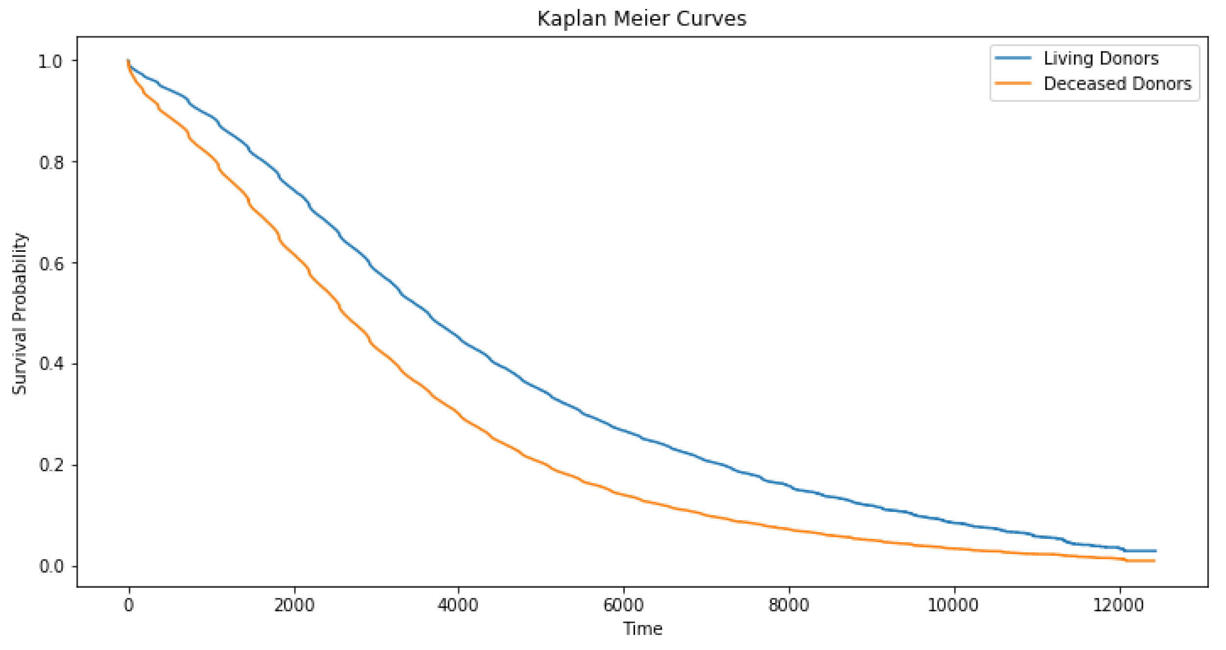
Median graft survival was around 7 years for deceased donor and 10 years for living donor recipients (Figure 2), with a significant decline in survival rates between days 2000 and 6000 in deceased compared to living donor recipients. This was consistent with the previously reported advantage of living donor transplantation (

Table 2. Table showing KPM survival probabilities among KG transplant patients involving living and deceased donors.

Time (in Days)	Survival Probability (Living Donors)	Survival Probability (Deceased Donors)
1000	0.8889	0.8100
2000	0.7433	0.6164
3000	0.5828	0.4304
4000	0.4509	0.2999
5000	0.3463	0.2031
6000	0.2662	0.1389
7000	0.2066	0.0984
8000	0.1567	0.0708
9000	0.1179	0.0494
10,000	0.0835	0.0328
11,000	0.0567	0.0219

).

Figure 3 illustrates the C-index scores for the survival models (CPH, RSF, SDT) as EMS binning thresholds vary. Initially, when the EMS was categorized into intervals of zero to eight versus greater than eight, the model demonstrated a consistently high C-index, indicating robust discriminatory performance over time. As we progressively included higher EMS values in bin (up to EMS 11), the model’s ability to distinguish between high-risk and low-risk subjects remains steady (C-index between 0.64 and 0.66). However, when the threshold included EMS values higher than 11, there was a noticeable decline in the model’s ability to discriminate between high-risk and low-risk subjects. The stability of the C-index between an EMS of 8 and 11 suggests the potential benefit of utilizing these thresholds for categorization.

Subsequently, the survival distributions of these cutoffs were compared using Kaplan–Meier plots and log-rank tests. The results are shown in

Table 3. Table showing the comparison of the survival distributions across various cutoffs using the log-rank test (EMS).

Cutoffs	Log-Rank Test
8	0.0127
9	0.0058
10	0.0032
11	0.0024
12	0.1370
13	0.1869
14	0.2051

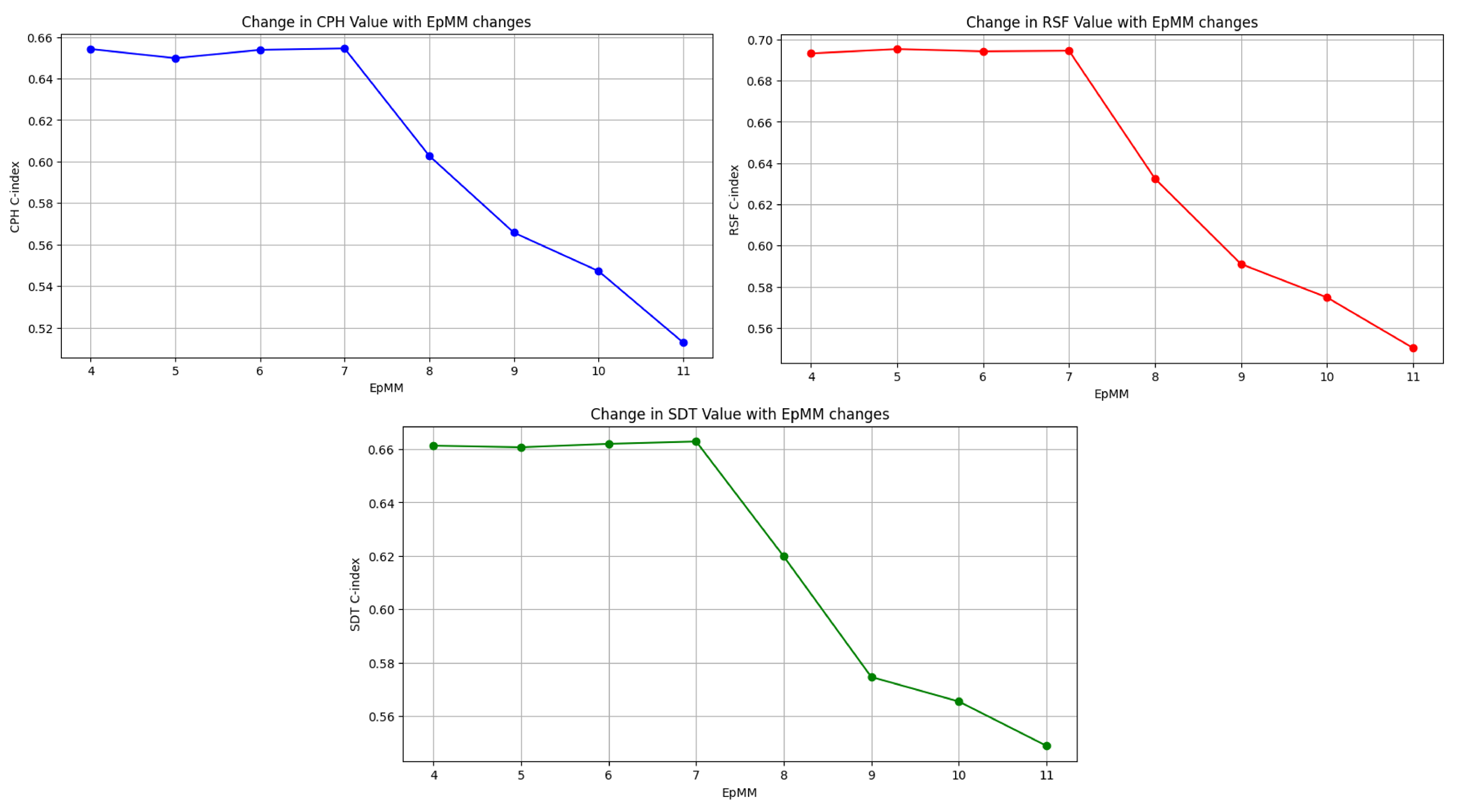
. Notably, the minimum p-value, signifying the most significant survival difference between groups, was observed for a cutoff of 11 (p-value = 0.0024). Hence, 11 was identified as the optimal cutoff for EMS categorization. Similar analyses conducted for the EpMM (shown in Figure 4 and

Table 4. Table showing the comparison of the survival distributions across various cut-offs using the log-rank test (EpMM).

Cutoffs	Log-Rank Test
4	0.0291
5	0.0046
6	0.0019
7	0.0003
8	0.0815
9	0.1228
10	0.1924
11	0.1683

) resulted in the identification of an optimal cutoff of seven for the EpMM.

3.2. Analysis of Prediction Performance of Models

Results from the multivariate Cox regression analysis (

Table 5. Table summary of covariates significantly impacting graft survival in kidney transplants: hazard ratios from Cox proportional hazards model.

Covariates	Coef	HR	CI	p-Value
Rec age (<60)	−0.3996	0.6706	(−0.4576, −0.3417)	<0.0001
Rec BMI (<30)	−0.0669	0.9353	(−0.1088, −0.0249)	0.0018
Can. race (blacks)	0.2213	1.2477	(0.1304, 0.3122)	<0.001
EpMM (>7)	0.2920	1.3391	(0.2502, 0.3339)	<0.0005
Don. rel. to rec (non bio.)	0.3328	1.3949	(0.0807, 0.5849)	0.0097
Previous TX (yes)	0.3624	1.4368	(0.3132, 0.4116)	<0.0005
Peak PRA	0.1482	1.1597	(0.0924, 0.2040)	<0.0001
EMS (>11)	0.1664	1.1811	(0.0762, 0.2566)	0.0003

) showed the EpMM and EMS had a statistically significant impact on graft survival of kidney transplants (p-value < 0.05). This finding is further supported by the permutation feature importance scores derived from the RSF and SDT models, which quantified the relative importance of each attribute (

Table 6. Table showing feature importance scores from RSF and SDT models.

Cut-Offs	Log-Rank Test
RSF
Previous TX	0.0713
EpMM	0.0379
EMS	0.0169
Rec BMI	0.0152
Rec age	0.0131
Don. rel. to Rec	0.0079
Can. race	0.0071
Peak PRA	0.0016
SDT
Previous TX	0.0621
EpMM	0.0244
Rec age	0.0172
EMS	0.0159
Can. race	0.0138
Don. rel. to Rec	0.0049
Peak PRA	0.0034
Rec BMI	0.0031

). For example, the permutation feature importance score of the EpMM from the RSF analysis was 0.04. This score implies that if its relationship to survival time was removed, the C-index would drop on average by 0.04 points, which indicates its essential role in predicting graft survival. Other important features influencing KT graft survival per our results were a candidate’s previous transplant status, recipient BMI, recipient age at the time of transplantation, donor relation to patient, candidate race, and most-recent peak PRA (Table 5 and Table 6).

Table 7. Table showing prediction performance of models.

Model	C-Index	IBS
Semi-Parametric
CPH	0.6545	0.1568
Lasso(pen = 0.01)	0.6551	0.1565
ML
RSF	0.6945	0.1460
SDT	0.6629	0.2927
DeepSurv (using NN)	0.6821	0.1138

provides a summary of the performance of our final models fitted by including the optimal EpMM and EMS cutoffs determined. The best-performing model overall was the random forest algorithm (C-index = 0.6945, Brier score = 0.1460). When examining our findings in the context of previous studies on kidney graft survival, it is worth noting that the C-index of our random forest model was approximately 70%, surpassing the benchmark value of 0.655 for kidney survival analysis using the SRTR dataset, which is the highest value we found in any published paper [63]. Thus, including these immunogenicity measures (EpMM and EMS) at the established thresholds in our models led to better KT predictions. The proportional hazard test indicated the proportional hazards assumption was not violated (p-value > 0.05).

4. Discussion

Kidney allograft survival has remained depressingly low over the last two decades, with median survival for deceased donor kidneys still hovering around 10–12 years [4]. Understanding the role of molecular HLA matching and involvement of physicochemical mismatch and eplet mismatch scoring in long-term post-transplant outcomes is important for improving allograft survival in the future [64]. However, traditional statistical methods for evaluating transplantation outcome, such as Kaplan–Meier survival estimates and Cox proportional hazard modeling have their limitations, making it important to explore novel machine learning strategies for studying kidney allograft survival. The experiments performed within this study yielded significant insights into kidney transplant (KT) outcomes by analyzing graft survival across donor types and exploring the predictive power of key immunogenicity metrics, EpMM and EMS.

Our work demonstrated that EMS thresholds between 8 and 11 provided stable and robust discrimination between high-risk and low-risk patients, while thresholds beyond 11 led to diminished predictive accuracy. Similarly, the optimal EpMM cutoff was identified as seven, with this value demonstrating the most significant stratification of survival outcomes.

Multivariate Cox regression and feature importance analyses supported the critical role of the EpMM and EMS in predicting KT survival, alongside other factors such as BMI, recipient age, and donor relationship. The random forest model emerged as the best-performing algorithm, achieving a C-index of 0.6945, which exceeded benchmarks from prior studies and highlighted the advantage of integrating these immunogenicity measures alongside ML methods. These findings underscore the practical utility of EpMM and EMS thresholds in enhancing KT survival predictions and provide a framework for refining clinical decision-making to optimize long-term outcomes.

A key limitation of our current study is the restricted access to external kidney transplant data due to confidentiality concerns and the sensitive nature of patient health information in almost all national transplant databases worldwide. These restrictions make it difficult to obtain external data from different countries or transplant centers. Despite this, the dataset used in this study represents the most comprehensive and diverse dataset for kidney transplantation in the United States, enabling our analysis to be conducted and validated on a broad and varied population through cross-validation to reduce the risk of overfitting to specific centers or regional characteristics. Despite these measures, we recognize the importance of external validation to confirm the broader applicability of the identified thresholds. Furthermore, the minimum p-value method is susceptible to arbitrary threshold selection and reproducibility issues. Therefore, validating our findings using independent datasets from transplant centers in different countries or regions is essential to ensure their generalizability beyond the U.S. population.

In the future, our findings will be further investigated and may lead to additional insights that lengthen the survival of KT patients. Options for further investigation include:

• The development of a pioneering multi-state analysis model to assess the effects of the EMS and EpMM on influencing transitions between the kidney transplant progression states of transplant, graft loss, retransplant and death;
• Recognizing the importance of external validation, future works include plans to engage international transplant centers and seek the necessary permissions to access external datasets for future studies. Validation with data from regions outside the U.S. will allow us to test the reproducibility and robustness of the cut-off thresholds identified in this study across the world.
• Conduct sensitivity analyses to evaluate the robustness of these thresholds across various patient subgroups (e.g, age, race, BMI, previous transplants, early vs. late graft loss scenarios etc.).
• Investigate the use of interaction terms (e.g., EpMM and recipient age, or EMS and donor-recipient relationship, etc.) to identify and validate complex relationships among these variables. Future research could also explore interactions between immunosuppressive therapy, EpMM, and EMS, provided that detailed information on patients’ immunosuppressive regimens becomes available, as these data are currently lacking in our study.

5. Conclusions

Our study assessed the impact of novel immunogenicity features, the EMS and EpMM, on kidney graft survival using both conventional and machine learning methods over a 30-year time frame, while also identifying the critical factors impacting such survival outcomes.

Our study identified the optimal cut-off value for the EpMM and EMS to enhance kidney transplant (KT) outcomes as 7 and 11, respectively. The study also found the EMS and EpMM significantly influenced the outcome of kidney transplants. Additional factors significantly impacting kidney graft survival were the recipient’s prior transplant history, time on pretransplant dialysis, the recipient’s BMI, age at transplantation, the donor’s relationship to the recipient, the recipient’s race, and most-recent peak PRA. These features can be considered as good prognostic factors that could lead to better kidney graft outcomes. Furthermore, our study showed that machine learning could provide accurate alternatives to traditional techniques for kidney transplant survival analysis.

We conclude that the EMS and EpMM significantly influence kidney transplant outcomes, and including these immunogenicity measures at the established thresholds in our models leads to better KT predictions. We recommend for kidney exchange programs to use donor–recipient pairings with an EpMM and EMS below the thresholds of 7 and 11, respectively, to potentially prolong kidney graft survival and eventually optimize kidney matching processes.

The text continues here (Figure 2 and Table 2).

References

- Badrouchi, S.; Ahmed, A.; Bacha, M.M.; Abderrahim, E.; Abdallah, T.B. A machine learning framework for predicting long-term graft survival after kidney transplantation. Expert Syst. Appl. 2021, 182, 115235. [Google Scholar] [CrossRef]
- HRSA, H.R. Services. Administration. Organ Donation Statistics. 2022. Available online: https://www.organdonor.gov/learn/organ-donation-statistics (accessed on 8 November 2024).
- HRSA. National Data. 2024. Available online: https://data.hrsa.gov/ (accessed on 20 November 2024).
- Poggio, E.D.; Augustine, J.J.; Arrigain, S.; Brennan, D.C.; Schold, J.D. Long-term kidney transplant graft survival—Making progress when most needed. Am. J. Transplant. 2021, 21, 2824–2832. [Google Scholar] [CrossRef]
- Rees, M.A.; Kopke, J.E.; Pelletier, R.P.; Segev, D.L.; Rutter, M.E.; Fabrega, A.J.; Rogers, J.; Pankewycz, O.G.; Hiller, J.; Roth, A.E.; et al. A nonsimultaneous, extended, altruistic-donor chain. N. Engl. J. Med. 2009, 360, 1096–1101. [Google Scholar] [CrossRef] [PubMed]
- Nautiyal, A.; Bagchi, S.; Bansal, S.B. Gender and kidney transplantation. Front. Nephrol. 2024, 4, 1360856. [Google Scholar] [CrossRef]
- Ahmadpoor, P.; Seifi, B.; Zoghy, Z.; Bakhshi, E.; Dalili, N.; Poorrezagholi, F.; Nafar, M. Time-varying covariates and risk factors for graft loss in kidney transplantation. Transplant. Proc. 2020, 52, 3069–3073. [Google Scholar] [CrossRef] [PubMed]
- Steiner, T.; Boehme, C.; Wolf, G.; Schubert, J.; Ott, U. Impact of immunologic and nonimmunologic variables on long-term outcome after kidney transplantation. Transplant. Proc. 2009, 41, 2521–2523. [Google Scholar] [CrossRef]
- Tambur, A.R.; Kosmoliaptsis, V.; Claas, F.H.; Mannon, R.B.; Nickerson, P.; Naesens, M. Significance of HLA-DQ in kidney transplantation: Time to reevaluate human leukocyte antigen–matching priorities to improve transplant outcomes? An expert review and recommendations. Kidney Int. 2021, 100, 1012–1022. [Google Scholar] [CrossRef]
- Adler, J.T.; Husain, S.A.; King, K.L.; Mohan, S. Greater complexity and monitoring of the new kidney allocation system: Implications and unintended consequences of concentric circle kidney allocation on network complexity. Am. J. Transplant. 2021, 21, 2007–2013. [Google Scholar] [CrossRef]
- Saidi, R.; Kenari, S.H. Challenges of organ shortage for transplantation: Solutions and opportunities. Int. J. Organ Transplant. Med. 2014, 5, 87. [Google Scholar]
- Vinson, A.J.; Kiberd, B.A.; Davis, R.B.; Tennankore, K.K. Nonimmunologic donor-recipient pairing, HLA matching, and graft loss in deceased donor kidney transplantation. Transplant. Direct 2019, 5, e414. [Google Scholar] [CrossRef]
- Young, A.; Knoll, G.A.; McArthur, E.; Dixon, S.N.; Garg, A.X.; Lok, C.E.; Lam, N.N.; Kim, S.J. Is the kidney donor risk index a useful tool in non-US patients? Can. J. Kidney Health Dis. 2018, 5, 2054358118791148. [Google Scholar] [CrossRef] [PubMed]
- Rao, P.S.; Schaubel, D.E.; Guidinger, M.K.; Andreoni, K.A.; Wolfe, R.A.; Merion, R.M.; Port, F.K.; Sung, R.S. A comprehensive risk quantification score for deceased donor kidneys: The kidney donor risk index. Transplantation 2009, 88, 231–236. [Google Scholar] [CrossRef] [PubMed]
- Brown, T.S.; Elster, E.A.; Stevens, K.; Graybill, J.C.; Gillern, S.; Phinney, S.; Salifu, M.O.; Jindal, R.M. Bayesian modeling of pretransplant variables accurately predicts kidney graft survival. Am. J. Nephrol. 2012, 36, 561–569. [Google Scholar] [CrossRef] [PubMed]
- Ravindhran, B.; Chandak, P.; Schafer, N.; Kundalia, K.; Hwang, W.; Antoniadis, S.; Haroon, U.; Zakri, R.H. Machine learning models in predicting graft survival in kidney transplantation: Meta-analysis. BJS Open 2023, 7, zrad011. [Google Scholar] [CrossRef]
- Naqvi, S.A.A.; Tennankore, K.; Vinson, A.; Roy, P.C.; Abidi, S.S.R. Predicting kidney graft survival using machine learning methods: Prediction model development and feature significance analysis study. J. Med. Internet Res. 2021, 23, e26843. [Google Scholar] [CrossRef]
- Topuz, K.; Zengul, F.D.; Dag, A.; Almehmi, A.; Yildirim, M.B. Predicting graft survival among kidney transplant recipients: A Bayesian decision support model. Decis. Support Syst. 2018, 106, 97–109. [Google Scholar] [CrossRef]
- Nematollahi, M.; Akbari, R.; Nikeghbalian, S.; Salehnasab, C. Classification models to predict survival of kidney transplant recipients using two intelligent techniques of data mining and logistic regression. Int. J. Organ Transplant. Med. 2017, 8, 119. [Google Scholar]
- Maple-Brown, L.J.; Hughes, J.T.; Lawton, P.D.; Jones, G.R.; Ellis, A.G.; Drabsch, K.; Brown, A.D.; Cass, A.; Hoy, W.E.; MacIsaac, R.J.; et al. Accurate assessment of kidney function in indigenous Australians: The estimated GFR study. Am. J. Kidney Dis. 2012, 60, 680–682. [Google Scholar] [CrossRef]
- Lin, R.S.; Horn, S.D.; Hurdle, J.F.; Goldfarb-Rumyantzev, A.S. Single and multiple time-point prediction models in kidney transplant outcomes. J. Biomed. Inform. 2008, 41, 944–952. [Google Scholar] [CrossRef]
- Akl, A.; Ismail, A.M.; Ghoneim, M. Prediction of graft survival of living-donor kidney transplantation: Nomograms or artificial neural networks? Transplantation 2008, 86, 1401–1406. [Google Scholar] [CrossRef]
- Husain, S.A.; King, K.L.; Sanichar, N.; Crew, R.J.; Schold, J.D.; Mohan, S. Association between donor-recipient biological relationship and allograft outcomes after living donor kidney transplant. JAMA Netw. Open 2021, 4, e215718. [Google Scholar] [CrossRef] [PubMed]
- Stapleton, C.P.; Lord, G.M.; Conlon, P.J.; Cavalleri, G.L.; UK and Ireland Renal Transplant Consortium. The relationship between donor-recipient genetic distance and long-term kidney transplant outcome. HRB Open Res. 2020, 3, 47. [Google Scholar] [CrossRef]
- Hernandez-Fuentes, M.P.; Franklin, C.; Rebollo-Mesa, I.; Mollon, J.; Delaney, F.; Perucha, E.; Stapleton, C.; Borrows, R.; Byrne, C.; Cavalleri, G.; et al. Long-and short-term outcomes in renal allografts with deceased donors: A large recipient and donor genome-wide association study. Am. J. Transplant. 2018, 18, 1370–1379. [Google Scholar] [CrossRef]
- Farouk, S.; Zhang, Z.; Menon, M.C. Non-HLA donor–recipient mismatches in kidney transplantation—A stone left unturned. Am. J. Transplant. 2020, 20, 19–24. [Google Scholar] [CrossRef]
- Santori, G.; Barocci, S.; Fontana, I.; Bertocchi, M.; Tagliamacco, A.; Biticchi, R.; Valente, U.; Nocera, A. Kidney transplantation from living donors genetically related or unrelated to the recipients: A single-center analysis. Transplant. Proc. 2012, 44, 1892–1896. [Google Scholar] [CrossRef]
- Arthur, V.L.; Guan, W.; Loza, B.l.; Keating, B.; Chen, J. Joint testing of donor and recipient genetic matching scores and recipient genotype has robust power for finding genes associated with transplant outcomes. Genet. Epidemiol. 2020, 44, 893–907. [Google Scholar] [CrossRef] [PubMed]
- Miles, C.D.; Schaubel, D.E.; Liu, D.; Port, F.K.; Rao, P.S. The role of donor-recipient relationship in long-term outcomes of living donor renal transplantation. Transplantation 2008, 85, 1483–1488. [Google Scholar] [CrossRef] [PubMed]
- Zhang, Z.; Menon, M.C.; Zhang, W.; Stahl, E.; Loza, B.L.; Rosales, I.A.; Yi, Z.; Banu, K.; Garzon, F.; Sun, Z.; et al. Genome-wide non-HLA donor-recipient genetic differences influence renal allograft survival via early allograft fibrosis. Kidney Int. 2020, 98, 758–768. [Google Scholar] [CrossRef]
- Kosmoliaptsis, V.; Sharples, L.D.; Chaudhry, A.; Johnson, R.J.; Fuggle, S.V.; Halsall, D.J.; Bradley, J.A.; Taylor, C.J. HLA class I amino acid sequence-based matching after interlocus subtraction and long-term outcome after deceased donor kidney transplantation. Hum. Immunol. 2010, 71, 851–856. [Google Scholar] [CrossRef]
- Duquesnoy, R.J. HLAMatchmaker: A molecularly based algorithm for histocompatibility determination. I. Description of the algorithm. Hum. Immunol. 2002, 63, 339–352. [Google Scholar] [CrossRef]
- Little, R.J.; Rubin, D.B. Statistical Analysis with Missing Data; John Wiley & Sons: Hoboken, NJ, USA, 2019; Volume 793. [Google Scholar]
- Graham, J.; Olchowski, A.; Gilreath, T. Review: A gentle introduction to imputation of missing values. Prev. Sci. 2007, 8, 206–213. [Google Scholar] [CrossRef] [PubMed]
- Graham, J.W. Missing data analysis: Making it work in the real world. Annu. Rev. Psychol. 2009, 60, 549–576. [Google Scholar] [CrossRef] [PubMed]
- Mastrocinque, M. Epitope-based Re-matching of Donor-Recipient Pairs for Kidney Graft Allocation. Master’s Thesis, Bowling Green State University, Bowling Green, OH, USA, 2021. [Google Scholar]
- Maiers, M.; Gragert, L.; Klitz, W. High-resolution HLA alleles and haplotypes in the United States population. Hum. Immunol. 2007, 68, 779–788. [Google Scholar] [CrossRef]
- Kosmoliaptsis, V.; Sharples, L.D.; Chaudhry, A.N.; Halsall, D.J.; Bradley, J.A.; Taylor, C.J. Predicting HLA class II alloantigen immunogenicity from the number and physiochemical properties of amino acid polymorphisms. Transplantation 2011, 91, 183–190. [Google Scholar] [CrossRef] [PubMed]
- Kosmoliaptsis, V.; Chaudhry, A.N.; Sharples, L.D.; Halsall, D.J.; Dafforn, T.R.; Bradley, J.A.; Taylor, C.J. Predicting HLA class I alloantigen immunogenicity from the number and physiochemical properties of amino acid polymorphisms. Transplantation 2009, 88, 791–798. [Google Scholar] [CrossRef]
- Hasford, J.; Pfirrmann, M.; Hehlmann, R.; Allan, N.C.; Baccarani, M.; Kluin-Nelemans, J.C.; Alimena, G.; Steegmann, J.L.; Ansari, H. A new prognostic score for survival of patients with chronic myeloid leukemia treated with interferon alfa Writing Committee for the Collaborative CML Prognostic Factors Project Group. JNCI J. Natl. Cancer Inst. 1998, 90, 850–859. [Google Scholar] [CrossRef]
- Motzer, R.J.; Mazumdar, M.; Bacik, J.; Berg, W.; Amsterdam, A.; Ferrara, J. Survival and prognostic stratification of 670 patients with advanced renal cell carcinoma. J. Clin. Oncol. 1999, 17, 2530–2540. [Google Scholar] [CrossRef]
- Fox, J. Applied Regression Analysis and Generalized Linear Models; Sage Publications: Thousand Oaks, CA, USA, 2015. [Google Scholar]
- Collett, D. Modelling Survival Data in Medical Research; CRC Press: Boca Raton, FL, USA, 2023. [Google Scholar]
- Guyon, I.; Elisseeff, A. An introduction to variable and feature selection. J. Mach. Learn. Res. 2003, 3, 1157–1182. [Google Scholar]
- Breslow, N.E. The design and analysis of cohort studies. Stat. Methods Cancer Res. 1987, 2, 1–174. [Google Scholar]
- Kaplan, E.L.; Meier, P. Nonparametric estimation from incomplete observations. J. Am. Stat. Assoc. 1958, 53, 457–481. [Google Scholar] [CrossRef]
- Lee, D.; Kim, H.Y.; Lee, J.H.; Sin, Y.H.; Kim, J.K.; Oh, J.S. Long-term survival analysis of kidney transplant recipients receiving mizoribine as a maintenance immunosuppressant: A single-center study. Transplant. Proc. 2019, 51, 2637–2642. [Google Scholar] [CrossRef]
- Coemans, M.; Süsal, C.; Döhler, B.; Anglicheau, D.; Giral, M.; Bestard, O.; Legendre, C.; Emonds, M.P.; Kuypers, D.; Molenberghs, G.; et al. Analyses of the short-and long-term graft survival after kidney transplantation in Europe between 1986 and 2015. Kidney Int. 2018, 94, 964–973. [Google Scholar] [CrossRef] [PubMed]
- Rich, J.T.; Neely, J.G.; Paniello, R.C.; Voelker, C.C.; Nussenbaum, B.; Wang, E.W. A practical guide to understanding Kaplan-Meier curves. Otolaryngol. Head Neck Surg. 2010, 143, 331–336. [Google Scholar] [CrossRef]
- Davidson-Pilon, C. lifelines: Survival analysis in Python. J. Open Source Softw. 2019, 4, 1317. [Google Scholar] [CrossRef]
- Showkat, B.; Singh, D. Perceiving moisture damage of asphalt mixes containing RAP using survival analysis based on Kaplan-Meier estimator and Cox proportional hazards model. Constr. Build. Mater. 2022, 320, 126249. [Google Scholar] [CrossRef]
- Klein, J.P.; Moeschberger, M.L. Survival Analysis: Techniques for Censored and Truncated Data; Springer: Berlin/Heidelberg, Germany, 2003; Volume 1230. [Google Scholar]
- Ypma, T.J. Historical development of the Newton–Raphson method. SIAM Rev. 1995, 37, 531–551. [Google Scholar] [CrossRef]
- Tibshirani, R. The lasso method for variable selection in the Cox model. Stat. Med. 1997, 16, 385–395. [Google Scholar] [CrossRef]
- Bou-Hamad, I.; Larocque, D.; Ben-Ameur, H. A review of survival trees. Statist. Surv. 2011, 5, 44–71. [Google Scholar] [CrossRef]
- Hothorn, T.; Hornik, K.; Zeileis, A. Unbiased recursive partitioning: A conditional inference framework. J. Comput. Graph. Stat. 2006, 15, 651–674. [Google Scholar] [CrossRef]
- Pölsterl, S. scikit-survival: A Library for Time-to-Event Analysis Built on Top of scikit-learn. J. Mach. Learn. Res. 2020, 21, 8747–8752. [Google Scholar]
- Ishwaran, H.; Kogalur, U.B.; Blackstone, E.H.; Lauer, M.S. Random survival forests 2008. Ann. Appl. Stat. 2008, 2, 841–860. [Google Scholar] [CrossRef]
- Katzman, J.L.; Shaham, U.; Cloninger, A.; Bates, J.; Jiang, T.; Kluger, Y. DeepSurv: Personalized treatment recommender system using a Cox proportional hazards deep neural network. BMC Med. Res. Methodol. 2018, 18, 1–12. [Google Scholar] [CrossRef] [PubMed]
- Wolbers, M.; Blanche, P.; Koller, M.T.; Witteman, J.C.; Gerds, T.A. Concordance for prognostic models with competing risks. Biostatistics 2014, 15, 526–539. [Google Scholar] [CrossRef] [PubMed]
- Brier, G.W. Verification of forecasts expressed in terms of probability. Mon. Weather. Rev. 1950, 78, 24. [Google Scholar] [CrossRef]
- Graf, E.; Schmoor, C.; Sauerbrei, W.; Schumacher, M. Assessment and comparison of prognostic classification schemes for survival data. Stat. Med. 1999, 18, 2529–2545. [Google Scholar] [CrossRef]
- Luck, M.; Sylvain, T.; Cardinal, H.; Lodi, A.; Bengio, Y. Deep learning for patient-specific kidney graft survival analysis. arXiv 2017, arXiv:1705.10245. [Google Scholar]
- Bekbolsynov, D.; Mierzejewska, B.; Borucka, J.; Liwski, R.S.; Greenshields, A.L.; Breidenbach, J.; Gehring, B.; Leonard-Murali, S.; Khuder, S.A.; Rees, M.; et al. Low hydrophobic mismatch scores calculated for HLA-A/B/DR/DQ loci improve kidney allograft survival. Front. Immunol. 2020, 11, 580752. [Google Scholar] [CrossRef]