Data-Driven Inverse Design of Hybrid Waveguide Gratings Using Reflection Spectra via Tandem Networks and Conditional VAEs

Abstract

This study presents a data-driven inverse design approach for one-dimensional hybrid waveguide gratings using full reflection spectra across the visible range and a complete span of incident angles. Traditionally, designing such structures to achieve specific optical responses relies on parameter sweeps and iterative simulations which are computationally expensive, time-consuming, and often inefficient. To overcome this, we generated a comprehensive dataset using rigorous coupled-wave analysis (RCWA) simulations and trained two machine learning models: a deterministic tandem network and a generative conditional Variational Autoencoder (cVAE). Both models were trained on noisy reflection spectra to mimic real-world measurements. They both predict structural parameters accurately on clean and noisy data. On clean data, the mean absolute error (MAE) for silver thickness and grating period is below 1 nm. For the dielectric layer, the error is about 13–15 nm. When noise is added, the Tandem network performs best with low to moderate noise. The cVAE, however, stays more stable under high noise conditions. At $\sigma =0.3$, the cVAE model reliably predicts the silver thickness and grating period, with MAEs below 6 nm. The main error comes from the dielectric thickness. Sensitivity analysis of reflection spectra confirms this trend. The reflection is least sensitive to the dielectric thickness, while silver thickness and grating period dominate. This analysis provides physical insight for waveguide design as well in which, accurate control of silver thickness and grating period is far more critical than small errors in dielectric thickness. In general, our approach enables rapid prediction of structural parameters of hybrid waveguide gratings from reflection spectra. This reduces design time and reliance on complex microscopic measurements, with potential applications in sensing, communication, and integrated photonics.

1. Introduction

Waveguide gratings are well known for their ability to couple free-space modes to guided waveguide modes forming guided-mode resonances (GMRs). The spectral position and quality factor (Q-factor) of the GMRs are dependent on the geometrical parameters of the structure, such as the grating period, waveguide thickness, and refractive index contrast [1]. Such resonances are also highly sensitive to changes in the surrounding environment and can be used to detect changes in the refractive index of the surrounding medium, which is useful in sensing applications such as sensors for chemical and biological detections [2], biosensing applications (e.g., [3,4,5]), bio-imaging (e.g., [6,7]), strain sensing, and strain measurement applications (e.g., [8,9]). GMRs are also highly sensitive to the wavelength and angle of incident light [1], making them suitable for filtering applications (e.g., [10,11,12,13,14,15]) and optical communications (e.g., [16]).

Waveguide-based structures can support different types of mode coupling phenomena depending on the materials and geometries involved. In purely dielectric systems, photonic-photonic mode coupling can occur, which shows the highest Q-factors and is widely used in integrated photonics [17,18]. Multilayer dielectric structures, e.g., 1D photonic crystals, can also support Bloch surface waves, which exhibit strong field confinement and surface-localized propagation [19]. Additionally, in waveguides containing metal films, photonic-plasmonic coupling can arise. The guided modes—surface plasmon polaritons (SPPs)—enable strong field localization, which is particularly promising for sensing applications due to a high sensitivity to refractive index changes close to the metal surface. At very thin metal films and gratings two SPPs can hybridize [20,21], while in general SPPs and photonic transverse magnetic (TM) modes can hybridize as well [22,23]. The resulting modes can combine the benefits of high Q-factors and high sensitivity.

In this work, we focus on hybrid plasmonic photonic waveguide gratings, where a dielectric slab waveguide is combined with a thin metallic grating. The geometry enables the maximum complexity of hybrid TM modes within the waveguide, so the GMRs prediction is difficult. On the other hand, it provides sufficient propagation losses to limit the sharpness of the GMRs. This way, a suitable spectral resolution with regard to energy and momentum can be defined that ensures no GMRs are missed by the simulations.

For material selection, silver is chosen due to its well-known strong support of surface plasmon polaritons in the visible spectrum [20,24]. As the dielectric layer, we chose the transparent polymer OrmoCore. OrmoCore is a commercially available polymer suitable for low-loss waveguides. The combination of silver and OrmoCore layers forms a robust platform for hybrid waveguide gratings [23,25,26]. The OrmoCore–silver grating stack was placed on top of a glass substrate.

While the effective refractive index of purely dielectric modes cannot exceed the index of the dielectric core [1 $<n_{eff}<$ 1.58], the results presented in Supporting Information reveal multiple mode solutions that exhibit high real parts of the effective refractive index, reaching values as large as 1.954 at 580 nm, indicating the hybrid nature of the associated modes.

In our study, we concentrate on three primary geometrical parameters: the silver thickness, the dielectric (OrmoCore) thickness, and the grating period. These parameters were selected based on their dominant influence on the position, sharpness, and number of GMRs observed in the reflection spectra. Although other design spaces may involve different materials or additional parameters, such as grating dimensions or multilayer configurations, our chosen parameter set strikes a balance between physical interpretability and complexity, making it ideal for training and evaluating inverse design models.

Machine Learning (ML) has emerged as a tool in photonics, supporting a wide range of tasks from material characterization and real-time process monitoring to image-based diagnostics and design optimization. A particularly promising application area is inverse design, where the goal is to identify structural parameters that yield desired optical properties (e.g., [27,28,29]). Instead of relying solely on computationally expensive parameter sweeps, ML models can learn the complex mapping between optical responses and structural configurations, thereby accelerating the design process. This strategy has proven effective in various domains, such as photonic crystals [30], metamaterials [31], resonators [32], and quantum nanophotonics [33], with applications ranging from optical computing and light manipulation to sensing and optical communication systems.

State-of-the-Art and Motivation

The core idea behind ML-based inverse design is to decrease the expenses associated with generating new data by substituting simulations or experiments with AI models. However, inverse design comes with intrinsic challenges. A key issue is that most inverse design problems are considered ill-posed, meaning that different structures may lead to the same output, and multiple viable solutions exist [34,35].

As a result, a direct inverse neural network that attempts to learn a one-to-many mapping from desired properties to design parameters can struggle to produce stable or representative predictions. This is due to the inherent ambiguity in the inverse mapping, which can lead the model to average over multiple valid solutions or to become biased toward certain regions of the design space [34,35,36].

Numerous studies to date have endeavored to address the problem of non-uniqueness inherent in the input-output relationship of the inverse design models. For instance, it has been suggested to introduce appropriate constraints, such as limiting the design space or projecting it to a low-dimensional space, to establish a well-defined problem [37,38].

One approach involved segmenting the training dataset into distinct groups. They partitioned the overall training data into groups based on the derivative of the forward model’s output with respect to its input, to ensure each group exhibited a one-to-one mapping from response to design [34]. This segmentation aimed to reduce ambiguity in the inverse problem. For each of these distinct groups of data, an individual inverse neural network model was trained. The final prediction was obtained by feeding the input into all trained inverse models, passing their outputs through the trained forward model, and selecting the model whose output closely matched the input. This strategy resulted in higher prediction accuracy compared to training a single inverse model on the entire dataset. However, the challenge remains in properly clustering the data, especially for more complex or high-dimensional design spaces.

To address the ill-posed nature of the inverse design problem, a tandem architecture was proposed that combines a pre-trained forward model with a trainable inverse model. Hence, the model learns by minimizing the error between the predicted and input optical responses [35]. Nevertheless, using a tandem network, only one of the several possible design configurations is predicted for the desired output, and the remaining alternatives are intentionally dismissed to minimize the training loss. Consequently, the tandem network potentially neglects other alternatives that could be more feasible, cost-effective, or convenient in terms of fabrication.

Generative AI models, such as a conditional Variational Autoencoder (cVAE) [39] enable tackling the ill-posed issue and can generate multiple valid design candidates for a given target response (e.g., [40]). Instead of converging to a single solution, the cVAE maps the same desired optical spectrum to a distribution of structurally distinct yet physically consistent parameter sets. However, due to the single-modal normal distribution assumption in standard cVAE frameworks, the diversity of generated structural parameters is often limited in practice (e.g., [28]).

Alternatively, conditional Generative Adversarial Network (cGAN) [41] have been shown to provide higher diversity and flexibility in inverse design tasks. Nevertheless, this increased diversity often comes at the cost of reduced accuracy, making cGAN less suitable for applications where precise prediction of structural parameters is critical (e.g., [28]).

In this work, we address the inverse design of hybrid waveguide gratings based on their reflection spectra using two different ML approaches, Tandem Network and cVAE. The remainder of this paper is organized as follows: Section 2 describes the simulation setup and the overall methodology, including the dimensionality reduction of data and the applied ML approaches. Section 3 outlines the evaluation procedure and explains how prediction accuracy, robustness, and errors are assessed. In Section 4 and Section 5, we present and discuss the detailed results and conclusions based on our findings.

2. Materials and Methods

To investigate the optical properties of the proposed hybrid waveguide gratings, accurate modeling of light–matter interactions at the nanoscale is essential to predict device performance and guide the inverse design process. For this project, Rigorous Coupled-Wave Analysis (RCWA) simulations were utilized to compute the reflection of the zero-order TM reflected wave for 1D periodic nanostructures under non-conical incidence [42,43].

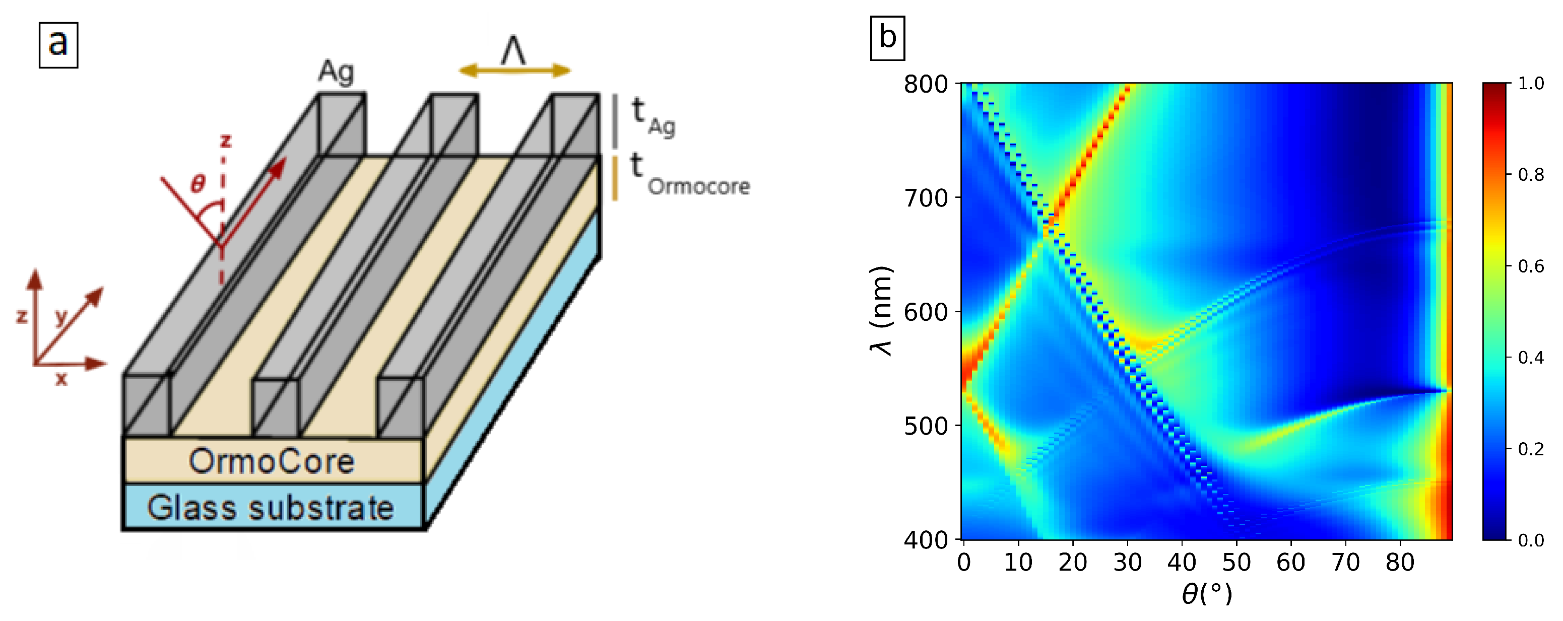
In our study, the inputs to the simulations include the structural parameters of the device, such as the material of the dielectric or metal layers, their corresponding thicknesses, the periodic distances in the x-direction, and the size of the grating. A schematic of the structure used in this research is presented in Figure 1a. As can be seen, the structure used in this study is a one-dimensional grating made of silver, placed atop a dielectric slab waveguide.

OrmoCore with a refractive index in the range of 1.54 to 1.58 and normal dispersion in the visible range given by the Cauchy formula:

$$n\left(\lambda \right)=A+{\displaystyle \frac{B}{{\lambda }^2}}+{\displaystyle \frac{C}{{\lambda }^4}}$$

(1)

with A = 1.53, B = 8000 nm², and $C=0.70{\mathrm{nm}}^4$. For silver, we used the optical constants reported by Palik [44], which account for both the real and imaginary parts of the refractive index.

The values for the silver thickness, $t_{Ag}$, the dielectric slab thickness, $t_{OrmoCore}$, and the grating period, $\mathrm{\Lambda }$, are randomly selected within specified ranges: 10–100 nm for $t_{Ag}$, 0–1500 nm for the $t_{OrmoCore}$, and 280–550 nm for the $\mathrm{\Lambda }$. The structure is supported by a glass substrate. The thickness of the glass substrate is considered infinitely thick. Each combination of these parameters is unique and non-repetitive. In total, 15,000 simulations were performed to sufficiently cover the 3D design space while balancing computational cost and model training requirements. In each case, the filling factor of the grating is 0.5, due to easy fabrication. To balance the computational efficiency and precision of the RCWA simulations, we retained 10 Fourier orders per side (21 in total) in all calculations.

Although these parameter ranges were chosen to broadly explore the design space, relevant fabrication constraints are considered. In particular, silver layers thinner than 10 nm are known to form discontinuous, island-like structures rather than uniform films, making them impractical to fabricate reliably [45,46]. Therefore, ultra-thin silver layers were excluded from the simulation range. Concerning OrmoCore layers, layer thicknesses less than 80 nm are challenging to produce using standard fabrication processes. Nevertheless, this lower range was included in the simulations in order to fully investigate the influence of dielectric thickness on device performance.

The incident light is a TM-polarized plane wave, and the output, as it is shown in Figure 1b, represents the zero-order TM reflection for different angles, $\theta$, and wavelengths, $\lambda$, of the incident light, where $\theta$ is the angle between the incident wave and the z-axis (perpendicular to the plane), varied between 0 and 89 degrees. The simulations were performed for wavelengths from the spectral range of interest, 400–800 nm.

To address the one-to-many nature of the inverse design problem with a focus on accuracy, we have implemented two approaches: a Tandem network [35] and a cVAE [39].

Before training the models, an autoencoder is used to extract low-dimensional latent representations from the reflection data, simplifying the learning process and reducing computational complexity.

2.1. Dimensionality Reduction of Reflection Data Using Autoencoders

In this work, a convolutional autoencoder (AE) is trained to compress high dimensional reflection spectra of 2D matrices of size 401 × 90 into a compact latent representation of size 128 without losing important information. The encoder maps each spectrum into a lower dimensional representation. Simultaneously, the decoder is trained to reconstruct the original reflection spectra from this latent space, ensuring minimal information loss during compression [47].

After training, only the encoder is used to convert each reflection matrix into its corresponding latent vector. This conversion reduces the dimensionality of the data, which simplifies the input for the subsequent forward and tandem networks, as well as the cVAE, reduces computational complexity, and improves learning efficiency, while still preserving critical spectral features.

We trained the autoencoder as a denoising model by adding Additive Gaussian Noise (AGN) to each input reflection matrix during training. AGN was chosen as it closely approximates the type of noise typically observed in reflection measurements from real samples. The standard deviation, $\sigma$, of the noise was randomly sampled from a uniform range [0, 0.1] for each sample in a batch and regenerated at every training iteration. The network was trained to reconstruct the original clean input from noisy data, forming a denoising autoencoder (e.g., [48]). As a result, the latent vectors extracted from the denoising autoencoder, which are later used as inputs to subsequent models, ensure that subsequent models are resilient to the noise and fluctuations typical of real-world measurements. Additional details of the autoencoder model architecture are provided in Appendix A.1.

While AGN adequately represents random detector fluctuations, real measurement data can also be affected by colored noises. Colored noises are the stochastic noise characterized by its power spectrum caused by systematic effects such as source drifts or environmental instabilities. In this study, white noise was considered during training. However, the trained models were additionally evaluated with colored noise applied to the reflection spectra as well. For more information, see Section S3 of the Supplementary Information.

2.2. Tandem Network

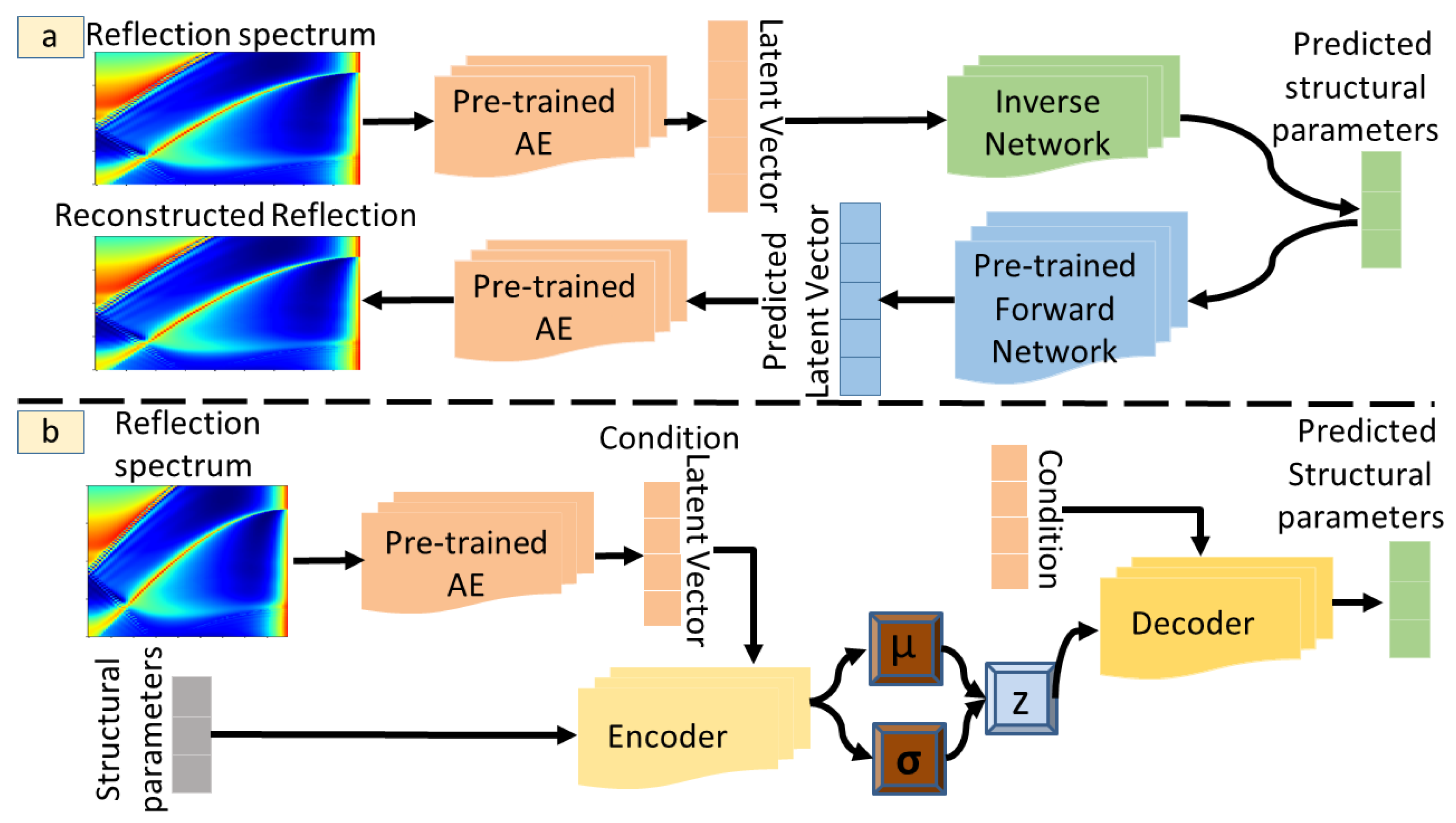
The Tandem network combines Forward and Inverse Neural Networks, as shown schematically in Figure 2a.

Prior to training the Tandem Network, the high-dimensional reflection spectra are compressed using the pre-trained AE (see Section 2.1). This step transforms each reflection matrix into a lower-dimensional latent vector, which retains essential spectral features. These latent vectors are then used as the target outputs for training the forward model and as the input data for the inverse model in the Tandem Network.

The forward model, which maps structural parameters to their corresponding optical responses, is first trained independently using supervised learning on a large dataset of simulated design-response pairs. Once trained, its weights are frozen. Here, we train a Forward Neural Network (FNN) to predict the lower-dimensional latent representations of the reflection spectra obtained from the AE, from given structural parameters using the mean squared error (MSE) as the loss function for the FNN:

$$L_{FNN}={\displaystyle \frac{1}{N}}\sum _{i=1}^N{(y_i-g\left(x_i\right))}^2$$

(2)

where N is the number of training samples, $y_i$ is the latent representations of the reflection spectra for the i-th data point, and $g\left(x_i\right)$ is the FNN’s predicted latent representation of reflection spectra for the structure $x_i$.

The FNN is then integrated into a joint architecture with an Inverse Neural Network (INN), which maps the latent representation of the target spectra to candidate structural parameters. During training, the predicted structures from the INN are passed through the fixed FNN, and the loss is computed between the resulting and target latent representation of the spectra. This Tandem loss is used to update only the weights of the INN, ensuring physically consistent inverse predictions [35].

$$L_{Tandem}={\displaystyle \frac{1}{N}}\sum _{i=1}^N{(y_i-g\left(f\left(y_i\right)\right))}^2$$

(3)

where $f\left(y_i\right)$ is the predicted structure for the latent vector $y_i$, and $g\left(f\left(y_i\right)\right)$ is the latent representation of the reflection spectra predicted by the pre-trained FNN. As can be seen, the tandem loss directly depends on the output of the pretrained forward model g. Since only the inverse model f is updated during the training, the accuracy of the INN’s predictions is inherently constrained by the quality of g. This approach also ensures that the INN converges to a solution consistent with the FNN’s predictions, thereby tackling the ill-posed problem. Further details of the model architecture are provided in Appendix A.2.

2.3. Conditional Variational Autoencoder (cVAE)

In order to predict the three structural parameters from reflection spectra, we trained a cVAE. In this model, both the encoder and decoder are conditioned on the reflection data to ensure that the generated structural parameters comply with the physical constraints dictated by the input spectrum [39].

As an auxiliary condition, $\mathbf{c}$, the model uses low-dimensional latent vectors extracted from the reflection data by the pre-trained autoencoder (see Section 2.1). By incorporating this condition into both the encoder and decoder, the cVAE learns a latent space, $\mathbf{z}$, that captures the variability in the structural parameters while remaining consistent with the latent representation of the reflection spectrum.

The overall architecture, illustrated in Figure 2b, consists of an encoder, a latent space, and a decoder. The encoder processes the structural parameters along with the condition $\mathbf{c}$ and maps them into a probabilistic latent space characterized by a mean and variance. The decoder then reconstructs the structural parameters by combining a sampled latent vector with the same condition $\mathbf{c}$, ensuring that the predicted structures are physically consistent with the input reflection data. Additional model architecture details are provided in Appendix A.3.

The model is trained by optimizing a loss function that consists of two terms: a reconstruction loss, which ensures the predicted structural parameters closely match the ground truth, and a Kullback–Leibler (KL) divergence term, which regularizes the latent space to follow a standard normal distribution. Formally, the loss is:

$$L(\varphi ,\theta )=\underset{\mathrm{Reconstruction}\mathrm{Loss}}{\underbrace{-{\mathbb{E}}_{q_{\varphi }(\mathbf{z}\mid \mathbf{x},\mathbf{c})}\left[log{p}_{\theta }(\mathbf{x}\mid \mathbf{z},\mathbf{c})\right]}}+\underset{\mathrm{KL}\mathrm{Divergence}}{\underbrace{D_{\mathrm{KL}}\left(q_{\varphi }(\mathbf{z}\mid \mathbf{x},\mathbf{c})\Vert p(\mathbf{z}\mid \mathbf{c})\right)}}$$

(4)

where $q_{\varphi }(\mathbf{z}\mid \mathbf{x},\mathbf{c})$ is the encoder that approximates the posterior distribution of the latent variable $\mathbf{z}$ given both the input $\mathbf{x}$ and the condition $\mathbf{c}$. $p_{\theta }(\mathbf{x}\mid \mathbf{z},\mathbf{c})$ is the decoder that reconstructs $\mathbf{x}$ from both $\mathbf{z}$ and $\mathbf{c}$. $p(\mathbf{z}\mid \mathbf{c})$ is the prior distribution of the latent variable conditioned on $\mathbf{c}$.

Figure 2. Schematic structure of the combination of the autoencoder for dimensionality reduction with (a) the Tandem Network and (b) the cVAE. The reflection spectra are shown as color maps and the colored blocks denote different neural-network components.

Figure 2. Schematic structure of the combination of the autoencoder for dimensionality reduction with (a) the Tandem Network and (b) the cVAE. The reflection spectra are shown as color maps and the colored blocks denote different neural-network components.

3. Results

To evaluate our proposed approaches, we first assess the accuracy of the dimensionality reduction using the AE. Since the AE forms the foundation for subsequent models by compressing complex reflection spectra into compact latent representations, it is essential to ensure that this compression preserves the essential spectral information. In particular, the denoising capability of the AE plays a crucial role in enhancing model robustness against measurement noise.

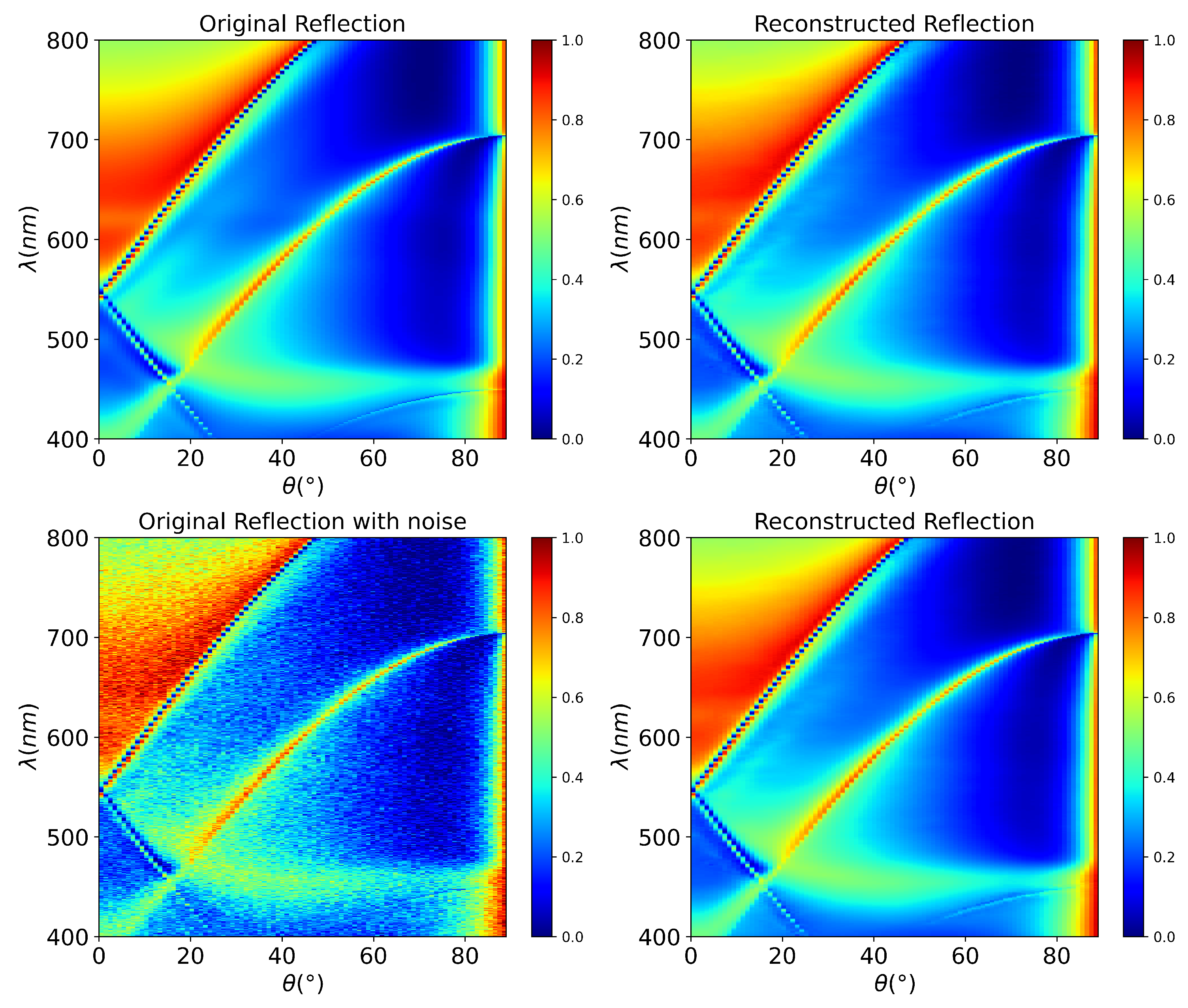
To quantitatively assess the performance of the trained AE, we computed mean squared error (MSE) and mean absolute error (MAE) between the original and reconstructed reflection spectra for the test dataset. For the noise-free test dataset, the AE achieved an average MSE of $8.9\times {10}^{-5}$ and MAE of $4.7\times {10}^{-3}$, with only a negligible increase to $9.7\times {10}^{-5}$ and $5.0\times {10}^{-3}$ under noisy inputs with constant $\sigma =0.1$. Given that the reflection values range between 0 and 1, these error values confirm that the AE reliably compresses and reconstructs the high-dimensional data for noise-free and noisy inputs. In addition, a visual comparison of a reflection spectra from test dataset and its reconstruction using the trained AE is shown in Figure 3. The reconstruction of a noisy reflection spectrum is shown in the second row of Figure 3.

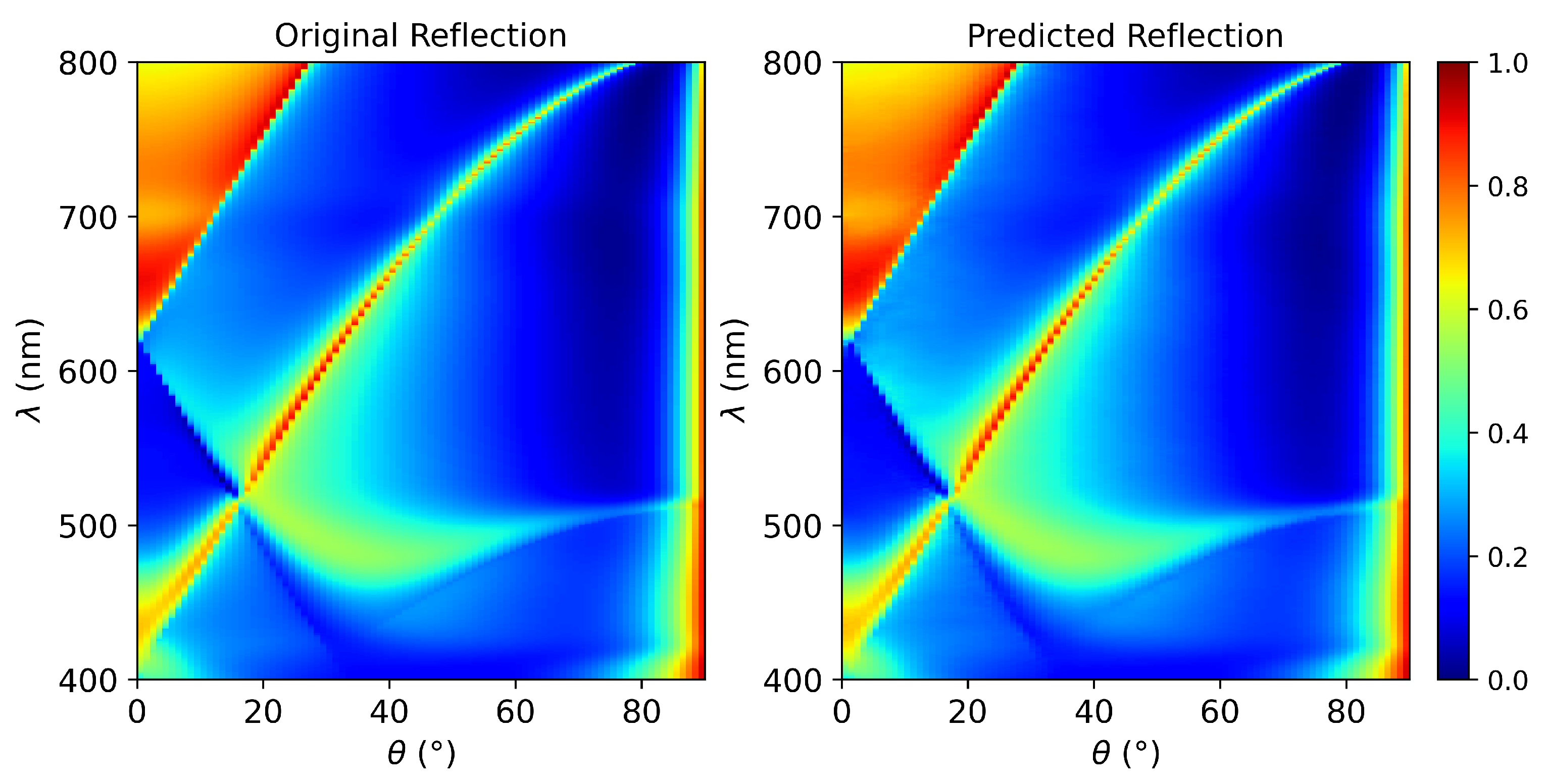
After training the AE, we trained a forward model that maps structural parameters to the AE’s latent space. The predicted latent vectors are then passed through the decoder part of the pre-trained AE to reconstruct the corresponding reflection spectra. Figure 4 illustrates this sequence of predictions by the forward model and AE for a test dataset and compares the reconstructed reflection spectra to the ground truth spectra. As shown, the model closely replicates the physical behavior of the system.

The predicted reflection spectra, obtained using the same sequence of models (forward model followed by the AE decoder), and the ground truth reflection spectra for the entire test dataset result in a MSE of 0.000136 and a MAE of 0.0056. Since reflection values are confined to the range [0, 1], the low MAE and MSE confirm the model’s ability to accurately reconstruct the system’s physical response.

To test the generalization of our models, we reserved 20% of the total 15,000 data as a test set, fully withheld during model development. The remaining 80% was used in a 5-fold cross-validation to evaluate the model. For each fold, we trained the model on 80% of the fold’s data and validated it on the remaining 20%.

All reported metrics written in

Table 1. MSE and MAE comparison of cVAE and Tandem network. The average values over the five models and their standard deviations are written here. All the values are calculated using the normalized test dataset.

Model	MSE	MAE
cVAE	$2.9\times {10}^{-4}\pm 3.64\times {10}^{-5}$	$0.0068\pm 5.5\times {10}^{-4}$
Tandem Network	$2.6\times {10}^{-4}\pm 3.58\times {10}^{-5}$	$0.0050\pm 1.0\times {10}^{-4}$

and

Table 2. The comparison of the coefficient of determination ($R^2$) of the cVAE and Tandem network. The average values over the five models and their standard deviations are written here. All the values are calculated using the normalized test dataset.

Model	${\mathit{R}}^2\left(\mathit{Ag}\right)$	${\mathit{R}}^2\left(\mathit{OrmoCore}\right)$	${\mathit{R}}^2\left(\mathbf{\Lambda }\right)$
cVAE	$0.998\pm 7.4\times {10}^{-4}$	$0.991\pm 1.6\times {10}^{-3}$	$0.999\pm 1.9\times {10}^{-5}$
Tandem Network	$0.999\pm 3.7\times {10}^{-5}$	$0.991\pm 1.3\times {10}^{-3}$	$0.999\pm 2.7\times {10}^{-6}$

, including MSE, MAE, the coefficient of determination ($R^2$), sensitivity, and other related measures and figures, for both the Tandem network and the cVAE, are calculated on either normalized or original scale (unnormalized) withheld test data and averaged across the five folds. This approach provides a statistically reliable assessment of the model’s generalization and reduces the risk of biased evaluation due to a single train-test split.

The MAE for each structural parameter’s prediction on values in original scale test data is separately summarized in

Table 3. The average MAE over the five models and their standard deviations on real structural values of test dataset.

Model	${\mathit{t}}_{\mathit{Ag}}$ [nm]	${\mathit{t}}_{\mathit{OrmoCore}}$ [nm]	$\mathbf{\Lambda }$ [nm]
cVAE	0.74 ± 0.170	15.20 ± 0.495	0.55 ± 0.026
Tandem Network	0.45 ± 0.018	13.32 ± 0.331	0.30 ± 0.003

for both the Tandem model and the cVAE. To probe the reason behind the differences between the MAEs across parameters, the sensitivity of the reflection spectra to each of the structural parameters is quantified via a central finite-difference Jacobian. The results show that the grating period has the strongest influence, followed by the silver thickness, while the OrmoCore thickness has only a minor effect. As it is shown in

Table 4. RMS absolute sensitivity of each structural parameter.

${\mathit{s}}_{{\mathit{t}}_{\mathit{Ag}}}^{\mathbf{abs}}$$\left[\frac{1}{\mathit{nm}}\right]$	${\mathit{s}}_{{\mathit{t}}_{\mathit{OrmoCore}}}^{\mathbf{abs}}$$\left[\frac{1}{\mathit{nm}}\right]$	${\mathit{s}}_{\mathbf{\Lambda }}^{\mathbf{abs}}$$\left[\frac{1}{\mathit{nm}}\right]$
$0.0099\pm 0.0069$	$0.00032\pm 8.226\times {10}^{-5}$	$0.0707\pm 0.0557$

, the Root Mean Square (RMS) absolute sensitivity with respect to the OrmoCore thickness is $0.00032$ nm⁻¹. In comparison, the RMS absolute sensitivity for silver thickness and grating period are about 31 and 221 times larger, respectively. This explains why the models consistently predict the period and silver thickness more accurately than the OrmoCore thickness. Step-size convergence tests confirmed that the chosen finite-difference steps yield reliable sensitivity values. Further details are provided in the Appendix B.

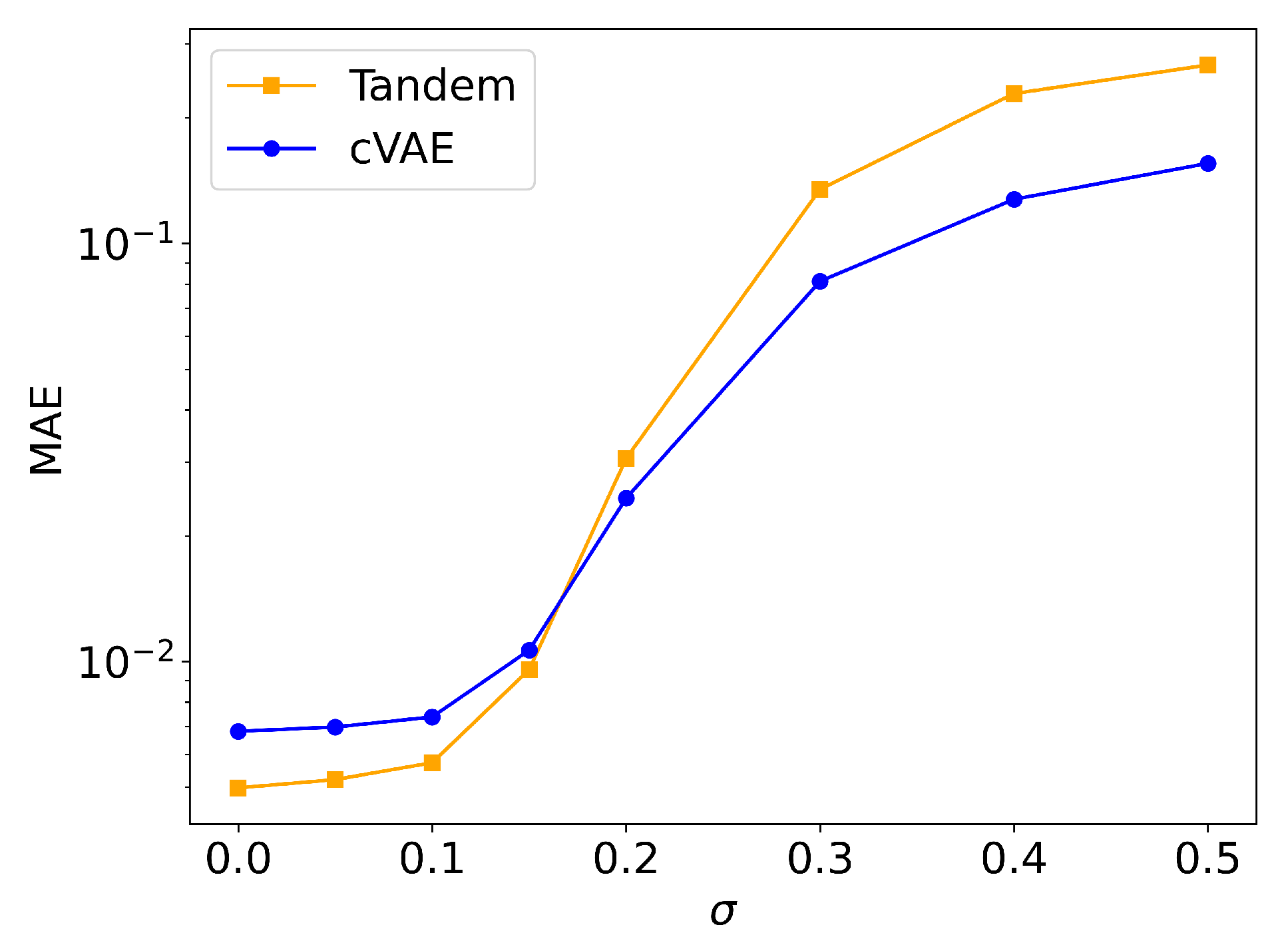
Despite training the model with noisy data, we assessed the model’s robustness by introducing noise to the reflection data and measuring how much the prediction accuracy of the structures degrades. First, the structural parameters are predicted from the noise-free test dataset, and the MAE between the prediction and the actual structural parameter is calculated. Subsequently, AGN is added to the same test dataset. The standard deviation of the noise was fixed to a constant value of $\sigma$, which was applied uniformly to all samples in the dataset. The MAE is computed again between the predicted structures from the noisy dataset and ground truth. Figure 5 illustrates this robustness analysis, showing how the MAE varies with the standard deviation, $\sigma$, of the AGN.

In addition to the normalized-scale robustness analysis, we further evaluated the effect of AGN on the absolute prediction accuracy of each structural parameter. The standard deviation of the noise was fixed to $\sigma$ for each sample in the test dataset. Figure 6 presents the MAE in real units (nm) for the silver thickness, OrmoCore thickness, and grating period, separately for both the Tandem and cVAE models.

Besides, to measure the sensitivity of the model’s predictions to small errors in the input, two predictions are obtained for each sample: one from a clean reflection spectrum and one from a noisy reflection spectrum. The standard deviation of the noise was fixed to 0.1 for each sample in the test dataset. The relative absolute difference between the two corresponding predictions is then calculated as a direct measure of sensitivity to noise, $SN$:

$$SN={\displaystyle \frac{|{\widehat{x}}_N-{\widehat{x}}_C|}{{\widehat{x}}_C}}$$

(5)

where ${\widehat{x}}_C$ and ${\widehat{x}}_N$ are the predicted denormalized, real-valued structural parameters of the clean and noisy data, respectively. The sensitivity to noise, $SN$, is computed for each sample in the test set, and the average $SN$ over all samples is calculated for each fold. Finally, the reported sensitivity to noise is the average of these values across all five folds. Sensitivity to noise is reported separately for each structural parameter, silver thickness, dielectric thickness, and period, as each may respond differently to the noise in the input reflection data. The result is shown in

Table 5. Sensitivity to noise of individual structural parameters (silver thickness, OrmoCore thickness, and grating period), averaged over five models. The details has been explain in Section 3.

Model	${\mathit{t}}_{\mathit{Ag}}$$\left[\mathit{nm}\right]$	${\mathit{t}}_{\mathit{OrmoCore}}$$\left[\mathit{nm}\right]$	$\mathbf{\Lambda }$$\left[\mathit{nm}\right]$
cVAE	$0.0048\pm 1.8\times {10}^{-4}$	$0.0253\pm 1.1\times {10}^{-3}$	$0.0004\pm 1.2\times {10}^{-5}$
Tandem Network	$0.0038\pm 6.4\times {10}^{-5}$	$0.0238\pm 1.5\times {10}^{-3}$	$0.0003\pm 4.7\times {10}^{-6}$

.

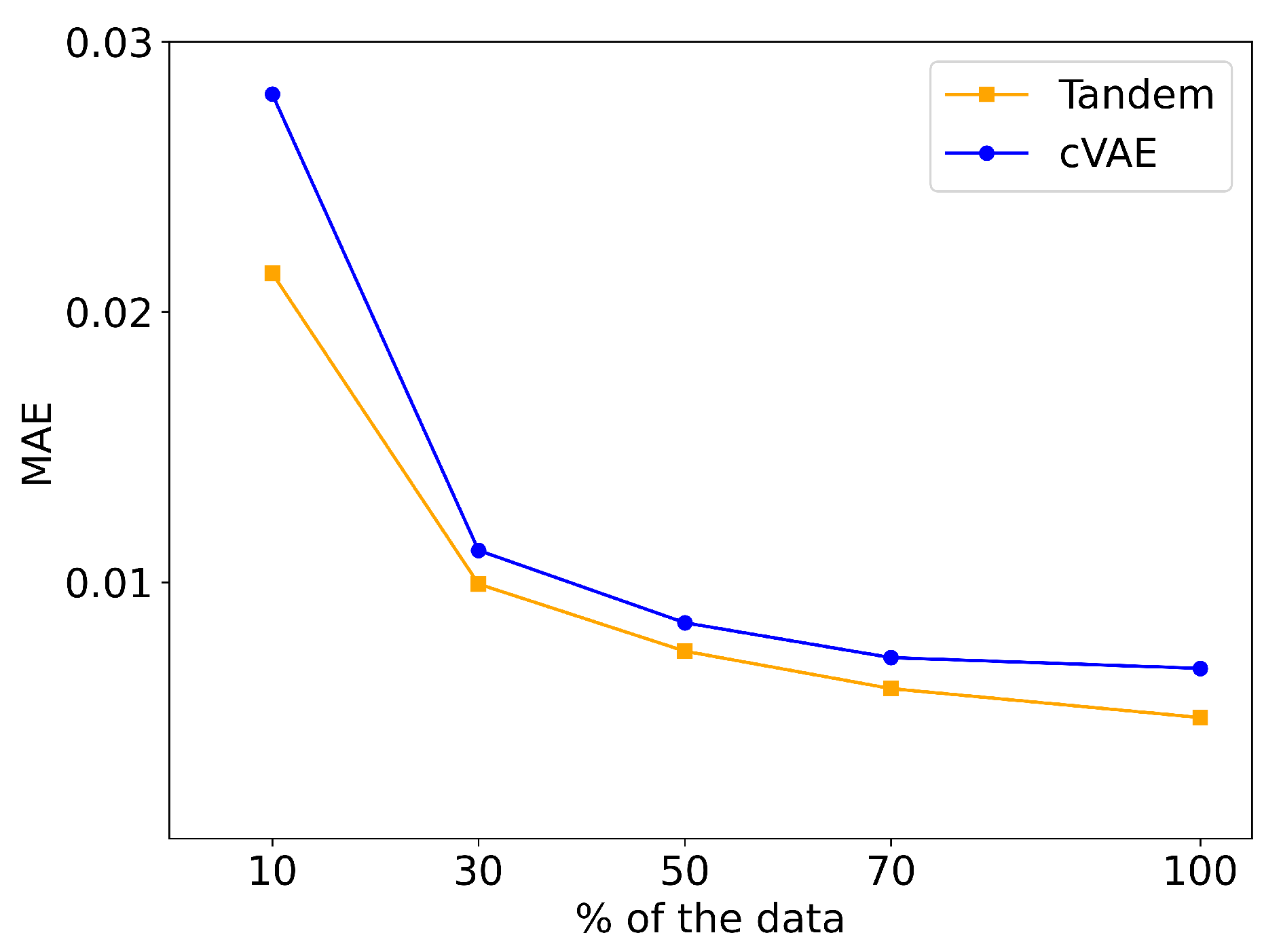
To evaluate the influence of training data availability on cVAE and Tandem models performances, we used the same architectures that were used to train each of the cVAE and Tandem but using different fractions of the full training dataset. First, the same 20% of the dataset that had been excluded during the training of the main model on the entire dataset in order to serve as an independent test set was set aside again for an unbiased evaluation. Then, 10%, 30%, 50%, 70% of the remaining data were used to train the models. For each data fraction, we performed 5-fold cross-validation. Each trained model was evaluated on the same held-out test set, and the performance was assessed using the MAE and MSE on normalized data. The reported values represent the average performance across all five folds. The results are illustrated in Figure 7.

4. Discussion

The inverse design has been extensively studied, leading to a significant corpus of research and developments. In this paper, we primarily focus on the inverse design of one-dimensional hybrid waveguide gratings composed of a silver grating on a dielectric using the reflection spectrum of the device.

Researchers who have a specific optical response in mind, which is the most suitable for their applications, can leverage our trained model to determine the corresponding structural parameters that would produce that response. This approach reduces fabrication costs and accelerates the design cycle as there is less need for trial-and-error fabrication processes.

Our model here can also assist researchers in determining the precise structural parameters of a plasmon grating structure from its measured optical response. This is particularly useful when the type of structural material is known and matches the materials used in this study, and when the grating is one-dimensional. In this case, our models can infer the structural parameters without the need for costly and time-consuming physical characterization techniques like Atomic Force Microscopy (AFM) or Scanning Electron Microscopy (SEM).

The results of this study demonstrate the effectiveness and robustness of two distinct machine learning approaches for the inverse design of hybrid waveguide gratings: the Tandem network, a discriminative model, and the cVAE, a generative model.

Our comparative analysis in Table 1 shows that the Tandem model achieves slightly better overall predictive accuracy, as evidenced by its lower MSE and MAE compared to the cVAE. Both models, however, are reliable due to the coefficient of determination ($R^2$) values in Table 2, which for both approaches are very close to unity across all structural parameters.

An evaluation of the MAE of each structural parameter in not normalized scale in Table 3 reveals that both models predict each of the structural parameters with high accuracy. Despite the larger absolute error values for the OrmoCore thickness, the relative accuracies with respect to each parameter’s design range across all three structural parameters remain within ∼1%. The sensitivity analysis, shown in Appendix B, provides a physical explanation for these differences in accuracy. Reflection spectra are significantly more sensitive to variations in grating period and silver thickness than to OrmoCore thickness. Consequently, these parameters are predicted with higher accuracy. Within the considered $(\lambda ,\theta )$ window under TM polarization, the period $\mathrm{\Lambda }$ primarily governs the resonance positions, while the silver thickness $t_{Ag}$ affects resonance coupling and damping. In contrast, the OrmoCore thickness $t_{OrmoCore}$ mainly modifies effective indices and guided-mode dispersion, which lead to comparatively weaker variations in the reflectance. This sensitivity-driven accuracy is particularly relevant for applications such as optical sensing, where resonance positions must be predicted precisely. Since the grating period dominantly governs resonance positions, its higher sensitivity enabled the AI models to predict it most accurately. From a fabrication perspective, this implies that parameters with higher spectral sensitivity must be controlled with greater precision, as even small deviations can strongly alter the reflection response. In addition, the MAE for the OrmoCore thickness is comparable to typical fabrication error encountered for instance, in spin-coating processes, particularly for thicker OrmoCore layers. Thus, the model’s prediction error for the OrmoCore thickness remains within practical fabrication tolerance.

The robustness evaluation of the models highlighted some differences between these models. Figure 5 shows how the MAE changes as a function of $\sigma$ for both the cVAE and the Tandem model. As illustrated in the plot, for low noise levels ($\sigma \le 0.15$), both models do not show significant degradation in prediction accuracy, with the Tandem model showing slightly lower MAE. At higher noise levels ($\sigma >0.2$), however, the cVAE demonstrates greater robustness to noise compared to the Tandem model.

The parameter-wise robustness analysis, shown in Figure 6, provides additional insights into the practical reliability of the models. As shown in Figure 6, the MAE of all structural parameters increases gradually with $\sigma$, indicating the sensitivity of the models to the input noise. In Figure 6a,c, both Tandem and cVAE models maintain low mean absolute errors for silver thickness and grating period at low to moderate $\sigma$. Even under strong noise levels (up to $\sigma \sim 0.2$), the MAE for silver thickness and period remains below 3 nm. As can be seen in Figure 6a,c, at $\sigma =0.3$, the MAE of the cVAE model outperforms the Tandem model, achieving errors of only 5.6 nm for the silver thickness and 5.5 nm for the grating period. Figure 6b demonstrates that the dominant error source in both models is the OrmoCore thickness, which can be attributed to the intrinsically lower sensitivity of the reflection response to changes in this parameter. Up to $\sigma \sim 0.1$ the MAE increases by only about 3 nm, from approximately 13–15 nm to 16–17 nm for Tandem and cVAE models, respectively; however, beyond this point, the error rises rapidly. A crossover in performance between the two models can also be seen. The Tandem network is preferable in scenarios with low to moderate noise, while the cVAE provides superior stability under high noise conditions, where measurement data may be significantly degraded and noisy.

We also quantified their sensitivity to noise using relative absolute differences between the predictions on clean and noisy reflection spectra under low-noise regime of $\sigma =0.1$. Based on the results shown in Table 5, the average SN values for all three structural parameters in the cVAE are higher than the corresponding values obtained from the Tandem network. It demonstrates that the Tandem network offers optimal precision for low-noise data and cVAE is more responsive to small perturbations.

To assess the performance of our cVAE and Tandem networks in the event of varying data availability, Figure 7 shows how the MAE and MSE decreases as the fraction of training data increases. Errors decrease monotonically with more data, and the Tandem model consistently yields lower MAE and MSE than the cVAE across all fractions. The performance gap is most pronounced at 10% of the data and gradually narrows at higher fractions. Beyond 70% of the training data, both models approach a saturation point, indicating that further increases in dataset size provide only marginal accuracy improvements.

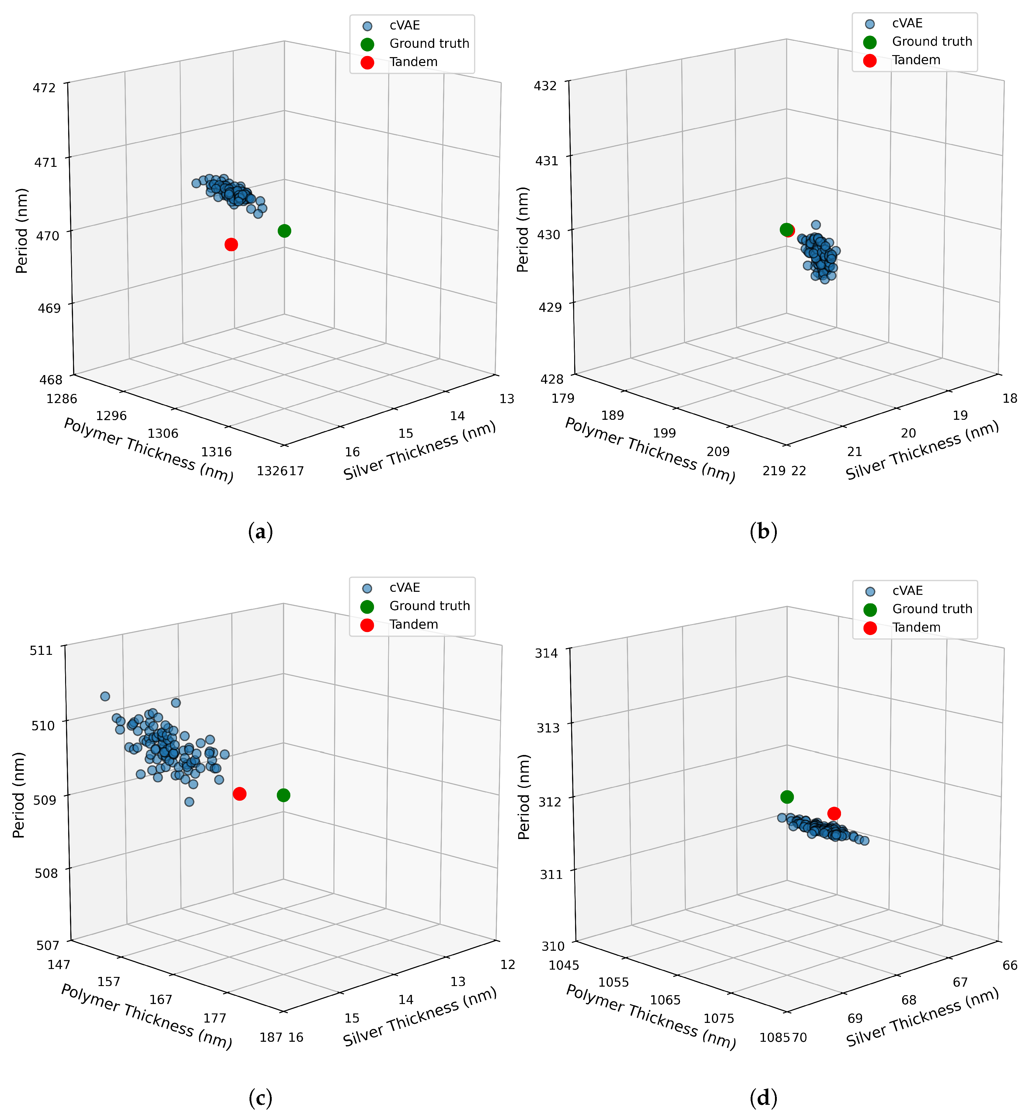
In general, each method tackles the inverse design problem differently. An inspection of Figure 8 reveals each model’s capacity to tackle the one-to-many nature of the inverse problem. Each sub-panel illustrates 100 structural predictions from the cVAE model for a single target reflection spectrum, as well as Tandem model’s prediction and the ground truth. The Tandem network provides a single, deterministic solution, which is desirable when an unambiguous, reproducible design is required. In contrast, the cVAE generates multiple valid design candidates, introducing limited diversity into the predictions. As can be seen the predictions from cVAE model yields a distribution of solutions that cluster closely around the ground truth. This indicates that the cVAE reproduces the most probable structural configurations as it captures the natural ambiguity in the inverse mapping owing to the ill-posed problem. However, this diversity remains relatively narrow due to the single-modal Gaussian assumption of the standard cVAE. Nevertheless, both model achieves high accuracy and effectively addresses the ill-posed nature of the inverse design task.

During training we added additive Gaussian white noise to the reflection spectra. AGN was used to emulate random experimental errors. Real measurements include colored noises as well. Colored noise refers to a type of stochastic noise characterized by its power spectrum that exhibits correlations across neighbouring data points, unlike white noise, which is entirely uncorrelated. Applying colored noise to reflection spectra models systematic variations such as source drifts or environmental fluctuations. Although we did not use colored noise during training, we evaluated both models under colored noises. Further information for definitions, parameters and evaluation results are provided in Supplementary Information.

In future work, we aim to explore the application of Physics-Informed Neural networks (PINNs) [49] to incorporate physical constraints directly into the learning process. This approach can improve model performances particularly for complex optical systems with less available data. Furthermore, expanding these methods to more complex structures or multi-dimensional gratings could further enhance their practical utility and scope.

5. Conclusions

In conclusion, this study presents a robust and efficient inverse design strategy for 1D hybrid waveguide gratings using machine learning models trained on reflection spectra. Both the deterministic Tandem network and the generative cVAE demonstrated high accuracy in predicting structural parameters, meeting strict design requirements for silver and dielectric thicknesses, and grating period. Notably, even under measurement conditions with substantial noise, the cVAE maintained low and reliable MAE values for silver thickness and grating period, underscoring its suitability for experimental data where noise levels may be significant.

Overall, this work highlights the potential of data-driven approaches to accelerate the design cycle, reduce fabrication costs, and eliminate the need for extensive spatial measurements, paving the way for practical applications in photonics, sensing, and integrated optical devices. Beyond hybrid gratings, the same framework can be applied to other nanophotonic structures, facilitating access to design spaces that are difficult to probe through traditional simulation approaches. Looking ahead, integrating physics-informed neural networks (PINNs) or hybrid simulation–ML workflows may further boost accuracy while reducing data requirements, strengthening the role of machine learning as a core tool for photonic inverse design.

References

1. Magnusson, R.; Wang, S.S. New principle for optical filters. Appl. Phys. Lett. 1992, 61, 1022–1024. [Google Scholar] [CrossRef]
2. Wang, J.J.; Chen, L.; Kwan, S.; Liu, F.; Deng, X. Resonant grating filters as refractive index sensors for chemical and biological detections. J. Vac. Sci. Technol. B Microelectron. Nanometer Struct. 2005, 23, 3006–3010. [Google Scholar] [CrossRef]
3. Cunningham, B.; Lin, B.; Qiu, J.; Li, P.; Pepper, J.; Hugh, B. A plastic colorimetric resonant optical biosensor for multiparallel detection of label-free biochemical interactions. Sens. Actuators B Chem. 2002, 85, 219–226. [Google Scholar] [CrossRef]
4. Magnusson, R.; Lee, K.J.; Hemmati, H.; Ko, Y.H.; Wenner, B.R.; Allen, J.W.; Allen, M.S.; Gimlin, S.; Weidanz, D.W. The guided-mode resonance biosensor: Principles, technology, and implementation. In Proceedings of the Frontiers in Biological Detection: From Nanosensors to Systems X, San Francisco, CA, USA, 27 January–1 February 2018; Danielli, A., Miller, B.L., Weiss, S.M., Eds.; Society of Photo-Optical Instrumentation Engineers (SPIE) Conference Series. SPIE: Bellingham, WA, USA, 2018; Volume 10510, p. 105100G. [Google Scholar] [CrossRef]
5. Yang, N.Z.; Hsiung, C.T.; Huang, C.S. Biosensor based on two-dimensional gradient guided-mode resonance filter. Opt. Express 2021, 29, 1320. [Google Scholar] [CrossRef]
6. Chen, W.; Long, K.D.; Lu, M.; Chaudhery, V.; Yu, H.; Choi, J.S.; Polans, J.; Zhuo, Y.; Harley, B.A.C.; Cunningham, B.T. Photonic crystal enhanced microscopy for imaging of live cell adhesion. Analyst 2013, 138, 5886–5894. [Google Scholar] [CrossRef] [PubMed]
7. Chen, W.; Long, K.D.; Yu, H.; Tan, Y.; Choi, J.S.; Harley, B.A.; Cunningham, B.T. Enhanced live cell imaging via photonic crystal enhanced fluorescence microscopy. Analyst 2014, 139, 5954–5963. [Google Scholar] [CrossRef] [PubMed]
8. Babu, S.; Lee, J.B. Axially-Anisotropic Hierarchical Grating 2D Guided-Mode Resonance Strain-Sensor. Sensors 2019, 19, 5223. [Google Scholar] [CrossRef]
9. Mattelin, M.A.; Missinne, J.; De Coensel, B.; Van Steenberge, G. Imprinted Polymer-Based Guided Mode Resonance Grating Strain Sensors. Sensors 2020, 20, 3221. [Google Scholar] [CrossRef]
10. Wang, S.S.; Magnusson, R. Theory and applications of guided-mode resonance filters. Appl. Opt. 1993, 32, 2606–2613. [Google Scholar] [CrossRef]
11. Tibuleac, S.; Magnusson, R. Reflection and transmission guided-mode resonance filters. J. Opt. Soc. Am. A 1997, 14, 1617–1626. [Google Scholar] [CrossRef]
12. Li, C.; Zhang, K.; Zhang, Y.; Cheng, Y.; Kong, W. Large-range wavelength tunable guided-mode resonance filter based on dielectric grating. Opt. Commun. 2019, 437, 271–275. [Google Scholar] [CrossRef]
13. Gu, T.; Qian, L.; Wang, K. Flat-top filter using slanted guided-mode resonance gratings with bound states in the continuum. Opt. Commun. 2022, 521, 128569. [Google Scholar] [CrossRef]
14. Dobbs, D.W.; Cunningham, B.T. Optically tunable guided-mode resonance filter. Appl. Opt. 2006, 45, 7286–7293. [Google Scholar] [CrossRef] [PubMed]
15. Liu, W.; Chen, H.; Lai, Z. Guided-mode resonance filter with high-index substrate. Opt. Lett. 2012, 37, 4648–4650. [Google Scholar] [CrossRef] [PubMed]
16. Ren, Z.; Sun, Y.; Hu, J.; Zhang, S.; Lin, Z.; Zhi, X. Electro-optic filter based on guided-mode resonance for optical communication. Electron. Lett. 2018, 54, 1340–1342. [Google Scholar] [CrossRef]
17. Snyder, A.; Love, J. Optical Waveguide Theory; Science Paperbacks; Springer: New York, NY, USA, 1983. [Google Scholar]
18. Motokura, K.; Fujii, M.; Nesterenko, D.V.; Sekkat, Z.; Hayashi, S. Coupling of Planar Waveguide Modes in All-Dielectric Multilayer Structures: Monitoring the Dependence of Local Electric Fields on the Coupling Strength. Phys. Rev. Appl. 2021, 16, 064065. [Google Scholar] [CrossRef]
19. Michelotti, F. Bloch surface waves on dielectric one-dimensional photonic crystals: Fundamental properties and applications [Invited]. Opt. Mater. Express 2025, 15, 2839–2905. [Google Scholar] [CrossRef]
20. Maier, S. Plasmonics: Fundamentals and Applications; Springer: New York, NY, USA, 2007. [Google Scholar]
21. Buchmüller, M.; Shutsko, I.; Schumacher, S.O.; Görrn, P. Harnessing Short-Range Surface Plasmons in Planar Silver Films via Disorder-Engineered Metasurfaces. ACS Appl. Opt. Mater. 2023, 1, 1777–1782. [Google Scholar] [CrossRef]
22. Oulton, R.F.; Sorger, V.J.; Genov, D.A.; Pile, D.F.P.; Zhang, X. A hybrid plasmonic waveguide for subwavelength confinement and long-range propagation. Nat. Photonics 2008, 2, 496–500. [Google Scholar] [CrossRef]
23. Meudt, M.; Bogiadzi, C.; Wrobel, K.; Görrn, P. Hybrid Photonic–Plasmonic Bound States in Continuum for Enhanced Light Manipulation. Adv. Opt. Mater. 2020, 8, 2000898. [Google Scholar] [CrossRef]
24. Johnson, P.B.; Christy, R.W. Optical Constants of the Noble Metals. Phys. Rev. B 1972, 6, 4370–4379. [Google Scholar] [CrossRef]
25. Henkel, A.; Schumacher, S.O.; Meudt, M.; Knoth, C.; Buchmüller, M.; Görrn, P. High-Contrast Switching of Light Enabled by Zero Diffraction. Adv. Photonics Res. 2023, 4, 2300230. [Google Scholar] [CrossRef]
26. Henkel, A.; Knoth, C.; Buchmüller, M.; Görrn, P. Electric Control of the In-Plane Deflection of Laser Beam Pairs within a Photonic Slab Waveguide. Optics 2024, 5, 342–352. [Google Scholar] [CrossRef]
27. So, S.; Badloe, T.; Noh, J.; Bravo-Abad, J.; Rho, J. Deep learning enabled inverse design in nanophotonics. Nanophotonics 2020, 9, 1041–1057. [Google Scholar] [CrossRef]
28. Ma, T.; Tobah, M.; Wang, H.; Guo, L.J. Benchmarking deep learning-based models on nanophotonic inverse design problems. Opto-Electron. Sci. 2022, 1, 210012-1–210012-15. [Google Scholar] [CrossRef]
29. Wiecha, P.R.; Arbouet, A.; Girard, C.; Muskens, O.L. Deep learning in nano-photonics: Inverse design and beyond. Photon. Res. 2021, 9, B182–B200. [Google Scholar] [CrossRef]
30. Deng, R.; Liu, W.; Shi, L. Inverse design in photonic crystals. Nanophotonics 2024, 13, 1219–1237. [Google Scholar] [CrossRef] [PubMed]
31. Ha, C.S.; Yao, D.; Xu, Z.; Liu, C.; Liu, H.; Elkins, D.; Kile, M.; Deshpande, V.; Kong, Z.; Bauchy, M.; et al. Rapid inverse design of metamaterials based on prescribed mechanical behavior through machine learning. Nat. Commun. 2023, 14, 5765. [Google Scholar] [CrossRef]
32. Pal, A.; Ghosh, A.; Zhang, S.; Bi, T.; Del’Haye, P. Machine learning assisted inverse design of microresonators. Opt. Express 2023, 31, 8020–8028. [Google Scholar] [CrossRef] [PubMed]
33. Liu, G.X.; Liu, J.F.; Zhou, W.J.; Li, L.Y.; You, C.L.; Qiu, C.W.; Wu, L. Inverse design in quantum nanophotonics: Combining local-density-of-states and deep learning. Nanophotonics 2023, 12, 1943–1955. [Google Scholar] [CrossRef] [PubMed]
34. Kabir, H.; Wang, Y.; Yu, M.; Zhang, Q.J. Neural Network Inverse Modeling and Applications to Microwave Filter Design. IEEE Trans. Microw. Theory Tech. 2008, 56, 867–879. [Google Scholar] [CrossRef]
35. Liu, D.; Tan, Y.; Khoram, E.; Yu, Z. Training Deep Neural Networks for the Inverse Design of Nanophotonic Structures. ACS Photonics 2018, 5, 1365–1369. [Google Scholar] [CrossRef]
36. Malkiel, I.; Mrejen, M.; Nagler, A.; Arieli, U.; Wolf, L.; Suchowski, H. Plasmonic nanostructure design and characterization via Deep Learning. Light. Sci. Appl. 2018, 7, 60. [Google Scholar] [CrossRef]
37. Wu, S.; Yamada, H.; Hayashi, Y.; Zamengo, M.; Yoshida, R. Potentials and challenges of polymer informatics: Exploiting machine learning for polymer design. arXiv 2020, arXiv:2010.07683. [Google Scholar] [CrossRef]
38. Xu, X.; Wei, Q.; Li, H.; Wang, Y.; Chen, Y.; Jiang, Y. Recognition of polymer configurations by unsupervised learning. Phys. Rev. E 2019, 99, 043307. [Google Scholar] [CrossRef]
39. Sohn, K.; Lee, H.; Yan, X. Learning Structured Output Representation using Deep Conditional Generative Models. In Proceedings of the Advances in Neural Information Processing Systems, Montreal, QC, Canada, 7–12 December 2015; Cortes, C., Lawrence, N., Lee, D., Sugiyama, M., Garnett, R., Eds.; Curran Associates, Inc.: New York, NY, USA, 2015; Volume 28. [Google Scholar]
40. Rahman, T.; Tahmid, A.; Arman, S.E.; Ahmed, T.; Rakhy, Z.T.; Das, H.; Rahman, M.; Azad, A.K.; Wahadoszamen, M.; Habib, A. Leveraging generative neural networks for accurate, diverse, and robust nanoparticle design. Nanoscale Adv. 2024, 7, 634–642. [Google Scholar] [CrossRef]
41. Mirza, M.; Osindero, S. Conditional generative adversarial nets. arXiv 2014, arXiv:1411.1784. [Google Scholar] [CrossRef]
42. Moharam, M.G.; Grann, E.B.; Pommet, D.A.; Gaylord, T.K. Formulation for stable and efficient implementation of the rigorous coupled-wave analysis of binary gratings. J. Opt. Soc. Am. A 1995, 12, 1068–1076. [Google Scholar] [CrossRef]
43. Tamir, T.; Peng, S.T. Analysis and design of grating couplers. Appl. Phys. 1977, 14, 235–254. [Google Scholar] [CrossRef]
44. Palik, E.D. Handbook of Optical Constants of Solids; Academic Press: Cambridge, MA, USA, 1998; Volume 3. [Google Scholar]
45. Polywka, A.; Tückmantel, C.; Görrn, P. Light controlled assembly of silver nanoparticles. Sci. Rep. 2017, 7, 45144. [Google Scholar] [CrossRef]
46. Polywka, A.; Vereshchaeva, A.; Riedl, T.; Görrn, P. Manipulating the Morphology of Silver Nanoparticles with Local Plasmon Mediated Control. Part. Part. Syst. Charact. 2013, 31, 342–348. [Google Scholar] [CrossRef]
47. Hinton, G.E.; Salakhutdinov, R.R. Reducing the dimensionality of data with neural networks. Science 2006, 313, 504–507. [Google Scholar] [CrossRef]
48. Vincent, P.; Larochelle, H.; Bengio, Y.; Manzagol, P.A. Extracting and composing robust features with denoising autoencoders. In Proceedings of the 25th International Conference on Machine Learning, Helsinki, Finland, 5–9 July 2008; pp. 1096–1103. [Google Scholar]
49. Raissi, M.; Perdikaris, P.; Karniadakis, G. Physics-informed neural networks: A deep learning framework for solving forward and inverse problems involving nonlinear partial differential equations. J. Comput. Phys. 2019, 378, 686–707. [Google Scholar] [CrossRef]
50. Jakob, T.; Polywka, A.; Stegers, L.; Akdeniz, E.; Kropp, S.; Frorath, M.; Schneider, T.; Trost, S.; Riedl, T.; Görrn, P. Transfer printing of electrodes for organic devices: Nanoscale versus macroscale continuity. Appl. Phys. A 2015, 120, 503–508. [Google Scholar] [CrossRef]
51. Akiba, T.; Sano, S.; Yanase, T.; Ohta, T.; Koyama, M. Optuna: A Next-generation Hyperparameter Optimization Framework. In Proceedings of the 25th ACM SIGKDD International Conference on Knowledge Discovery & Data Mining, Anchorage, AK, USA, 4–8 August 2019; KDD ‘19. pp. 2623–2631. [Google Scholar] [CrossRef]
52. Kingma, D.P.; Ba, J. Adam: A Method for Stochastic Optimization. arXiv 2014, arXiv:1412.6980. [Google Scholar] [CrossRef]
53. Loshchilov, I.; Hutter, F. Decoupled Weight Decay Regularization. arXiv 2017, arXiv:1711.05101. [Google Scholar] [CrossRef]
54. Loshchilov, I.; Hutter, F. SGDR: Stochastic Gradient Descent with Warm Restarts. arXiv 2017, arXiv:1608.03983. [Google Scholar] [CrossRef]
55. Srivastava, N.; Hinton, G.; Krizhevsky, A.; Sutskever, I.; Salakhutdinov, R. Dropout: A Simple Way to Prevent Neural Networks from Overfitting. J. Mach. Learn. Res. 2014, 15, 1929–1958. [Google Scholar]
56. Kingma, D.P.; Welling, M. Auto-Encoding Variational Bayes. arXiv 2013, arXiv:1312.6114. [Google Scholar] [CrossRef]
57. Prechelt, L. Early Stopping—But When? In Neural Networks: Tricks of the Trade, 2nd ed.; Montavon, G., Orr, G.B., Müller, K.R., Eds.; Springer: Berlin/Heidelberg, Germany, 2012; pp. 53–67. [Google Scholar] [CrossRef]
58. Gill, P.E.; Murray, W.; Saunders, M.A.; Wright, M.H. Computing Finite-Difference Approximations to Derivatives for Numerical Optimization; Technical Report SOL 80-6; Systems Optimization Laboratory, Department of Operations Research, Stanford University: Stanford, CA, USA, 1980. [Google Scholar]
59. Iott, J.; Haftka, R.T.; Adelman, H.M. Selecting Step Sizes in Sensitivity Analysis by Finite Differences; Technical Report NASA-TM-86382; NASA Langley Research Center: Hampton, VA, Australia, 1985; NASA Technical Memorandum 86382. [Google Scholar]
Figure 1. (a) A schematic depiction of the periodic 1D hybrid waveguide gratings. The waveguide consists of a silver (Ag) grating with a filling factor of 0.5 on top of an OrmoCore dielectric layer, supported by a glass substrate. The key geometrical parameters are the silver thickness, t A g , dielectric thickness, t O r m o C o r e , and grating period, Λ . (b) The zero-order TM reflection for different incident angles, θ , and wavelengths, λ , of the incident light.
Optics 06 00061 g001
Figure 3. Autoencoder reconstruction of the reflection spectra. The first row shows the clean reflection spectra (left) and its AE-reconstructed counterparts (right). The second row presents the same spectra after adding noise (left) and the corresponding reconstructions from the AE (right).
Optics 06 00061 g003
Figure 4. Visual comparison between the actual reflection spectrum (left), obtained through RCWA simulations, and the predicted spectrum (right) generated by the trained forward model followed by the AE decoder. The structural parameters used were not part of the training set, demonstrating the model’s ability to generalize and accurately approximate the reflection behavior for unseen designs.
Optics 06 00061 g004
Figure 5. Robustness evaluation of the Tandem and cVAE model against additive Gaussian noise in the reflection data. The plot shows the MAE, of the normalized predicted structural parameters on test dataset as a function of the noise standard deviation, σ . As σ increases, both error metrics rise, indicating the model’s sensitivity to input noise. The relatively gradual degradation demonstrates the model’s robustness within a reasonable noise range of σ less than 0.15.
Optics 06 00061 g005
Figure 6. Robustness evaluation of the Tandem and cVAE models against additive Gaussian noise in the reflection data for each structural parameter. The plots show the MAE of the denormalized predicted values of (a) silver thickness ( t A g ), (b) OrmoCore thickness ( t O r m o C o r e ), and (c) grating period ( Λ ) on the test dataset as a function of the noise standard deviation, σ . The error values are expressed in nanometers (nm).
Optics 06 00061 g006
Figure 7. Performance of the cVAE and Tandem models trained on increasing fractions of the training dataset (10%, 30%, 50%, 70%, 100%). Both models were evaluated on the same test set using MAE. Errors decrease monotonically with more data, and the Tandem model consistently achieves lower MAE than the cVAE across all fractions. The gap is most pronounced at 10% of the data and narrows at higher fractions. Beyond 70% of the data, both models’ MAE has reached a saturation point, indicating that additional training data do not yield significant accuracy improvements.
Optics 06 00061 g007
Figure 8. Hundred predicted structural parameters from cVAE (blue), a prediction from Tandem network (red), and ground truth (green) for four different test samples are shown in (ad). The parameters include silver thickness, polymer thickness, and period.
Optics 06 00061 g008