Rapid Discrimination of Platycodonis radix Geographical Origins Using Hyperspectral Imaging and Deep Learning

Abstract

Platycodonis radix is a commonly used traditional Chinese medicine (TCM) material. Its bioactive compounds and medicinal value are closely related to its geographical origin. The internal components of Platycodonis radix from different origins are different due to the influence of environmental factors such as soil and climate. These differences can affect the medicinal value. Therefore, accurate identification of Platycodonis radix origin is crucial for drug safety and scientific research. Traditional methods of identification of TCM materials, such as morphological identification and physicochemical analysis, cannot meet the efficiency requirements. Although emerging technologies such as computer vision and spectroscopy can achieve rapid detection, their accuracy in identifying the origin of Platycodonis radix is limited when relying solely on RGB images or spectral features. To solve this problem, we aim to develop a rapid, non-destructive, and accurate method for origin identification of Platycodonis radix using hyperspectral imaging (HSI) combined with deep learning. We captured hyperspectral images of Platycodonis radix slices in 400–1000 nm range, and proposed a deep learning classification model based on these images. Our model uses one-dimensional (1D) convolution kernels to extract spectral features and two-dimensional (2D) convolution kernels to extract spatial features, fully utilizing the hyperspectral data. The average accuracy has reached 96.2%, significantly better than that of 49.0% based on RGB images and 81.8% based on spectral features in 400–1000 nm range. Furthermore, based on hyperspectral images, our model’s accuracy is 14.6%, 8.4%, and 9.6% higher than the variants of VGG, ResNet, and GoogLeNet, respectively. These results not only demonstrate the advantages of HSI in identifying the origin of Platycodonis radix, but also demonstrate the advantages of combining 1D convolution and 2D convolution in hyperspectral image classification.

1. Introduction

Platycodonis radix is a commonly used traditional Chinese medicine (TCM) material. It is derived from the dried root of Platycodon grandiflorum (Jacq.) A. DC., typically processed into slices for medicinal use. It has the characteristics of an expectorant and soothes the throat, traditionally used to treat cough, phlegm, and chest tightness. The main active medicinal ingredients are saponins, flavonoids, and other bioactive substances [1,2,3]. The content of chemical components and the pharmacological effects of TCM materials are generally influenced by the environmental conditions of their origin. Modern research shows that Platycodonis radix from different geographical sources shows significant differences in the content and proportion of active components, which directly affect its medicinal value [4,5]. In recent years, with the growing demand for Platycodonis radix, materials from different origins have been frequently mixed and adulterated in market circulation, which has seriously affected the consistency of the medicinal quality of medicinal materials and the safety of clinical use [6]. Therefore, the development of a rapid and accurate method for identifying the origin of Platycodonis radix is in high demand and holds significant application value.

Traditional identification methods of TCM materials mainly include the classification based on morphological characteristics and the analysis techniques based on physicochemical properties. Morphological identification relies on the sensory evaluation of the appearance, color, smell, and other characteristics of medicinal materials by professionals. This method has strong subjectivity and is difficult to apply in large-scale identification of medicinal materials. By detecting the physicochemical properties of medicinal materials, the identification results are more objective and accurate. High-performance liquid chromatography (HPLC) is a widely used physical and chemical identification method, and it is also a common method in the studies on Platycodonis radix. Many spectroscopic techniques, such as Inductively Coupled Plasma Atomic Emission Spectrometry (ICP-AES) and Fourier Transform Infrared (FTIR) spectroscopy, have also been employed for the quality control of Platycodonis radix [7,8,9]. However, physicochemical analysis methods commonly suffer from disadvantages such as complex sample pretreatment and sample damage, making it difficult to meet the needs of rapid non-destructive testing. With the development of biotechnology, molecular identification technologies such as DNA barcoding and biochips have provided new solutions for the identification of TCM materials [10]. These methods can achieve highly accurate identification, but still face significant challenges in industrial rapid identification applications due to high costs and long detection cycles.

In recent years, intelligent sensing technologies represented by computer vision, electronic nose, and electronic tongue have shown significant advantages. These technologies enable the digital characterization and non-destructive detection of TCM material properties by simulating human sensory functions [11]. In particular, computer vision technology has been widely applied in TCM materials identification due to its ultra-high detection efficiency. For example, Chen et al. [12] developed an automated recognition system based on computer vision and machine learning, which achieved high-precision identification of 315 common TCM materials, with an accuracy of 99.2%. However, computer vision technology mainly relies on the morphological and texture features of TCM materials and cannot capture the internal chemical composition information. This leads to significant limitations in applications that require higher resolution, such as source recognition. In contrast, near-infrared (NIR) spectroscopy is based on the interaction between the vibration absorption of overtones and combination tones of chemical bonds (such as O-H, C-H, N-H, etc.) in molecules and the NIR photon energy, which can reflect the molecular vibration information of samples and provide an effective means for component analysis [13]. NIR spectroscopy has been widely applied in medical and agricultural fields. Addissouky et al. [14] combined NIR spectroscopy technology with machine learning to achieve rapid detection of liver fibrosis; Guo et al. [15] realized real-time monitoring of potato dry matter content by using NIR spectroscopy technology. However, due to the lack of spatial resolution, the performance is still not ideal when dealing with identification tasks that rely on spatial features [16].

Compared with computer vision and NIR spectroscopy, hyperspectral imaging (HSI) has obvious advantages. It can simultaneously collect spatial and spectral information of the target and construct a spatial spectral data cube. This cube not only contains the image information of the sample, but also records the spectral response of each pixel in the continuous spectrum. In addition, HSI technology also has the advantages of being non-contact, non-destructive, and highly efficient, making it suitable for large-scale batch detection. It has been widely used in agriculture, medical diagnostics, food quality assessment, and other fields [17,18,19]. In recent years, it has also been increasingly applied in the field of TCM materials identification, such as authenticity identification, attribute identification, component quantification, and so on [5]. Different TCM materials contain varying chemical components, resulting in distinct spectral responses, particularly in the NIR bands. HSI can more comprehensively capture these differences, which is helpful to improve classification accuracy. Wu et al. [20] successfully distinguished 11,038 chrysanthemum samples from seven varieties by using HSI technology, and the accuracy in the training set and the test set was close to 100%; Zhang et al. [21] used HSI technology to identify the growth years of Puerariae Thomsonii radix, and the accuracy of the ternary classification task was up to 90.15%. These studies proved the feasibility of HSI in the field of TCM materials identification.

The composition of Platycodonis radix is complex and closely related to its geographical origin. However, due to the uneven spectral distribution of the surface of slices, it is difficult to achieve high classification accuracy by NIR spectroscopy based solely on spectral data. At the same time, there is a lack of significant differences in the surface appearance of Platycodonis radix slices from different regions, and thus classification based solely on RGB images also fails to achieve high accuracy. To improve the accuracy of origin discrimination of Platycodonis radix slices under rapid and non-destructive conditions, we employed HSI to integrate both spatial and spectral features. In this study, we propose an intelligent geographical discrimination approach of Platycodonis radix origin based on HSI and deep learning. The hyperspectral image dataset of Platycodonis radix slices was constructed by collecting representative samples from four origins, and a deep learning algorithm combining one-dimensional (1D) convolution and two-dimensional (2D) convolution was developed to fully extract spatial and spectral features.

2. Materials and Methods

2.1. Sample Preparation

Platycodonis radix samples were collected from Anhui, Hebei, Inner Mongolia, and Zhejiang provinces in China, all of which were biennial cultivated varieties. Platycodonis radix was purified to remove impurities, washed with flowing water, and then cut into 2–4 mm standard thick slices and dried to constant weight to make Platycodonis radix herbal slices. Herbal slice is a common medicinal form of Platycodonis radix. As shown in Figure 1, slices are irregular in shape, with ring lines on the section. A total of 225 slices were randomly selected from the samples of each origin (900 slices in total for all four origins). These slices were dried, preserved, and prepared for the construction of a classification model.

2.2. HSI System

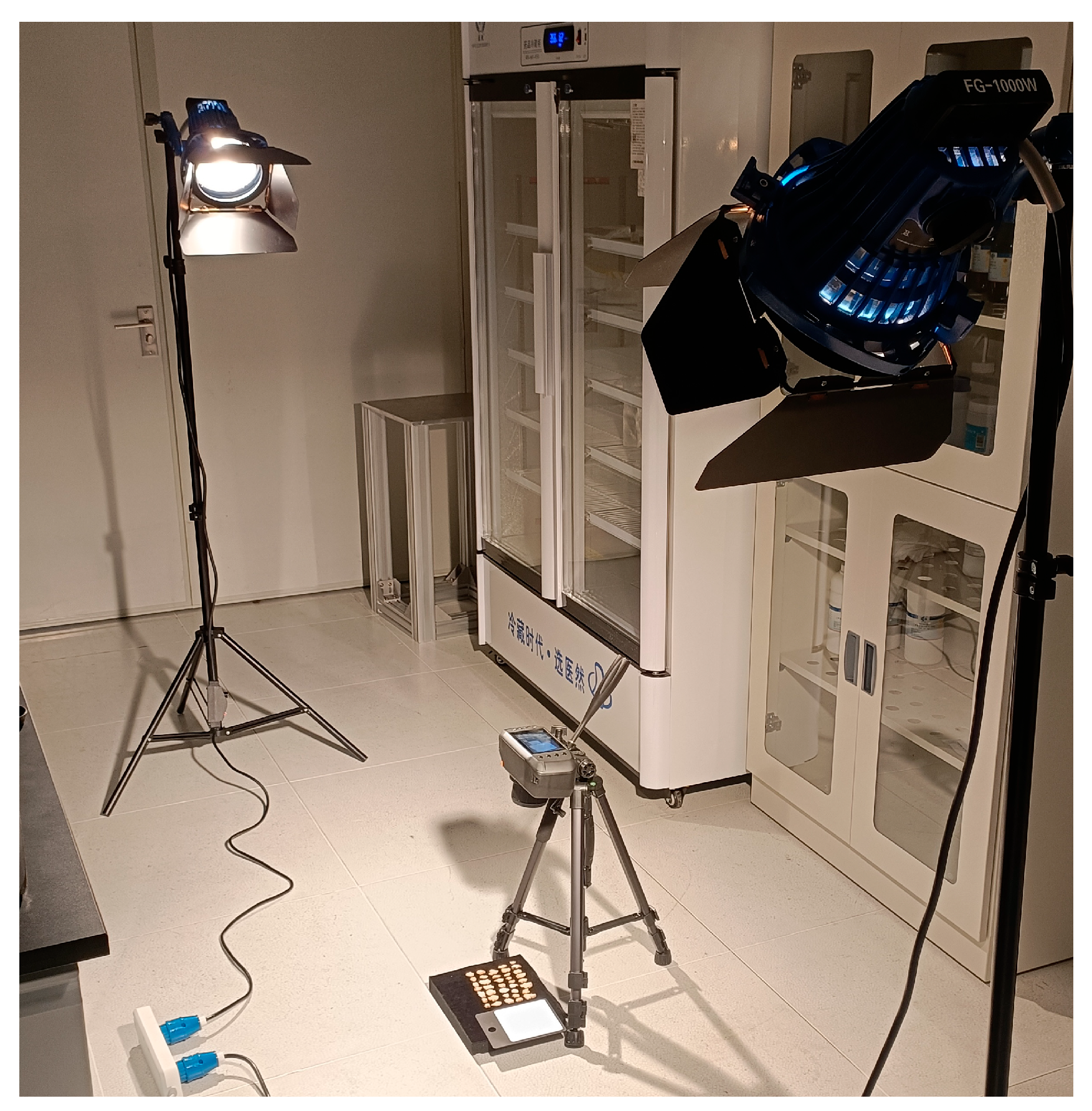
The HSI system used in this study is shown in Figure 2. The equipment used for hyperspectral image acquisition is a handheld hyperspectral camera, Specim-IQ (Specim Ltd., Oulu, Finland). The hyperspectral image acquisition is realized through internal push-broom imaging. The band of Specim-IQ covers 400–1000 nm, belonging to the visible-near-infrared (Vis-NIR) range, and the number of bands is 204. The spectral resolution is 7 nm, and the exposure time was set to 50 ms for all image acquisitions in this study.

The camera is fixed on a tripod. It adopts the vertical down imaging mode to keep the optical axis of the lens strictly vertical to the sample plane, and the working distance is fixed at 35 cm. The lighting equipment is two Bolangte FG-1000W tungsten spotlights (Hongtu Zhanfei Technology Co., Ltd., Shenzhen, China), color temperature is 3200 K. The lamp cap height is fixed at 170 cm, the transverse distance from the sample center is fixed at 150 cm, and the angle is fixed at 45° downward.

To eliminate the influence of ambient stray light, the image acquisition was carried out in a dark room, and all light sources except tungsten filament lamps were turned off. Samples were placed on the black flocking cloth background surface with very low reflectivity to reduce the light scattering effect and improve the image acquisition accuracy. Before imaging, adjust the camera’s focal length, aperture, exposure time, and other key parameters to ensure a clear image. In addition, a white board (made of high-purity polytetrafluoroethylene, with reflectivity > 99% in the visible-near-infrared band) that is compatible with the Specim IQ should be placed in the field of view when imaging, used for converting the raw data into reflectance [22]. The formula is:

$$Ref={\displaystyle \frac{Raw-Dark}{White-Dark}}$$

(1)

where $Raw$ is the spectral reflection value of the sample, $Dark$ is the spectral reflection value of the blackboard (the camera can automatically obtain it without additional imaging), and $White$ is the spectral reflection value of the white board. In order to ensure the reliability of the imaging results and avoid other interference factors, the imaging of all samples is completed in one process. One 3D data cube is obtained each time.

2.3. Dataset Construction

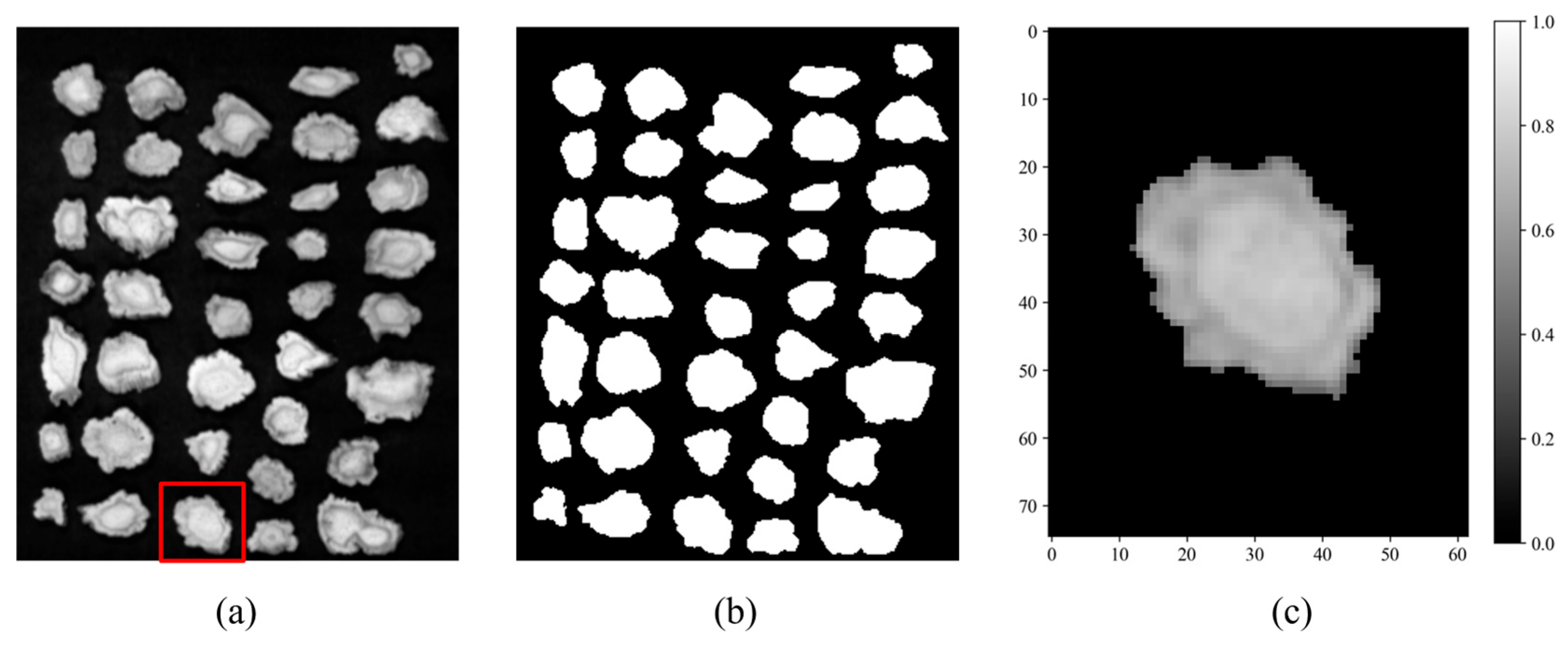
Each hyperspectral image contains a number of Platycodonis radix slices. In order to meet the needs of subsequent model training, it is necessary to segment multiple sample images into multiple independent single sample images. Firstly, as shown in Figure 3a, the original hyperspectral image containing multiple samples is summed to generate a 2D gray image; Then, as shown in Figure 3b, k-means clustering (with k = 2) is applied to the gray image, where pixels with intensity values ≥ 50 are assigned to decision 1 (Platycodonis radix label, white: 255), while pixels with values < 50 are assigned to decision 0 (black flocking cloth background label, black: 0) to obtain the binary image, which realizes the separation of Platycodonis radix and background. Next, the contour of each Platycodonis radix slice is extracted from the binary image using the cv2.findcontours() function based on the contour tracking algorithm in OpenCV, and the corresponding pixel region is extracted from the original hyperspectral image. Calculate the minimum circumscribed rectangle of each pixel region, and make them unified into patches of the same size by adding padding around all the rectangles. The height and width of the patch are the maximum values of the height and width of all the smallest circumscribed rectangles of the slice, respectively. In this study, as shown in Figure 3c, the patch size is 75 × 62. This method realizes the full automation of dataset construction and ensures that each slice can be used as an independent sample for subsequent classification tasks. Compared with the traditional method of building datasets by manually clipping regions of interest (ROI) in ENVI 5.6 software (Research Systems Inc., Boulder, CO, USA), it is not only more efficient, but also closer to the method of target extraction in actual detection, reducing uncertainty. As mentioned above, there are 225 samples of Platycodonis radix slices from each of the four origins. In each origin, we used 200 of them to train the classification model, and the remaining 25 are ready to be used as the test set to test the model’s performance, resulting in 800 training samples and 100 test samples in total. The samples used for training cover the spectral characteristics of Platycodonis radix from different origins, ensuring that the model can learn their spectral differences and accurately distinguish test samples in the subsequent classification task.

2.4. Preprocessing

In order to achieve classification tasks more successfully, we preprocessed the spectra before starting data training. First, we deleted 10 bands with low signal-to-noise ratio before and after the spectral bands, reducing the overall number of bands from 204 to 184 (which means that the size of the hyperspectral image samples input to the model is 184 bands × 75 pixels × 62 pixels). Then, we smoothed the remaining spectra using Savitzky–Golay (SG) filtering (with a polynomial order of 2 and a window length of 5 points), and finally processed the spectra with first-order derivatives to enhance the ability to distinguish spectral features [23,24]. In the image preprocessing stage, we used data augmentation methods such as horizontal and vertical flipping for the training set samples to increase randomness.

2.5. Origin Classification Network Model

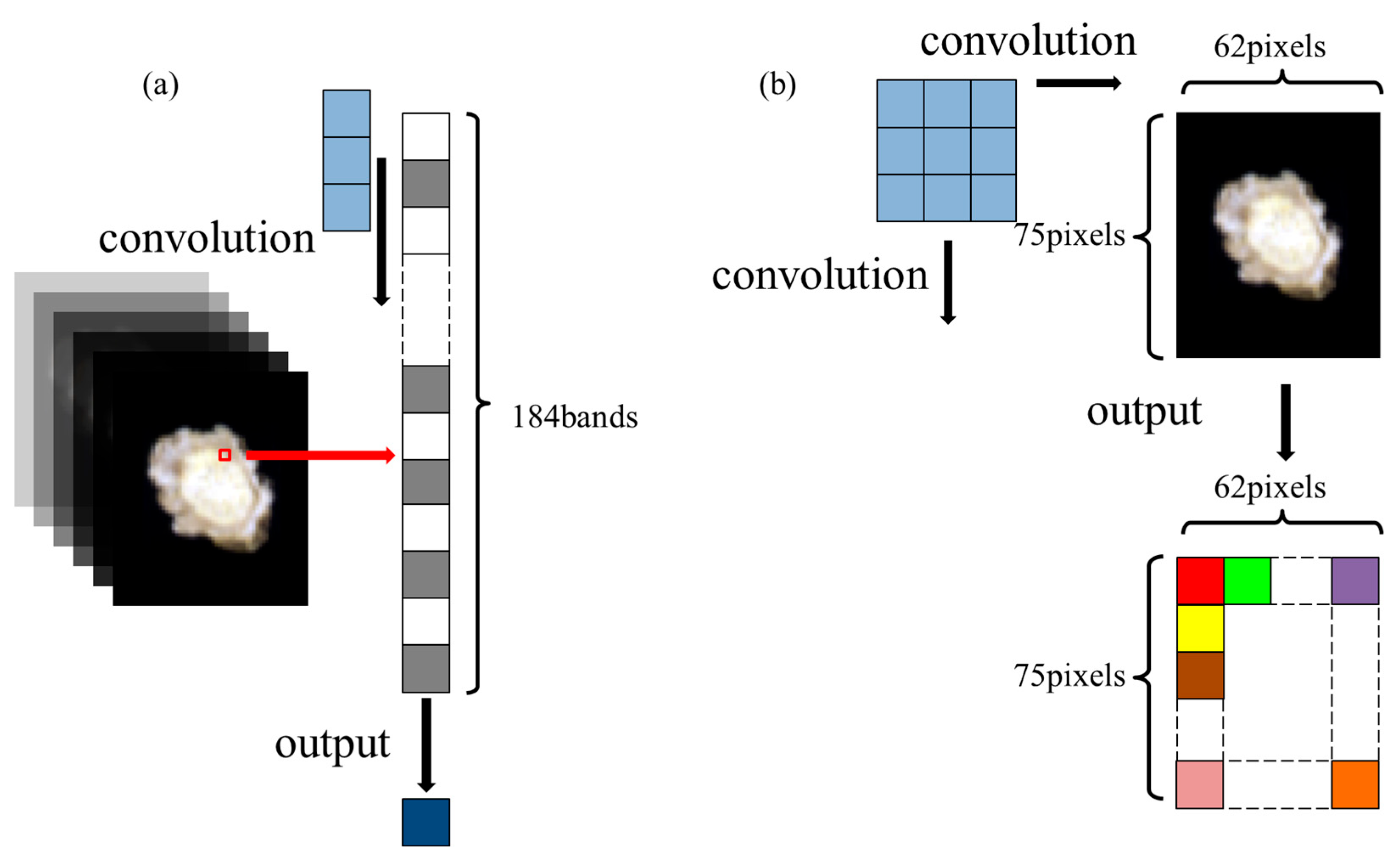
In this study, we used a hybrid convolution module for convolutional operation. Among them, the 1D convolutional kernel is responsible for extracting spectral information, and the 2D convolutional kernel is responsible for extracting spatial information. Before 1D convolution, the pixels of the image were flattened into a pixel sequence. As shown in Figure 4a, the 1D convolutional kernel slides along the band dimension of each pixel to learn the spectral features. Unlike 1D convolution, the 2D convolutional kernel slides on the 2D plane of the image along both height and width directions, which is shown in Figure 4b.

Taking the first convolution operation as an example, the 1D convolutional kernel size was set to 3 and the step size was set to 1. Before convolution we added a padding to each end of the band (the same operation is performed before each 1D convolution), and the feature output remained unchanged after convolution, still 184. Then, we reshaped the pixel sequence back to its original shape, and added a circle of padding around the 2D image as well (the same operation was performed before each 2D convolution). Finally, we performed a 2D convolution operation, the kernel is 3 × 3 in size and has a step size of 1. The size of the final output feature map remained unchanged. The entire first convolution process is shown in Figure 5.

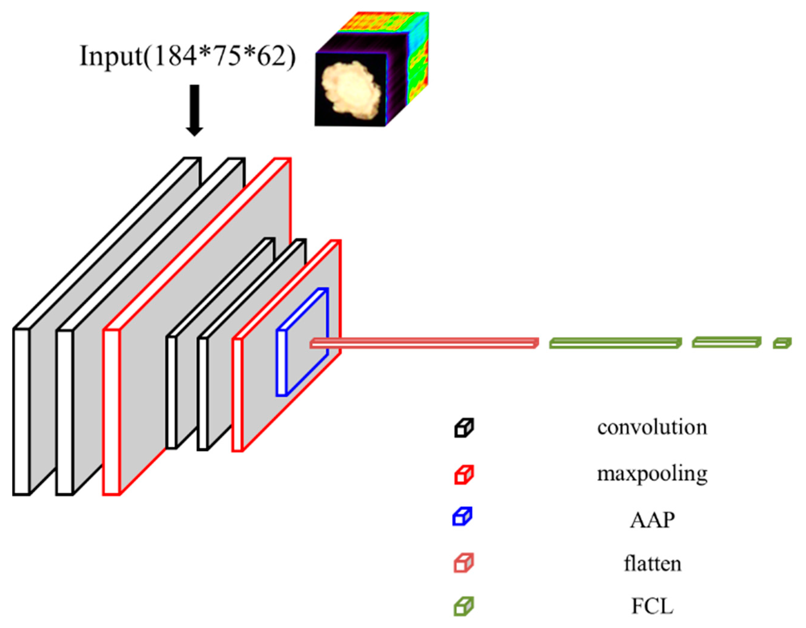
After every two convolution operations, max pooling was performed with kernel size 2 × 2 and stride 2. The kernel slides the window in the spatial dimension and takes the maximum value in the local region, thereby achieving spatial downsampling of the feature map, reducing the size of the feature map, preserving the main feature information and cutting computational costs. After processing through four convolution and two max pooling blocks, adaptive average pooling (AAP) was performed to adjust the feature map to a fixed size of 10 × 10, ready to enter the fully connected layer (FCL). FCL is an important component of classification models, whose core is to combine and map features through linear transformations and nonlinear activation functions, mapping the input features of the previous layer to the output features. Before entering the linear FCL, the data features were flattened into a sequence. After passing through three linear FCLs, the final output feature dimension is 4, corresponding to the classification labels of four origins. The complete structure is shown in Figure 6.

The classification model was implemented in Python 3.11.7 using the PyTorch 2.3.1 framework (Facebook AI Research, New York, NY, USA) within the PyCharm IDE 2024.1 (JetBrains, Prague, Czech Republic).

2.6. Training Settings

To make full use of data and improve the performance of the model, we employed K-fold cross-validation for model training and validation. We set K as 5, then samples were randomly divided into five equally sized, non-overlapping subsets. The model was trained five times. In each iteration, one of the subsets was used as the validation set, and the remaining four were used as training sets [25]. This strategy ensures that each sample is used for the validation once. In our study, each training set has 640 samples, and each validation set has 160 samples. Hyperparameter selection is also crucial for the model. Based on a series of preliminary experiments, we determined the final settings. The number of epochs was set to 1600 to ensure full convergence. The optimizer used was AdamW, which effectively controls parameter updates and prevents overfitting. The learning rate was set to $5\times {10}^{-7}$ to improve stability and avoid oscillations during training, and the weight decay was set to $1\times {10}^{-4}$ to regularize the parameters and prevent overfitting. The batch size was set to 8 to balance training stability and resource usage.

2.7. Model Performance Evaluation

Classification accuracy is the primary evaluation metric for assessing classification performance. The calculation formula of accuracy in 5-fold cross-validation is:

$$Acc={\displaystyle \frac{1}{5}}\sum _{k=1}^5\left({\displaystyle \frac{{\sum }_{i=1}^4{C}_{ii}^{\left(k\right)}}{{\sum }_{i=1}^4{\sum }_{j=1}^4{C}_{ij}^{\left(k\right)}}}\right)\times 100\mathrm{\%}$$

(2)

where $C_{ij}^{\left(k\right)}$ represents the number of samples whose true class is i but is predicted to be j in the k-th fold, and ${\sum }_{i=1}^4{\sum }_{j=1}^4{C}_{ij}^{\left(k\right)}$ represents the total number of samples across all categories; $C_{ii}^{\left(k\right)}$ indicates the number of correctly classified samples, i.e., the instances where the prediction matches the true class. Classification accuracy should be calculated not only on the test set but also on the training and validation sets, as this helps evaluate the model’s performance throughout the training process.

The loss value is used to quantify the difference between the predicted results of the model and the true labels. In each epoch, the model compares its predictions with true labels, and calculates the loss value using the loss function. The loss function used in this study is cross-entropy, which is particularly suitable for classification tasks [26]. The calculation formula is:

$$Loss=-{\displaystyle \frac{1}{N}}\sum _{n=1}^N\sum _{i=1}^K{y}_{i,n}\mathit{log}\left(p_{i,n}\right)$$

(3)

where N and K are the numbers of samples and categories, respectively. $y_{i,n}$ denotes the one-hot encoding of the true class for sample n, if sample n belongs to class i, then $y_{i,n}$ is 1, otherwise, it is 0. $p_{i,n}$ represents the predicted probability that sample n belongs to class i. The higher this probability is, the lower the loss is.

3. Results and Discussion

3.1. Spectral Analysis

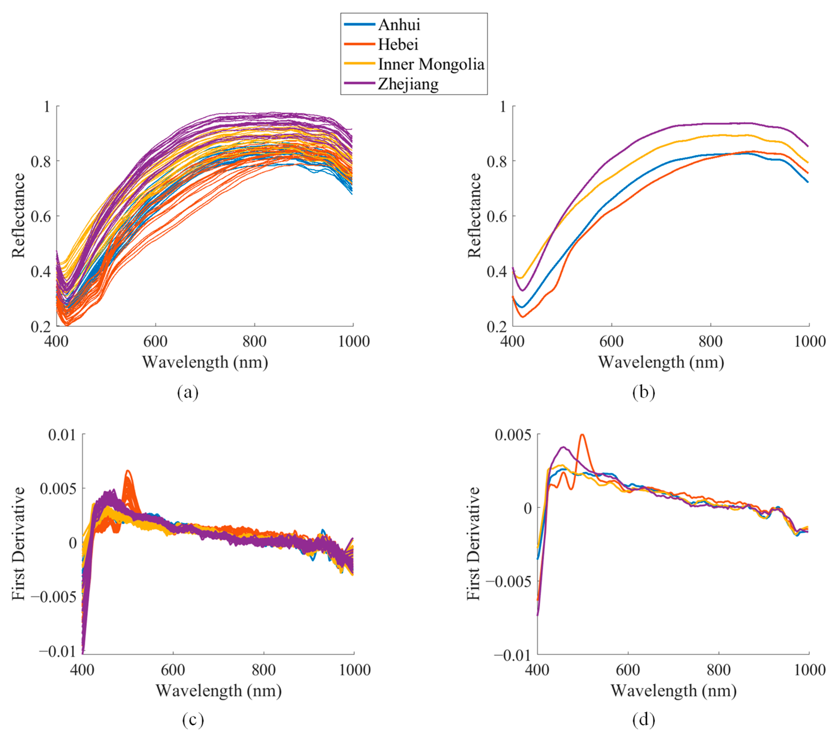
To verify the spectral differences in Platycodonis radix from different origins and confirm the feasibility of the study, we used Matlab R2023a (The Mathworks, Natick, MA, USA) to analyze the spectral data. We randomly selected 20 samples of slices from the training sets of four origins, and then took 5 × 5 pixels (25 pixels total) from the center of each sample as the region of interest (ROI). We calculated the average spectral reflectance of the 25 pixels in each ROI, obtained the average spectral curve of each sample, and then used SG filtering (polynomial order = 2, window length = 15) to smooth the data and reduce noise. The results are shown in Figure 7a. Then, the spectral curves of the 20 samples from each origin were averaged again to obtain a representative curve for each origin, as shown in Figure 7b. From Figure 7a,b, we can see the spectral variation trend of the Platycodonis radix slices. In the visible range, the reflectance initially decreases and then rises, forming an absorption peak around 420 nm, which corresponds to the strongest absorption of blue-violet light. This is one of the key reasons why Platycodonis radix slices appear yellowish-white. In the NIR range, the reflectance initially stabilizes and then exhibits a pronounced decrease around 970 nm. Figure 7a,b show that the average spectral curves from different origins have similar trends, but there are still certain differences. We applied the first derivative to the spectra in Figure 7a,b, and the results are shown in Figure 7c,d, respectively. This step removes baseline drift and highlights spectral differences more clearly.

3.2. Model Classification Performance

The input hyperspectral image is propagated forward through nonlinear transformations in each layer of the model, and the loss value is calculated. Then, the model parameters are updated based on the loss value through backpropagation. Figure 8 shows the loss curve, accuracy curve, and confusion matrix of the validation result. The loss curve (Figure 8a) shows the learning dynamics of the model during the training process. The training loss and validation loss decrease rapidly in the initial stage, and then tend to stabilize, indicating that the model fits well and avoids overfitting. Figure 8b shows the accuracy curves of the model on the training and validation sets. The training accuracy rapidly increases in the first few training epochs and eventually reaches 100%. The rate of validation accuracy increase is slower, but the overall trend is similar. The final average accuracy of validation reached 97.6%, thus verifying the reliability of the model on the validation set. The confusion matrix shown in Figure 8c can reflect the classification ability of the model in four origins. The average accuracy in the four origins of Anhui, Hebei, Inner Mongolia, and Zhejiang are 96.5%, 98.0%, 97.5%, and 98.5%, respectively. Through the results, it can be seen that the model not only achieves good fitting performance on the training set, but also has stable classification performance on the validation set, and is capable of handling the task of classifying the origin of Platycodonis radix.

3.3. Real-World Application Validation

Although the validation set has been used to evaluate the generalization ability of the model during training, the good performance on the validation set itself is the result of our continuous adjustment of the network structure and hyperparameters, which has a bias. Therefore, the actual classification performance of the model still needs to be tested. The test set is data that the model has never seen before and can provide a realistic evaluation of the model on unseen data. Therefore, it is significant to verify the accuracy of the classification model on the test set.

As mentioned earlier, 25 samples were selected from each origin as the test set, which were taken independently of the training and validation sets. They were randomly divided into 4 groups of 25 and placed randomly (but the correct origin of slice is marked at each location). During detection, patches containing Platycodonis radix slice are extracted using the same processing method as when automatically constructing the training dataset. This detection method is closer to real detection scenarios and further tests the model’s generalization ability and robustness on unseen data, enabling it to be truly applied.

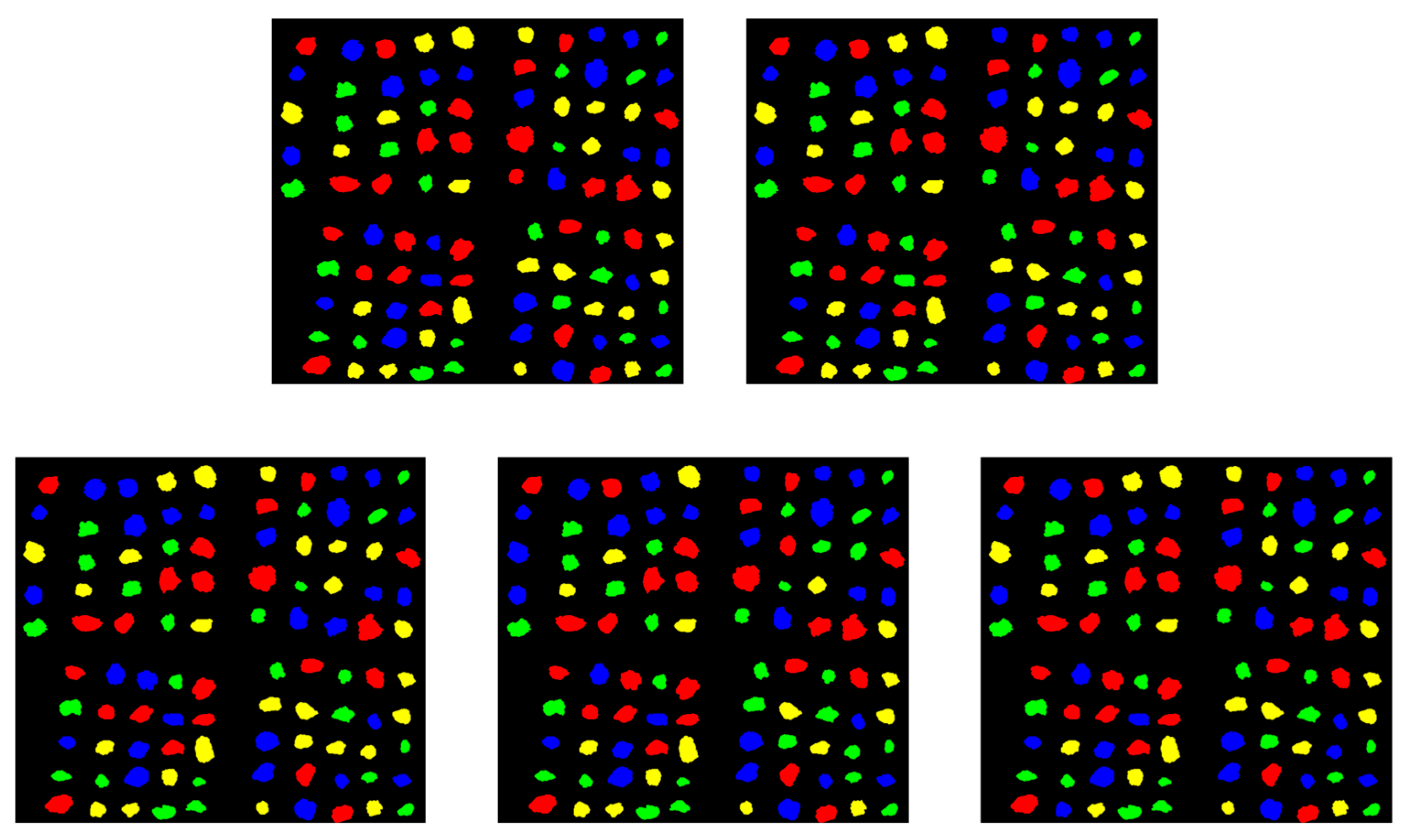
After each iteration, the model updates its weights and biases, and the best-performing model—based on validation accuracy—is saved (as a .pth file) for classifying the test set. Although performing best on the validation set does not necessarily mean performing well on the test set, this approach can still be an effective way to improve generalization ability. After processing, hyperspectral images are still detected by the model as individual samples of Platycodonis radix. The final test results of the model are displayed by assigning corresponding color masks to Platycodonis radix slices from different origins: green represents Anhui, yellow represents Hebei, blue represents Inner Mongolia, and red represents Zhejiang. The color mask results for each fold are shown in Figure 9, the accuracies are 98%, 98%, 96%, 92%, and 97%, respectively. The average accuracy is 96.2%, which is just a little lower than that of the validation set, indicating that the model does have strong generalization ability. Figure 10a shows the testing confusion matrix.

There have been many studies on identifying TCM materials using HSI method, but research on classifying the origins of Platycodonis radix has not been reported. Our study used hyperspectral imaging combined with deep learning to distinguish the origin of Platycodonis radix, which has non-destructive advantages compared to traditional methods of Platycodonis radix origin identification. In terms of model construction, our study integrates 1D convolution and 2D convolution structures, which can more fully extract spatial and spectral features from hyperspectral images. Compared with using only 2D convolution methods, it significantly improves the feature expression ability [27,28,29]. In addition, in many studies, researchers create datasets by manually cropping hyperspectral images, whereas our method can automatically create datasets based on hyperspectral images, achieving full automation from training to detection. This provides a reference solution for practical applications. However, in our study, the NIR wavelength range is relatively narrow, which limits further improvement in accuracy.

3.4. Ablation Study

To demonstrate the superiority of hyperspectral imaging, we simultaneously compared the results based on RGB image and spectral feature classification. Specim IQ can simultaneously capture the corresponding RGB images while acquiring hyperspectral images, so we also obtained the RGB images. For classification, 200 images per origin were used for training and 25 for testing. The preprocessing procedure is the same as that used for hyperspectral images. To enhance data diversity, each image in the training set is augmented using horizontal and vertical flipping. For comparative experiments, we trained, validated, and tested these RGB images using the same method and the same model architecture, but with only 2D convolutional kernels considering the differences in data characteristics. We tuned the hyperparameters multiple times, the best average classification accuracy based on RGB images is only 49.0% as shown in the confusion matrix results in Figure 10b. This result indicates that although RGB images can provide visual information, they contain limited feature information related to the origin of Platycodonis radix.

In the preprocessing of hyperspectral images, we applied contour detection and image segmentation techniques to extract the region of Platycodonis radix slice. To obtain the spectral data of Platycodonis radix, we calculated the average reflectance of all pixels in the slice region for each band and saved it as a CSV file. As before, 200 slice samples per origin were used for training, and 25 for testing. Then, we performed the same spectral preprocessing procedures as the hyperspectral images. The architecture of the classification model remains unchanged, but only 1D convolutional kernels are employed to better adapt it to the linear structure of the spectral data. We tuned the hyperparameters multiple times, and the best classification result is shown in the confusion matrix in Figure 10c, with an accuracy of 81.8%. Compared with these two methods, the accuracy of hyperspectral imaging has been improved by 47.2% and 14.4%, respectively, demonstrating its significant advantage in multi-class TCM materials classification tasks. This advantage is mainly attributed to its simultaneous fusion of spatial and spectral information, which can comprehensively characterize the morphology and internal chemical composition of TCM materials.

In Supplementary Materials, we also compared the classification results of three mainstream models, VGG, ResNet, and GoogLeNet, with accuracies of 81.6%, 87.8%, and 86.6%, respectively. In addition, we also compared the classification results after dimensionality reduction using PCA, with an accuracy of 93.2%.

4. Conclusions

In this study, we achieved non-destructive, fast, accurate, and fully automatic identification of four origins of Platycodonis radix slices using hyperspectral imaging and deep learning. Results show that the average accuracy of this method reaches 96.2%, which is significantly higher than that of RGB image-based and spectrum-based methods. In addition, we proposed a new model that integrates 1D and 2D convolution, which is capable of extracting both spectral and spatial information, and demonstrating strong recognition ability and robustness. The outcome of this study provides strong technical support for quality control, market supervision, and the traceability system of TCM materials. The technical framework proposed in this study has strong universality and can be extended to the origin tracing scenarios of other TCM materials in the future, offering more possibilities for quality assurance in related fields. In future work, we will further explore cross-temporal and cross-spatial validation, as well as the integration of multispectral or data-fusion methods, to comprehensively evaluate and enhance the robustness and generalizability of the proposed framework.

References

1. Chinese Pharmacopoeia Commission. Pharmacopoeia of the People’s Republic of China, 2020th ed.; China Medical Science Press: Beijing, China, 2020; Volume I. [Google Scholar]
2. Zhang, L.; Huang, M.; Yang, Y.; Huang, M.; Shi, J.; Zou, L.; Lu, J. Bioactive platycodins from Platycodonis radix: Phytochemistry, pharmacological activities, toxicology and pharmacokinetics. Food Chem. 2020, 327, 127029. [Google Scholar] [CrossRef]
3. Huang, W.; Lan, L.; Zhou, H.; Yuan, J.; Miao, S.; Mao, X.; Hu, Q.; Ji, S. Comprehensive profiling of Platycodonis radix in different growing regions using liquid chromatography coupled with mass spectrometry: From metabolome and lipidome aspects. RSC Adv. 2022, 12, 3897–3908. [Google Scholar] [CrossRef]
4. Si, Y.; Gao, Y.; Xie, M.; Li, H.; Cheng, W. Analysis and discrimination of Platycodon grandiflorum from different origins by infrared spectroscopy. Chem. Reagents 2021, 43, 210–215. [Google Scholar]
5. Wang, H.; Liu, S.; Wang, H.; Li, W.; Lv, M. Research and application of intelligent hyperspectral analysis technology for Chinese materia medica. China J. Chin. Mater. Med. 2023, 48, 4320–4327. [Google Scholar]
6. Zhang, C.; Fei, N.; Li, M.; Li, D.; Huang, X.; Li, C. Traceability study on the origin of Platycodon grandiflorum (Jacq.) A. DC. based on fingerprint analysis of inorganic elements. Chin. J. Inorg. Anal. Chem. 2024, 14, 1006–1014. [Google Scholar]
7. Kwon, J.; Lee, H.; Kim, N.; Lee, J.H.; Woo, M.H.; Kim, J.; Kim, Y.S.; Lee, D. Effect of processing method on platycodin d content in Platycodon grandiflorum roots. Arch. Pharm. Res. 2017, 40, 1087–1093. [Google Scholar] [PubMed]
8. Park, H.Y.; Shin, J.H.; Boo, H.O.; Gorinstein, S.; Ahn, Y.G. Discrimination of Platycodon grandiflorum and Codonopsis lanceolata using gas chromatography-mass spectrometry-based metabolomics approach. Talanta 2019, 192, 486–491. [Google Scholar] [PubMed]
9. Wang, C.; Zhang, N.; Wang, Z.; Qi, Z.; Zheng, B.; Li, P.; Liu, J. Rapid characterization of chemical constituents of Platycodon grandiflorum and its adulterant Adenophora stricta by UPLC-QTOF-MS/MS. J. Mass Spectrom. 2017, 52, 643–656. [Google Scholar] [CrossRef] [PubMed]
10. Han, K.; Wang, M.; Zhang, L.; Wang, C. Application of molecular methods in the identification of ingredients in Chinese herbal medicines. Molecules 2018, 23, 2728. [Google Scholar] [CrossRef]
11. Cui, X.; Song, L.; Sun, J.; Zhou, H. Research on the Application of Intelligent Chinese Herbal Medicine Identification Technology. In Computer Graphics, Artificial Intelligence, and Data Processing; Li, H., Wu, H., Eds.; SPIE: Bellingham, WA, USA, 2024; Volume 13105, pp. 1–7. [Google Scholar]
12. Chen, W.; Tong, J.; He, R.; Lin, Y.; Chen, P.; Chen, Z.; Liu, X. An easy method for identifying 315 categories of commonly-used Chinese herbal medicines based on automated image recognition using AutoML platforms. Inform. Med. Unlocked 2021, 25, 100607. [Google Scholar]
13. Liu, Y.; Zhang, L.; Zhang, X.; Bian, X.; Tian, W. Modern spectroscopic techniques combined with chemometrics for process quality control of traditional Chinese medicine: A review. Microchem. J. 2025, 213, 113605. [Google Scholar] [CrossRef]
14. Addissouky, T.A.; Sayed, I.E.; Ali, M.M.A.; Alubiady, M.H.S. Optical insights into fibrotic livers: Applications of near infrared spectroscopy and machine learning. Arch. Gastroenterol Res. 2024, 5, 1–10. [Google Scholar]
15. Guo, Y.; Zhang, L.; Li, Z.; He, Y.; Lv, C.; Chen, Y.; Lv, H.; Du, Z. Online detection of dry matter in potatoes based on visible near-infrared transmission spectroscopy combined with 1D-CNN. Agriculture 2024, 14, 787. [Google Scholar] [CrossRef]
16. Ferrari, M.; Mottola, L.; Quaresima, V. Principles, techniques, and limitations of near infrared spectroscopy. Can. J. Appl. Physiol. 2024, 29, 463–487. [Google Scholar] [CrossRef] [PubMed]
17. Yoon, J. Hyperspectral imaging for clinical applications. BioChip J. 2022, 16, 1–12. [Google Scholar] [CrossRef]
18. Ravikanth, L.; Jayas, D.S.; White, N.D.J.; Fileds, P.G.; Sun, D. Extraction of spectral information from hyperspectral data and application of hyperspectral imaging for food and agricultural products. Food Bioprocess Technol. 2017, 10, 1–33. [Google Scholar] [CrossRef]
19. Lu, B.; Dao, P.D.; Liu, J.; He, Y.; Shang, J. Recent advances of hyperspectral imaging technology and applications in agriculture. Remote Sens. 2020, 12, 2659. [Google Scholar]
20. Wu, N.; Zhang, C.; Bai, X.; Du, X.; He, Y. Discrimination of chrysanthemum varieties using hyperspectral imaging combined with a deep convolutional neural network. Molecules 2018, 23, 2831. [Google Scholar] [CrossRef]
21. Zhang, L.; Guan, Y.; Wang, N.; Ge, F.; Zhang, Y.; Zhao, Y. Identification of growth years for Puerariae Thomsonii radix based on hyperspectral imaging technology and deep learning algorithm. Sci. Rep. 2023, 13, 14286. [Google Scholar] [CrossRef]
22. Behmann, J.; Acebron, K.; Emin, D.; Bennertz, S.; Matsubara, S.; Thomas, S.; Bohnenkamp, D.; Kuska, M.T.; Jussila, J.; Salo, S.; et al. Specim IQ: Evaluation of a new, miniaturized handheld hyperspectral camera and its application for plant phenotyping and disease detection. Sensors 2018, 18, 441. [Google Scholar] [CrossRef]
23. Diwu, P.; Bian, X.; Wang, Z.; Liu, Y. Study on the selection of spectral preprocessing methods. Spectrosc. Spect. Anal. 2019, 39, 2800–2806. [Google Scholar]
24. Tsai, F.; Philpot, W. Derivative analysis of hyperspectral data. Remote Sens. Environ. 1998, 66, 41–51. [Google Scholar] [CrossRef]
25. Ma, Z.; Di, M.; Hu, T.; Wang, X.; Zhang, J.; He, Z. Visible-NIR hyperspectral imaging based on characteristic spectral distillation used for species identification of similar crickets. Opt. Laser. Technol. 2025, 183, 112420. [Google Scholar] [CrossRef]
26. Mao, A.; Mohri, M.; Zhong, Y. Cross-Entropy Loss Functions: Theoretical Analysis and Applications. In Proceedings of the 40th International Conference on Machine Learning, Honolulu, HI, USA, 23–29 July 2023; PMLR: Honolulu, HI, USA, 2023; pp. 23803–23828. [Google Scholar]
27. Luo, Y.; Zou, J.; Yao, C.; Zhao, X.; Li, T.; Bai, G. HSI-CNN: A Novel Convolution Neural Network for Hyperspectral Image. In Proceedings of the 2018 International Conference on Audio, Language and Image Processing, Shanghai, China, 16–17 July 2018; IEEE: Shanghai, China, 2018; pp. 464–469. [Google Scholar]
28. Zhao, R.; Tang, W.; Liu, M.; Wang, N.; Sun, H.; Li, M.; Ma, Y. Spatial-spectral feature extraction for in-field chlorophyll content estimation using hyperspectral imaging. Biosyst. Eng. 2024, 246, 263–276. [Google Scholar] [CrossRef]
29. Li, X.; Wu, J.; Bai, T.; Wu, C.; He, Y.; Huang, J.; Li, X.; Shi, Z.; Hou, K. Variety classification and identification of jujube based on near-infrared spectroscopy and 1D-CNN. Comput. Electron. Agric. 2024, 223, 109122. [Google Scholar] [CrossRef]
Figure 1. Some samples of Platycodonis radix slices from four origins. They were collected from Anhui, Hebei, Inner Mongolia, and Zhejiang provinces in China.
Optics 06 00052 g001
Figure 2. HSI system for Platycodonis radix slice samples. The hyperspectral camera is Specim-IQ (Specim Ltd., Oulu, Finland). All processes strictly follow the Specim manual.
Optics 06 00052 g002
Figure 3. Key processing steps in building datasets. (a) Grayscale image of the original hyperspectral image, serving as the base for subsequent processing. (b) Binary mask generated by applying k-means clustering to (a), successfully segmenting the target Platycodonis radix slice from the background. (c) Result of applying a padding operation to the region enclosed by the red rectangle in (a). This zero padding was performed to standardize the size of the extracted ROI for input into a deep learning model, ensuring all samples have identical dimensions.
Optics 06 00052 g003
Figure 4. Convolutional kernel operation principles. (a) 1D convolution: A kernel slides along the spectral axis, performing a weighted sum at each step to produce a new spectral feature map, highlighting salient spectral bands. (b) 2D convolution: A kernel scans across the spatial dimensions (width, height) of an image, computing a dot product at each location to produce a new spatial feature map, activating in response to specific local patterns.
Optics 06 00052 g004
Figure 5. The process of the first convolution. First, perform 1D convolution in the spectral dimension, and then perform 2D convolution in the spatial dimension.
Optics 06 00052 g005
Figure 6. Illustration of the network architecture. The input is a hyperspectral image, which passes through multiple convolution and pooling layers to extract spectral and spatial features, followed by fully connected layers that produce the final classification output.
Optics 06 00052 g006
Figure 7. Spectral curves for analysis. (a) SG filtering (polynomial order = 2, window length = 15) spectra of all samples. (b) Mean spectral signatures calculated from the smoothed data in (a), grouped by geographical origin. Distinct spectral differences between origins are observable, providing the basis for discrimination. (c) First-derivative transformation applied to each individual smoothed spectrum in (a). This processing enhances subtle spectral features and eliminates baseline offsets, facilitating the identification of precise absorption peak positions. (d) Mean first-derivative spectra grouped by origin, derived from (c). The derivative magnitudes highlight the most significant spectral regions where the variance between origins is greatest, further accentuating the discriminative features.
Optics 06 00052 g007
Figure 8. Model training dynamics and final performance evaluation of HSI methodology. (a) The training and validation loss curves across 1600 epochs. The concurrent decrease and eventual convergence of both curves indicate effective model learning. The minimal gap between the final training and validation loss suggests no significant overfitting. (b) The corresponding training and validation accuracy curves. The final average validation accuracy plateaus at 97.6%, demonstrating excellent learning performance. (c) Confusion matrix for the validation set. Rows represent predicted labels, and columns represent true labels. The diagonal cells (from top-left to bottom-right) show high per-class accuracy.
Optics 06 00052 g008
Figure 9. Test results of each saved model in five folds. They are displayed by assigning corresponding color masks to Platycodonis radix slices from different origins: green represents Anhui, yellow represents Hebei, blue represents Inner Mongolia, and red represents Zhejiang.
Optics 06 00052 g009
Figure 10. The confusion matrix of the test results of the three methods. Confusion matrices derived from the test dataset of (a) Hyperspectral images, (b) RGB Images, and (c) Spectral data. The columns represent the true labels, and the rows represent the predicted labels. The diagonal cells (from top-left to bottom-right) indicate correctly classified instances.
Optics 06 00052 g010
Disclaimer/Publisher’s Note: The statements, opinions and data contained in all publications are solely those of the individual author(s) and contributor(s) and not of MDPI and/or the editor(s). MDPI and/or the editor(s) disclaim responsibility for any injury to people or property resulting from any ideas, methods, instructions or products referred to in the content.