Outdoor Visible Light Communication Channel Modeling under Smoke Conditions and Analogy with Fog Conditions

 ,
,  ,
,
Abstract
1. Introduction
2. Theoretical Background
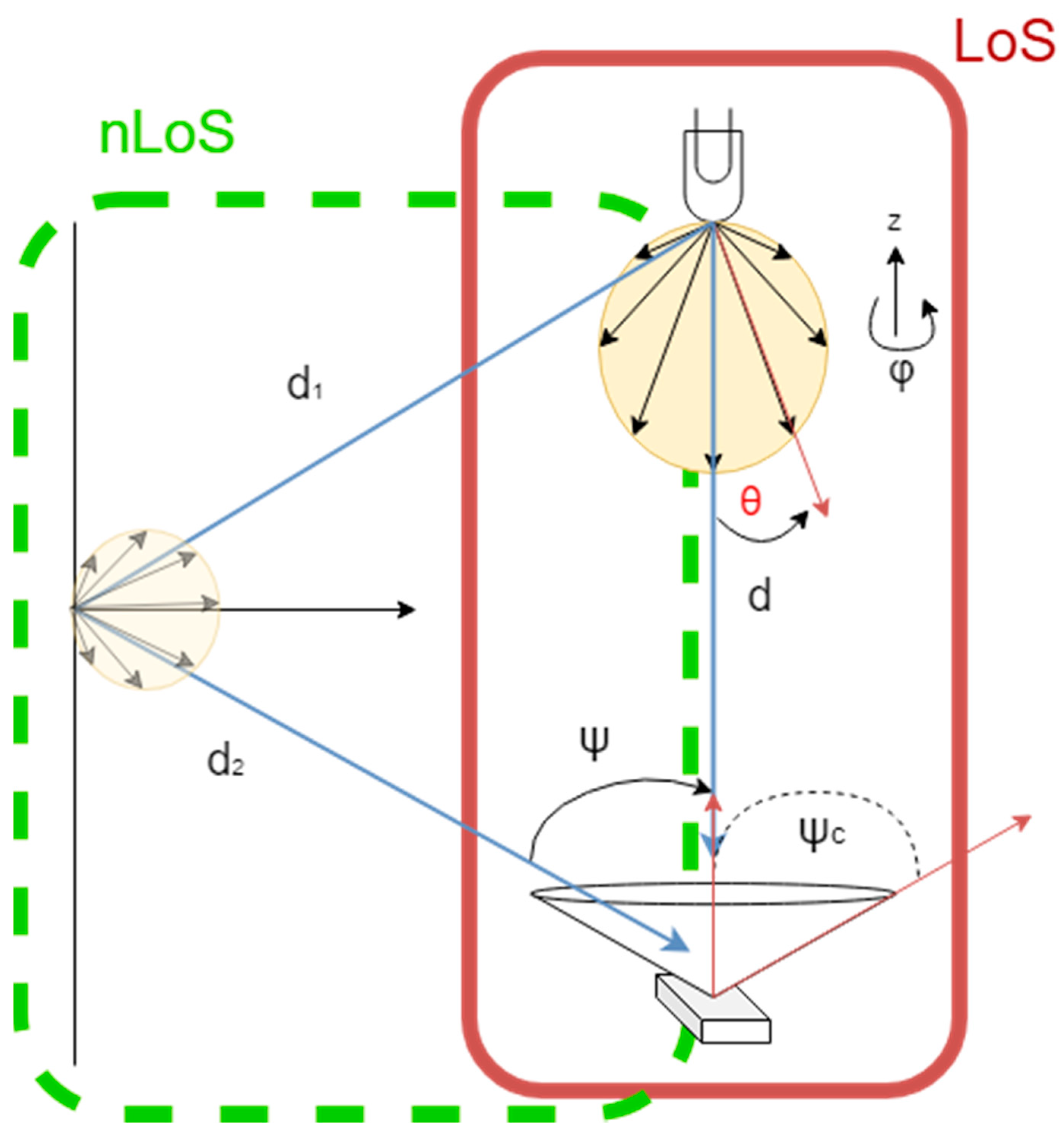
2.1. Visible Light Communication Channel Model
2.2. Atmospheric and Smoke Particle Theory
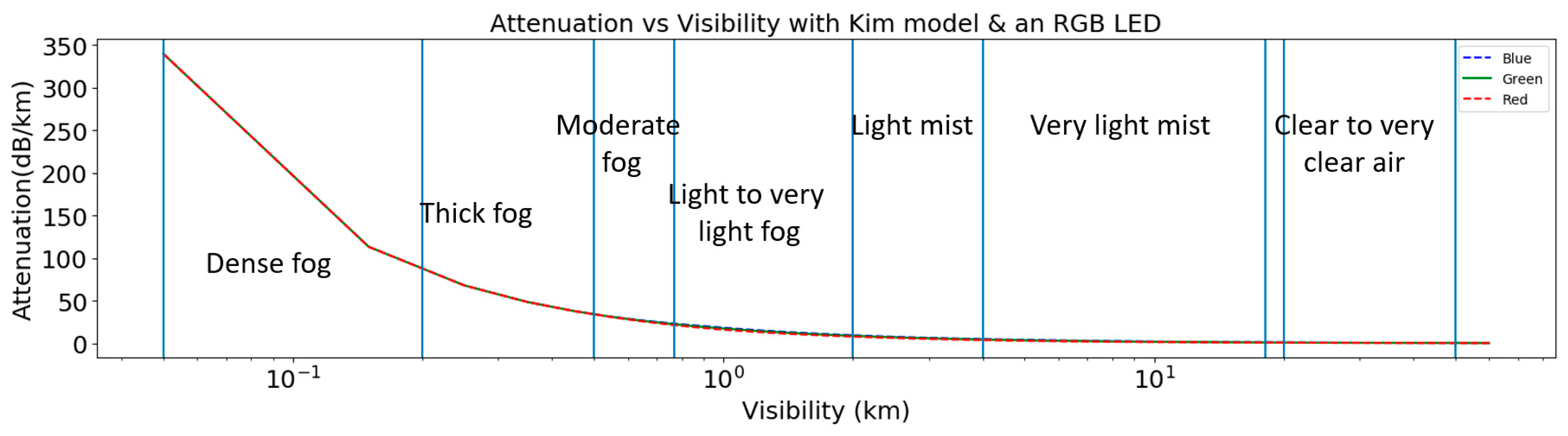
2.2.1. Atmospheric Attenuation
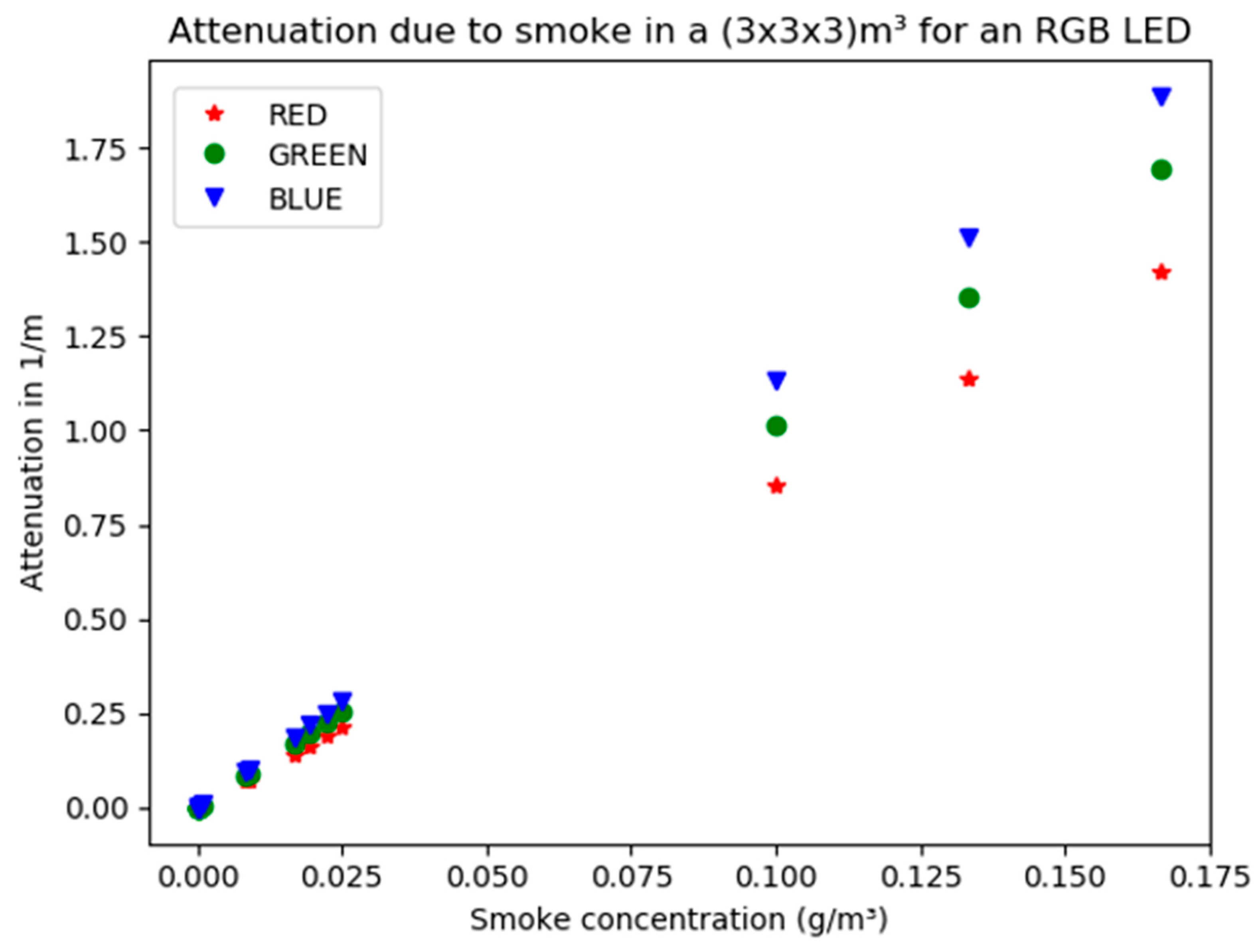
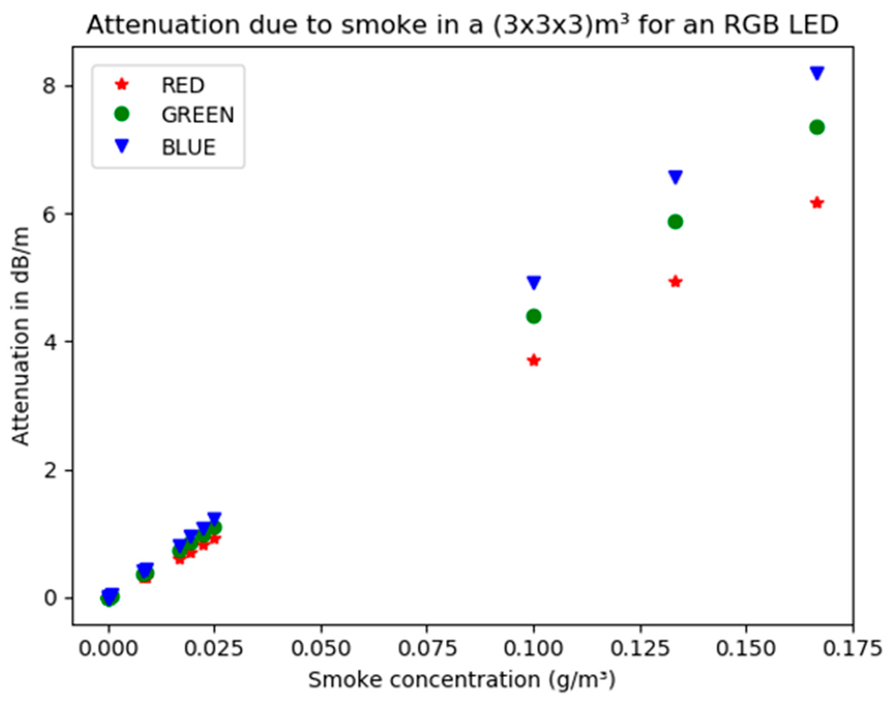
2.2.2. Smoke Attenuation
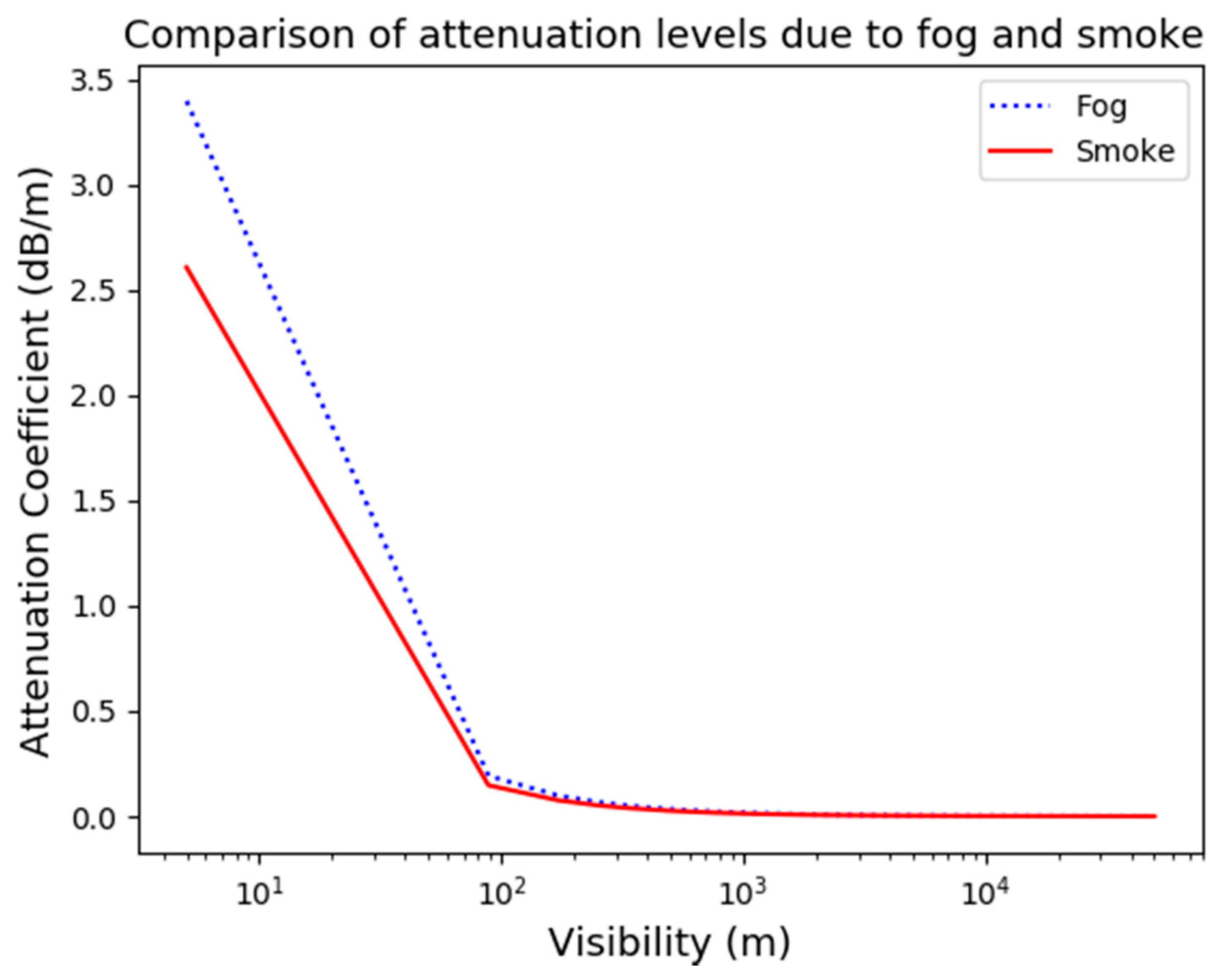
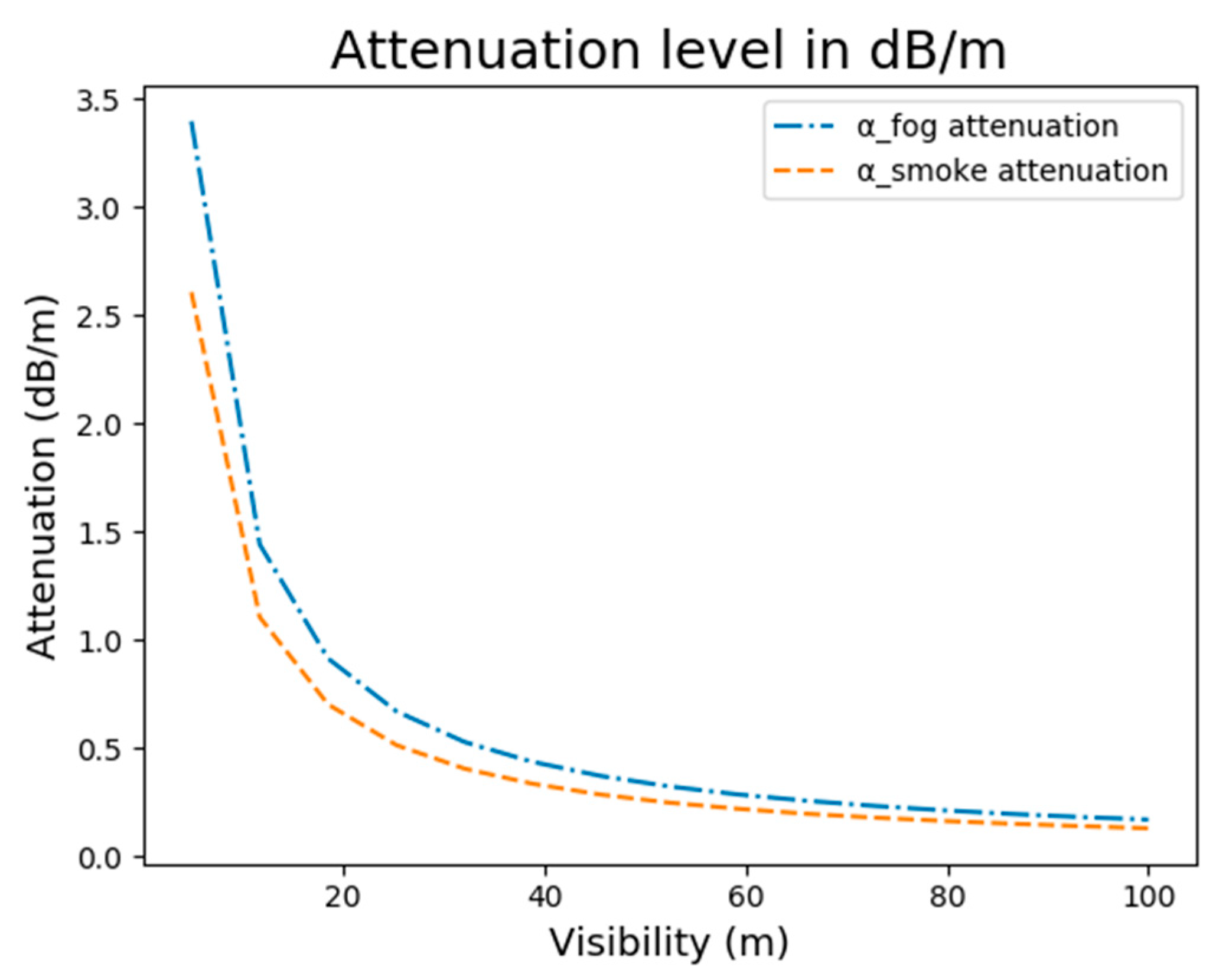
2.2.3. Comparison of Attenuation Levels
3. Materials and Methods
3.1. State of the Art of Channel Modeling Techniques
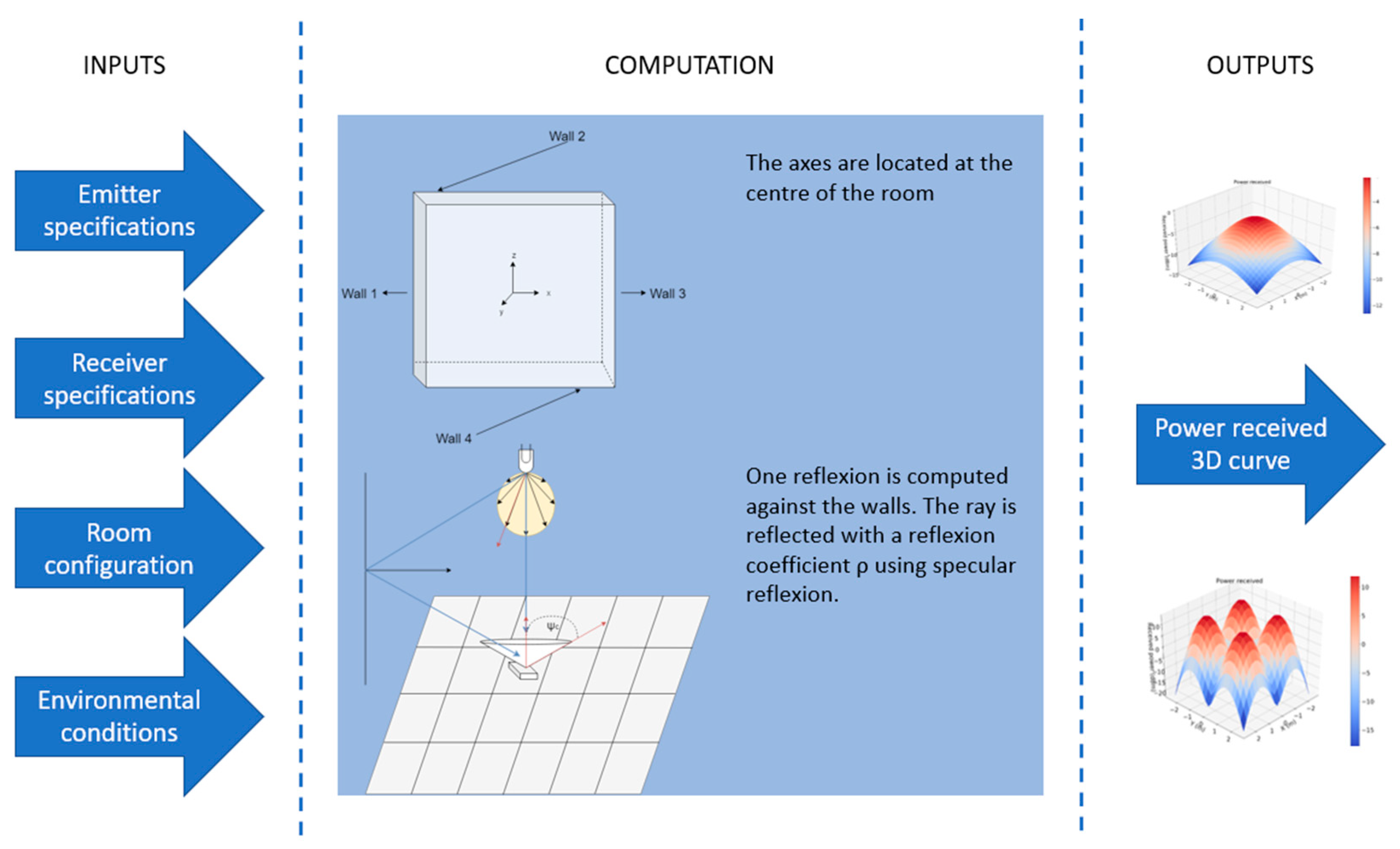
3.2. Methodology Used to Develop and Assess the Python Simulation Tool
- Only the first reflection on the wall (if any) is considered for the non-line-of-sight (nLoS) component. The type of reflection considered is diffuse.
- If there is any fog or smoke, it is assumed to be uniformly distributed in the room, without transitory time.
- The reflection coefficient of materials is uniform on the whole wall and can be adapted to the envisioned use case.
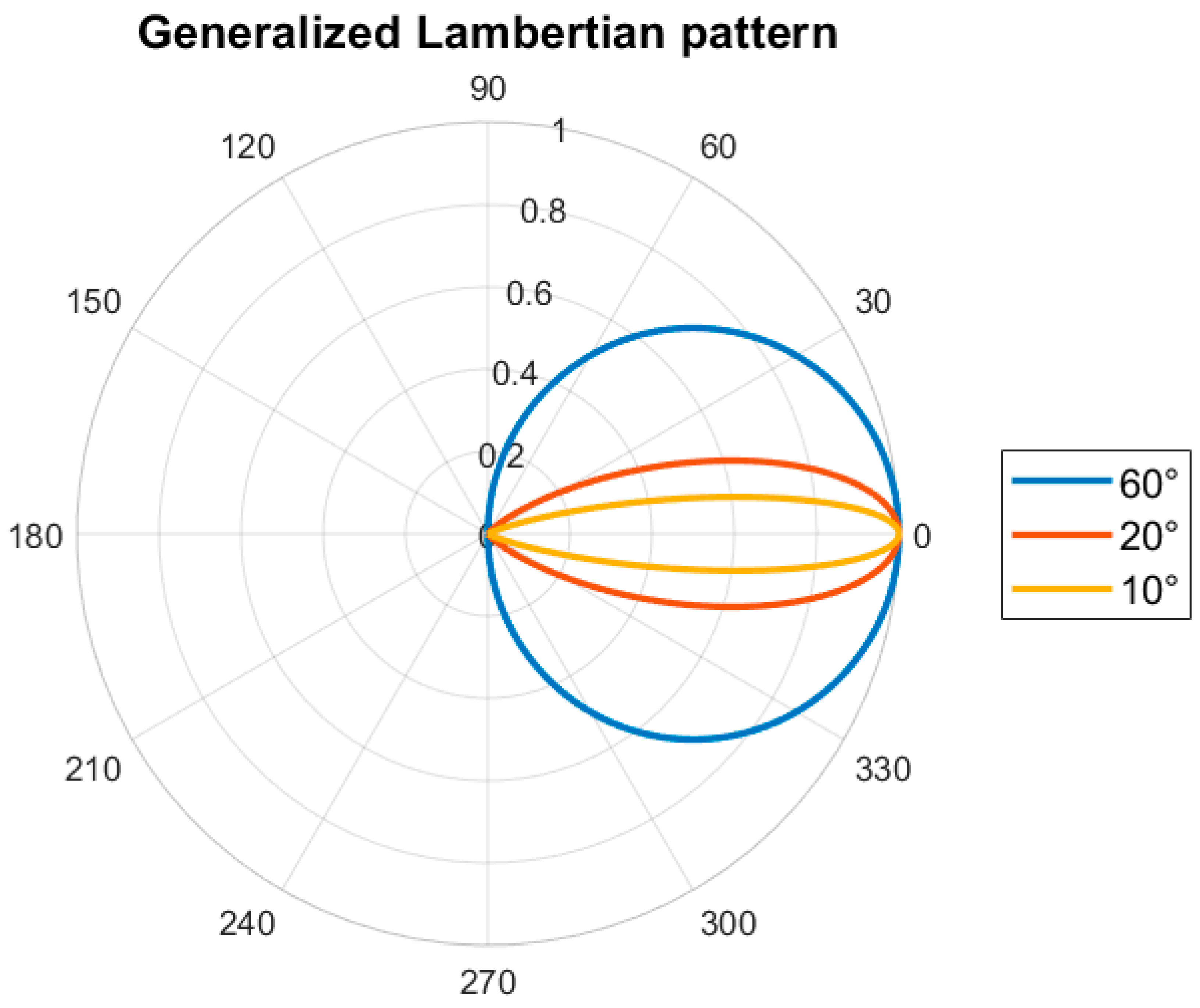
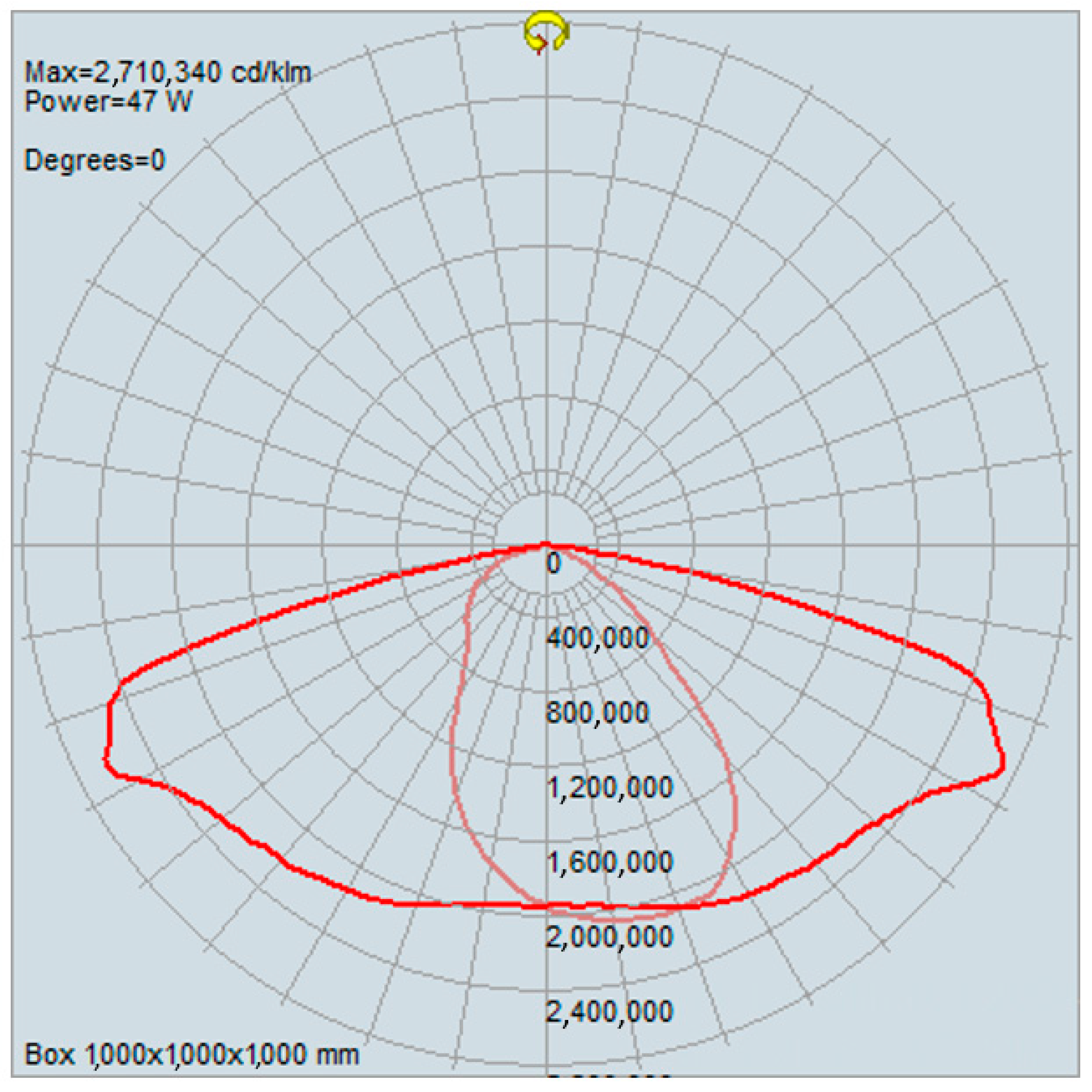
3.3. Radiation Patterns: Lambertian for Scenario 1 and tabulated for Scenario 2
4. Results
5. Discussion
Author Contributions
Funding
Conflicts of Interest
Appendix A

| Aim of the Article | For What | Methodology | Distance | Emitter Used: | Wavelength | Effects | Models Used: |
|---|---|---|---|---|---|---|---|
| Characterize the link margin of an FSO system under different weather conditions [11] | FSO | Simulation: explanation of the effects) | 2.5 km | LASER | 1550 nm | Atmospheric effects (absorption, etc.) | Kim for foggy media |
| Characterization of Fog and Smoke Attenuation in a Laboratory Chamber [12] | FSO | Experiments and proposal of a model | 5.5 m | LASER | 600 to 1600 nm | Fog and smoke in a laboratory chamber | New models developed to match experiments |
| Analysis of a setup put outside measurements [13] | FSO | Experimental and analysis | 80 m–2700m | LASER | 785–850–950 nm | Fog and snow | Analytical model from experiments |
| Performance analysis (power received, SNR, BER) [14] | FSO | Theoretical analysis | Up to 1.5 km | LASER | 650, 850, 950, and 1550 | Fog | Comparison of fog models |
| Channel model of traffic light [18] | VLC (V2I) | Experimental and analytical model drawn | 5–80 m | Traffic light LED | Visible | Sunlight | Analytical model proposed after measurements |
| Demonstration of an outdoor system using a specific type of modulation [19] | VLC (V2V) | Experimental | 100 m | LED | R–G–B: 620–520–470 nm | None | Not applicable |
| Model closed form channel model for V2V [15] | VLC (V2V) | Simulation: ZEMAX | 10 m | Automotive white LED | Visible | scattering | Mie scattering |
| Overview of the VLC technology for outdoor [16] | VLC | Theoretical | Not applicable | LED and laser diodes | Visible | 4 scenarios of outdoor weather | Can be Kim model |
| Signal attenuation measurement in a controlled smoke environment [20] | VLC | Experimental measurement | 30 cm | White LED | Visible | Smoke generated from | Measurements |
| Study of snow and rain effect on a VLC and modulation techniques in terms of SNR, power received and BER, max coverage [17] | VLC (V2I) | Simulation | Up to 300 m | LED | 505 nm | Rain and snow | Marshall, France and Japan rain models |
| Quantify the effects of weather variabilities and smoke on a VLC smart city use case (this paper) | VLC | PYTHON simulator | Up to 8.13 m | LED | 450 nm | Fog and smoke | Kim model (fog) and fire engineering models for smoke |
References
- Kavehrad, M.; Chowdhury, M.I.S. An archipelago of high-bandwidth islands by optical wireless systems—A solution to the USA wireless airwaves spectrum crunch. In Proceedings of the 2012 IEEE Photonics Society Summer Topical Meeting Series, Seattle, WA, USA, 9–11 July 2012; pp. 92–93. [Google Scholar] [CrossRef]
- Kavehrad, M. Optical wireless applications: A solution to ease the wireless airwaves spectrum crunch. In Broadband Access Communication Technologies Vii; International Society for Optics and Photonics: San Francisco, CA, USA, 2013; p. 86450G. [Google Scholar] [CrossRef]
- Ayyash, M.; Elgala, H.; Khreishah, A.; Jungnickel, V.; Little, T.; Shao, S.; Rahaim, M.; Schulz, D.; Hilt, J.; Freund, R. Coexistence of WiFi and LiFi toward 5G: Concepts, opportunities, and challenges. IEEE Commun. Mag. 2016, 54, 64–71. [Google Scholar] [CrossRef]
- Ghassemlooy, Z.; Alves, L.N.; Zvanovec, S.; Khalighi, M.-A. Visible Light Communications; CRC Press: Boca Raton, FL, USA, 2017; p. 591. [Google Scholar]
- Figueiredo, M.; Alves, L.N.; Ribeiro, C. Lighting the Wireless World: The Promise and Challenges of Visible Light Communication. IEEE Consum. Electron. Mag. 2017, 6, 28–37. [Google Scholar] [CrossRef]
- Haas, H.; Yin, L.; Wang, Y.; Chen, C. What is LiFi? J. Light. Technol. 2016, 34, 1533–1544. [Google Scholar] [CrossRef]
- Riurean, S.; Olar, M.; Ionică, A.; Pellegrini, L. Visible Light Communication and Augmented Reality for Underground Positioning System. MATEC Web Conf. 2020, 305, 89. [Google Scholar] [CrossRef]
- Jungnickel, V.; Riege, M.; Wu, X.; Singh, R.; O’Brien, D.C.; Collins, S.; Faulkner, F.; Vazquez, M.M.; Bech, M.; Geilhardt, F.; et al. Enhance Lighting for the Internet of Things. In Proceedings of the 2019 Global LIFI Congress (GLC), Paris, France, 12–13 June 2019; pp. 1–6. [Google Scholar] [CrossRef]
- Alkholidi, A.G.; Altowij, K.S. Free Space Optical Communications—Theory and Practices. In Contemporary Issues in Wireless Communications; Khatib, M., Ed.; InTech: London, UK, 2014. [Google Scholar]
- Ghassemlooy, Z.; Popoola, W.; Rajbhandari, S. Optical Wireless Communications: System and Channel Modelling with MATLAB; Taylor & Francis: Boca Raton, FL, USA, 2013. [Google Scholar]
- Saleem, Z. Free space optical (FSO) link design under diverse weather conditions. WSEAS Trans. Electron. 2006, 3, 225–232. [Google Scholar]
- Ijaz, M.; Ghassemlooy, Z.; Pesek, J.; Fiser, O.; le Minh, H.; Bentley, E. Modeling of Fog and Smoke Attenuation in Free Space Optical Communications Link Under Controlled Laboratory Conditions. J. Light. Technol. 2013, 31, 1720–1726. [Google Scholar] [CrossRef]
- Awan, M.S.; Csurgai-Horváth, L.; Muhammad, S.S.; Leitgeb, E.; Nadeem, F.; Khan, M.S. Characterization of fog and snow attenuations for free-space optical propagation. JCM 2009, 4, 533–545. [Google Scholar] [CrossRef]
- Ali, M.A.A. Performance analysis of fog effect on free space optical communication system. IOSR J. Appl. Phys. 2015, 7, 16–24. [Google Scholar]
- Elamassie, M.; Karbalayghareh, M.; Miramirkhani, F.; Kizilirmak, R.C.; Uysal, M. Effect of fog and rain on the performance of vehicular visible light communications. In Proceedings of the 2018 IEEE 87th Vehicular Technology Conference (VTC Spring), Porto, Portugal, 3–6 June 2018; pp. 1–6. [Google Scholar]
- Ndjiongue, A.R.; Ferreira, H.C. An overview of outdoor visible light communications: An overview of outdoor visible light communications. Trans. Emerg. Telecommun. Technol. 2018, 29, e3448. [Google Scholar] [CrossRef]
- Zaki, R.W.; Fayed, H.A.; el Aziz, A.A.; Aly, M.H. Outdoor Visible Light Communication in Intelligent Transportation Systems: Impact of Snow and Rain. Appl. Sci. 2019, 9, 5453. [Google Scholar] [CrossRef]
- Cui, K.; Chen, G.; Xu, Z.; Roberts, R.D. Traffic light to vehicle visible light communication channel characterization. Appl. Opt. 2012, 51, 6594–6605. [Google Scholar] [CrossRef] [PubMed]
- Zhao, J.; Zhang, M.; Liang, S.; Ding, J.; Wang, F.; Lu, X.; Wang, C.; Chi, N. 100-m field trial for 5G wireless backhaul based on circular (7,1) 8-QAM modulated outdoor visible light communication. In Proceedings of the 2017 Opto-Electronics and Communications Conference (OECC) and Photonics Global Conference (PGC), Singapore, 31 July–4 August 2017; pp. 1–4. [Google Scholar] [CrossRef]
- Xie, R.; Li, Z.; Gu, E.; Huang, Q. Signal attenuation of visible light communication in smoke environment. Opt. Eng. 2019, 58, 1. [Google Scholar] [CrossRef]
- Esmail, M.A.; Fathallah, H.; Alouini, M.-S. Outdoor FSO Communications under Fog: Attenuation Modeling and Performance Evaluation. IEEE Photonics J. 2016, 8, 1–22. [Google Scholar] [CrossRef]
- Hurley, M.J.; Gottuk, D.T.; Hall, J.R., Jr.; Harada, K.; Kuligowski, E.D.; Puchovsky, M.; Torero, J.L.; Watts, J.M., Jr.; Wieczorek, C.J. (Eds.) SFPE Handbook of Fire Protection Engineering; Springer: New York, NY, USA, 2016. [Google Scholar]
- Dimitrov, S.; Haas, H. Principles of LED Light Communications: Towards Networked Li-Fi; Cambridge University Press: Cambridge, UK, 2015; p. 228. [Google Scholar]
- Burchardt, H.; Serafimovski, N.; Tsonev, D.; Videv, S.; Haas, H. VLC: Beyond point-to-point communication. IEEE Commun. Mag. 2014, 52, 98–105. [Google Scholar] [CrossRef]
- NIKKON. Datasheet 45W LED STREET LANTERN (3000K) MURA S NIKKON. Available online: https://lumsearch.com/fr/article/Z4uKfIZtRYKEYL-xqyHFNQ (accessed on 15 October 2020).
- Hoeher, A.P. Visible Light Communications: Theoretical and Practical Foundations; Carl Hanser Verlag: Munich, Germany, 2019. [Google Scholar]
- Moreno, I.; Avendaño-Alejo, M.; Saucedo-A, T.; Bugarin, A. Modeling LED street lighting. Appl. Opt. 2014, 53, 4420. [Google Scholar] [CrossRef] [PubMed]
- Ding, D.; Ke, X. A new indoor VLC channel model based on reflection. Optoelectron. Lett. 2010, 6, 295–298. [Google Scholar] [CrossRef]
- Chung, Y.H.; Oh, S. Efficient optical filtering for outdoor visible light communications in the presence of sunlight or articifical light. In Proceedings of the 2013 International Symposium on Intelligent Signal Processing and Communication Systems, Naha-shi, Japan, 12–15 November 2013; pp. 749–752. [Google Scholar] [CrossRef]
- Islim, M.S.; Videv, S.; Safari, M.; Xie, E.; McKendry, J.J.D.; Gu, E.; Dawson, M.D.; Haas, H. The Impact of Solar Irradiance on Visible Light Communications. J. Light. Technol. 2018, 36, 2376–2386. [Google Scholar] [CrossRef]
- Friedlander, S.K. Smoke, Dust, and Haze Fundamentals of Aerosol Dynamics, 2nd ed.; Oxford University Press: Oxford, UK; New York, NY, USA, 2000. [Google Scholar]
- Cojan, Y. Propagation du rayonnement dans l’atmosphère. Tech. L’ingénieur Electron. 1995, 6, 35. [Google Scholar]
- Gupta, R.; Aggarwal, A. Fog and Atmospheric Turbulence in FSO: Models to mitigate. Int. J. Contemp. Technol. Res. 2019, 2, 3. [Google Scholar] [CrossRef]
- Kim, I.I.; McArthur, B.; Korevaar, E.J. Comparison of laser beam propagation at 785 nm and 1550 nm in fog and haze for optical wireless communications. In Optical Wireless Communications III; International Society for Optics and Photonics: Boston, MA, USA, 2001; pp. 26–37. [Google Scholar] [CrossRef]
- Mulholland, G.W.; Fernandez, M. The Basis for a Smoke Concentration Measurement Using Light Extinction. In Proceedings of the 2nd International Conference on Fire Research and Engineering, Gaithersburg, ML, USA, 3–8 August 1997. [Google Scholar]
- Putorti, A.D., Jr. Design Parameters for Stack-Mounted Light Extinction Measurement Devices; NASA: Washington, DC, USA, 1999. [Google Scholar]
- Widmann, J.F.; Yang, J.C.; Smith, T.J.; Manzello, S.L.; Mulholland, G.W. Measurement of the optical extinction coefficients of post-flame soot in the infrared. Combust. Flame 2003, 134, 119–129. [Google Scholar] [CrossRef]
- Mulholland, G.W.; Croarkin, C. Specific extinction coefficient of flame generated smoke. Fire Mater. 2000, 24, 227–230. [Google Scholar] [CrossRef]
- Babrauskas, V.; Grayson, S.J. Heat Release in Fires; Taylor & Francis: Abingdon, UK, 1990. [Google Scholar]
- Mulholland, G.W.; Johnsson, E.L.; Fernandez, M.G.; Shear, D.A. Design and testing of a new smoke concentration meter. Fire Mater. 2000, 24, 231–243. [Google Scholar] [CrossRef]
- Jin, T.; Yamada, T. Irritating effects of fire smoke on visibility. Fire Sci. Technol. 1985, 5, 79–90. [Google Scholar] [CrossRef]
- Jin, T. Visibility and human behavior in fire smoke. In SFPE Handbook of Fire Protection Engineering; Springer: Berlin/Heidelberg, Germany, 2002; Volume 2, pp. 42–53. [Google Scholar]
- Seader, J.; Einhorn, I. Some physical, chemical, toxicological, and physiological aspects of fire smokes. Symp. Combust. 1977, 16, 1423–1445. [Google Scholar] [CrossRef]
- Luo, P.; Zhang, M.; Ghassemlooy, Z.; Le Minh, H.; Tsai, H.-M.; Tang, X.; Png, L.C.; Han, D. Experimental Demonstration of RGB LED-Based Optical Camera Communications. IEEE Photonics J. 2015, 7, 1–12. [Google Scholar] [CrossRef]
- Gfeller, F.R.; Bapst, U. Wireless in-house data communication via diffuse infrared radiation. Proc. IEEE 1979, 67, 1474–1486. [Google Scholar] [CrossRef]
- Barry, J.R.; Kahn, J.M.; Krause, W.J.; Lee, E.A.; Messerschmitt, D.G. Simulation of multipath impulse response for indoor wireless optical channels. IEEE J. Sel. Areas Commun. 1993, 11, 367–379. [Google Scholar] [CrossRef]
- Khan, M.W.; Mehr-e-Munir, U.F.; Amer, A. Analysis of Key Transmission Issues in Optical Wireless Communication for Indoor and Outdoor Applications. Int. J. Comput. Sci. Inf. Secur. 2018, 16, 3. [Google Scholar]
- Sarbazi, E.; Uysal, M.; Abdallah, M.; Qaraqe, K. Ray tracing based channel modeling for visible light communications. In Proceedings of the 2014 22nd Signal Processing and Communications Applications Conference (SIU), Trabzon, Turkey, 23–25 April 2014; pp. 702–705. [Google Scholar]
- Rodríguez, S.; Mendoza, B.; Miranda, G.; Segura, C.; Jiménez, R.P. Simulation of impulse response for indoor wireless optical channels using 3D CAD models. SPIE Microtechnol. 2011, 8067, 80670A. [Google Scholar]
- Jovicic, A.; Li, J.; Richardson, T. Visible light communication: Opportunities, challenges and the path to market. IEEE Commun. Mag. 2013, 51, 26–32. [Google Scholar] [CrossRef]
- Quimby, R.S. Photonics and Lasers: An Introduction; John Wiley & Sons: Hoboken, NJ, USA, 2006. [Google Scholar]
- Nassar, M.A.; Luxford, L.; Cole, P.; Oatley, G.; Koutsakis, P. The current and future role of smart street furniture in smart cities. IEEE Commun. Mag. 2019, 57, 68–73. [Google Scholar] [CrossRef]
- Bodart, M.; de Peñaranda, R.; Deneyer, A.; Flamant, G. Photometry and colorimetry characterisation of materials in daylighting evaluation tools. Build. Environ. 2008, 43, 2046–2058. [Google Scholar] [CrossRef]
- Mackowiak, V.; Peupelmann, J.; Ma, Y.; Gorges, A. NEP–Noise Equivalent Power; Thorlabs Inc.: Newton, NJ USA, 2015. [Google Scholar]


| Type | Smoke Conversion Factor, | Combustion Conditions |
|---|---|---|
| Douglas fir | 0.010–0.025 | Flaming |
| Hardboard | 0.0004–0.0010 | Flaming |
| Fiberboard | 0.005–0.010 | Flaming |
| Polyvinylchloride | 0.12 | Flaming |
| Polyurethane (flexible) | 0.010–0.035 | Flaming |
| Polyurethane (rigid) | 0.09 | Flaming |
| Polystyrene | 0.15–0.17 | Flaming |
| Polypropylene | 0.080–0.016 | Flaming |
| Polymethylmethacrylate | 0.02 | Flaming |
| Polyoxymethylene | 0 | Flaming |
| Cellulosic insulation | 0.01–0.12 | Smoldering |
| Software | MATLAB | OptiSystem | Zemax | CAD |
|---|---|---|---|---|
| Type of emitter | White or IR LED | White or IR LED | White LED | White LED |
| Radiation pattern | Lambertian | Lambertian | Realistic | Adaptive |
| CIR 1 model | Geometric optics | Geometric optics | Monte Carlo Ray Tracing | Modified Monte Carlo ray Tracing |
| Phenomena | Single diffuse Reflection | Reflection | Diffuse and specular reflection | Reflection, absorption, refraction |
| Parameters | Bus Stop | House’s Side | |
|---|---|---|---|
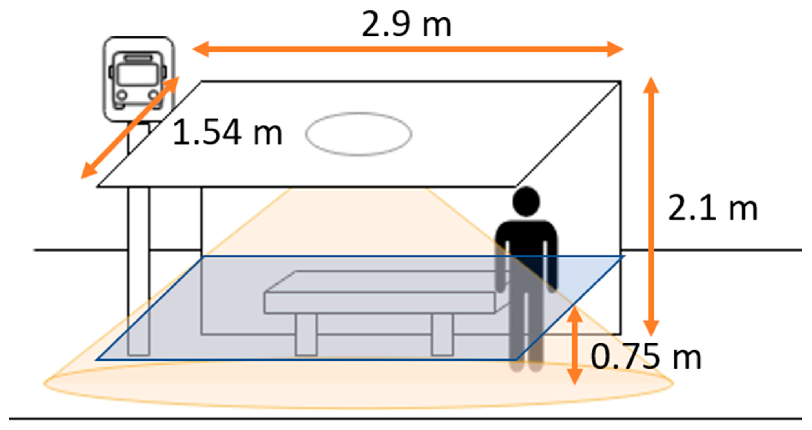
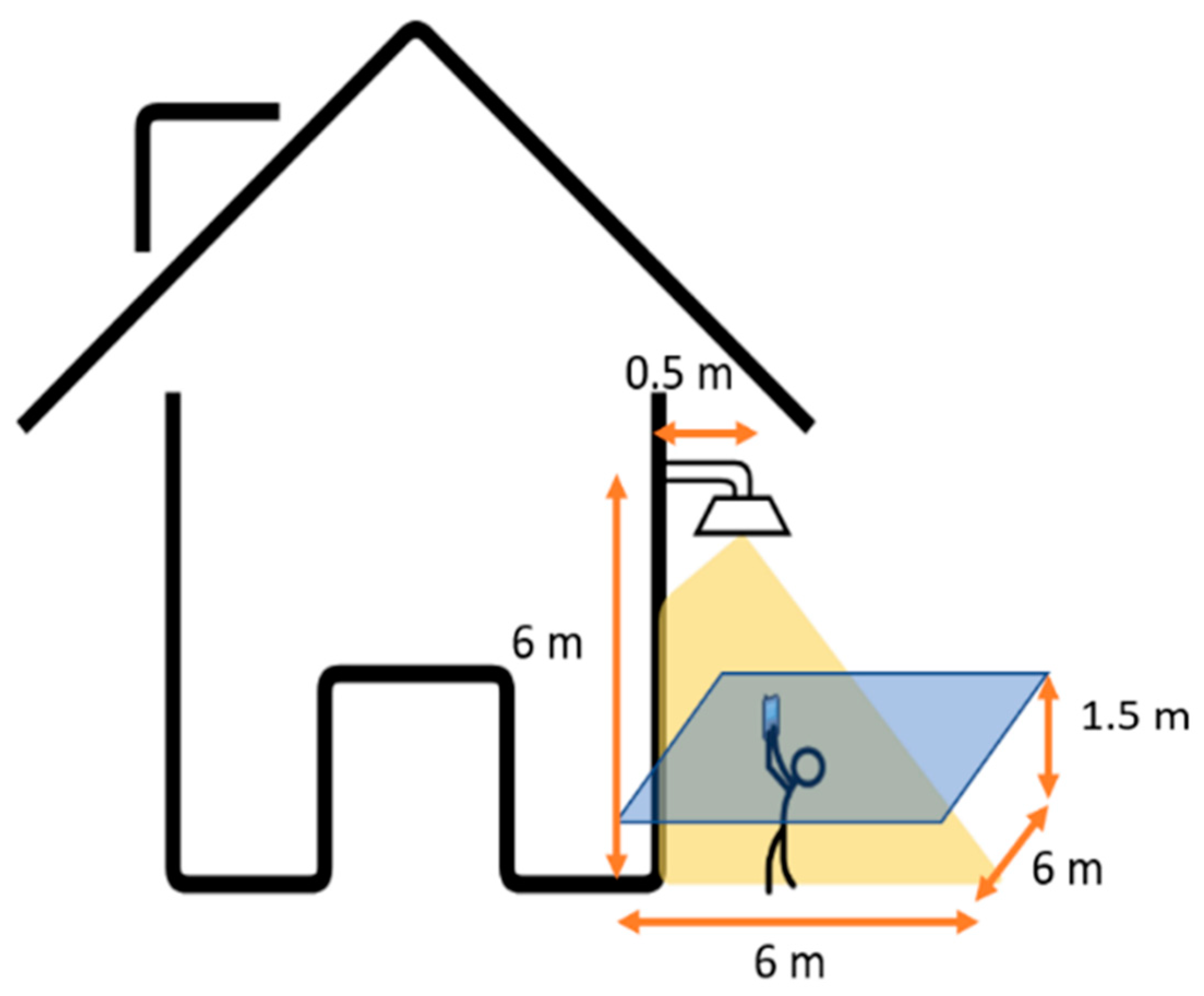
| Emitter | Location | Center ceiling | Center top wall (head 0.5 m from wall) |
| Half power angle | 60° | 60° | |
| Power emitted | 2 Watts | 47 Watts | |
| Receiver | Field of View | 60° | 60° |
| Receiving area | 13 mm² | 13 mm² | |
| Refractive index | 1.5 | 1.5 | |
| Environment | Size of the space | 2.9 × 2.1 × 1.54 m³ | 6 × 6 × 6 m³ |
| Number of walls | 1 | 1 | |
| Precision of the mesh | 72 × 52 | 50 × 50 | |
| Height of the receiver plane (from ground) | 0.75 m | 1.5 m |
| Parameters | Bus Stop | House’s Side |
|---|---|---|
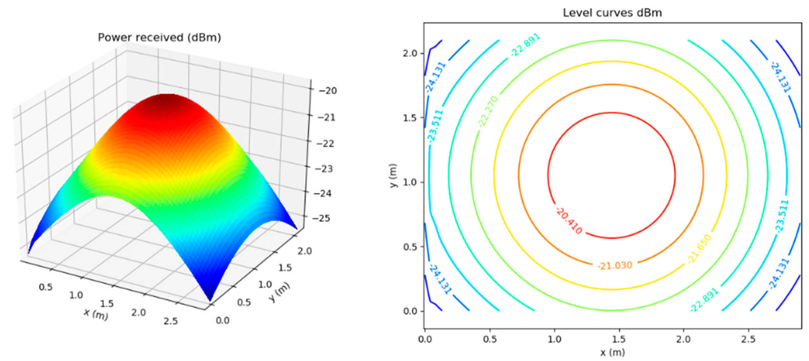
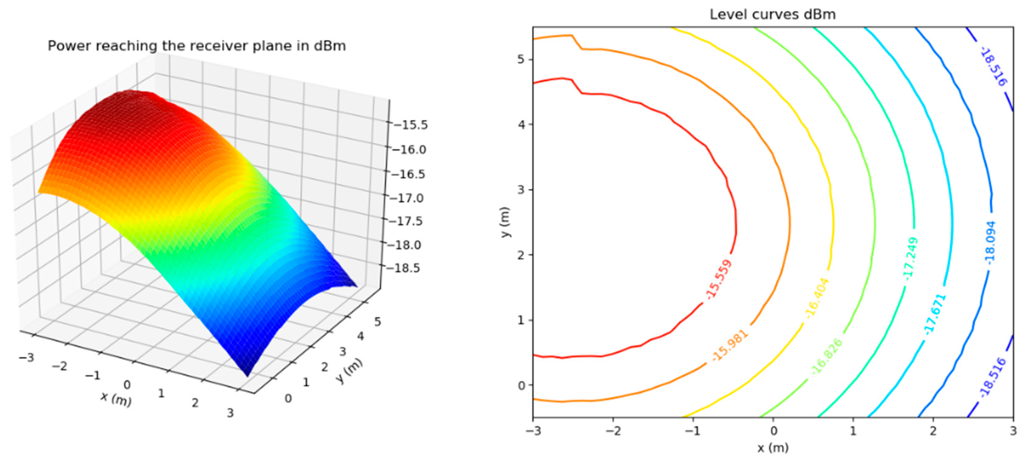
| Max power | −19.79 dBm | −15.14 dBm |
| Min power | −25.37 dBm | −18.94 dBm |
| Mean power | −22.10 dBm | −16.52 dBm |
| Parameters | Bus Station | House’s Side |
|---|---|---|
| Longest distance | 2.12 m | 6.74 m |
| for and | 12.72 dB | 40.45 dB |
| for and | 0.63 dB | 2.02 dB |
Publisher’s Note: MDPI stays neutral with regard to jurisdictional claims in published maps and institutional affiliations. |
© 2020 by the authors. Licensee MDPI, Basel, Switzerland. This article is an open access article distributed under the terms and conditions of the Creative Commons Attribution (CC BY) license (http://creativecommons.org/licenses/by/4.0/).
Share and Cite
Georlette, V.; Bette, S.; Brohez, S.; Pérez-Jiménez, R.; Point, N.; Moeyaert, V. Outdoor Visible Light Communication Channel Modeling under Smoke Conditions and Analogy with Fog Conditions. Optics 2020, 1, 259-281. https://doi.org/10.3390/opt1030020
Georlette V, Bette S, Brohez S, Pérez-Jiménez R, Point N, Moeyaert V. Outdoor Visible Light Communication Channel Modeling under Smoke Conditions and Analogy with Fog Conditions. Optics. 2020; 1(3):259-281. https://doi.org/10.3390/opt1030020
Chicago/Turabian StyleGeorlette, Véronique, Sébastien Bette, Sylvain Brohez, Rafael Pérez-Jiménez, Nicolas Point, and Véronique Moeyaert. 2020. "Outdoor Visible Light Communication Channel Modeling under Smoke Conditions and Analogy with Fog Conditions" Optics 1, no. 3: 259-281. https://doi.org/10.3390/opt1030020
APA StyleGeorlette, V., Bette, S., Brohez, S., Pérez-Jiménez, R., Point, N., & Moeyaert, V. (2020). Outdoor Visible Light Communication Channel Modeling under Smoke Conditions and Analogy with Fog Conditions. Optics, 1(3), 259-281. https://doi.org/10.3390/opt1030020