Inverse Uncertainty Quantification in Material Parameter Calibration Using Probabilistic and Interval Approaches

Abstract

In model calibration, the identification of the unknown parameter values themselves, but also the uncertainty of these model parameters, due to uncertain measurements or model outputs might be required. The analysis of parameter uncertainty helps us understand the calibration problem better. Investigations on the parameter sensitivity and the uniqueness of the identified parameters could be addressed within uncertainty quantification. In this paper, we investigate different probabilistic approaches for this purpose, which identify the unknown parameters as multivariate distribution functions. However, these approaches require accurate knowledge of the model output covariance, which is often not available. In addition, we investigate interval optimization methods for the identification of parameter bounds. The correlation or interaction of the input parameters can be modeled with a convex feasible domain that belongs to a feasible solution of the model output within given bounds. We introduce a novel radial line-search procedure that can identify the boundary of such a parameter domain for arbitrary nonlinear dependencies between model input and output.

1. Introduction

Within the calibration of material models, the numerical results of a simulation model are compared with the experimental measurements. One common approach is to minimize the squared errors between the simulation response and the measurements, the so-called least squares approach [1]. This minimization task can be solved using a single-objective optimization algorithm to obtain the optimal parameter set. The optimization procedure requires special attention if the optimization task is not convex and contains several local minima, as discussed in [2]. A recent overview of optimization techniques applied to solving a calibration task is given in [3,4]. Often, a maximum likelihood approach [1] is used to formulate the optimization goal. To ensure a successful identification with optimization techniques, the sensitivity of the model parameters with respect to the considered model outputs should be investigated initially, as discussed in [5].

In addition to the parameter values themselves, the estimation of the parameter uncertainty due to scatter in the experimental measurements and inherent randomness of the material properties requires further investigations. Generally, probabilistic and non-probabilistic techniques have been developed to estimate parameter uncertainty [6]. A well-known probabilistic method is the maximum likelihood approach [1,7], which uses straightforward linearization to represent the parameter scatter as a multivariate normal distribution. A generalization of this method is the Bayesian updating technique [1], where the joint distribution function of the model parameters could also be non-normal, but can be obtained only implicitly from the model input–output dependencies in the general case. A good overview of recent developments with this technique is given, e.g., in [8,9,10,11]. Since the parameter distribution function can be obtained in closed form only for special cases, inverse sampling procedures such as Markov Chain Monte Carlo (MCMC) methods are usually applied to generate discrete samples of the unknown multidimensional parameter distribution [12]. Most of these methods rely on the original Metropolis–Hastings algorithm [13]. However, the MCMC methods usually require a large number of model evaluations, and surrogate models are often applied to reduce the numerical burden of the identification procedure [2,14]. Recent developments utilize Bayesian neural networks to represent the forward simulation model, including the corresponding parameter and responses uncertainty in a probabilistic approximation model [15,16,17]. As an alternative to the ordinary least squares formulation, Kalman filter identification has been introduced [18] and recently applied for material parameter identification in [19,20]. This technique is a Bayesian estimator that uses prior information to identify the parameters. However, all the mentioned probabilistic methods require an accurate estimate of the measurement covariance matrix, which is often not available.

In addition to probabilistic methods, interval approaches have been developed that model the uncertainty of the model inputs and outputs as interval numbers [21,22] or confidence sets [23]. Based on this assumption, interval predictor models have been used for model parameter identification [24]. The unknown model parameter bounds can be obtained for inverse problems from the given model output bounds using interval optimization methods [25,26]. In [27], interval optimization was introduced for fuzzy numbers to obtain a quasi-density of unknown model outputs in forward problems. However, this method can also be applied to inverse problems, which usually results in minimum and maximum values for each parameter considered in the model calibration. In [28,29], bounding boxes were used to represent the multidimensional domain of the feasible input parameter space. This idea has been extended quite recently to consider correlations between the model parameters [30,31].

In the rest of this paper, we investigate different methods to estimate the uncertainty of the calibrated parameters from given measurement uncertainty. In using the classical probabilistic approaches as the maximum likelihood estimator and the Bayesian updating procedure as benchmark methods, the scatter of the identified parameters is estimated as a multivariate probability density function. Furthermore, we present an interval-based approach by assuming the scatter of the measurements not as correlated random numbers but as individual intervals with known minimum and maximum values. The corresponding possible minimum and maximum values for each input parameter will be obtained using a constrained optimization procedure. Furthermore, the identification of the whole feasible parameter domain for the given measurement bounds is obtained using a novel radial line-search method, which is extended for more than two model parameters using Fekete point sets on a unit hypersphere. With the help of this approach, a uniform discretization of the feasible parameter domain boundary is obtained. Furthermore, we emphasize the initial sensitivity analysis, which should be considered for all approaches to neglect unimportant parameters in the calibration procedure. As numerical examples, we identify first the material parameters of a bilinear elasto-plasticity model and second the fracture parameters of plain concrete based on a wedge splitting test.

2. Materials and Methods

Within the calibration of material models, the numerical results of a simulation model $\mathbf{y}\left(\mathbf{p}\right)$ are compared with the experimental measurements ${\mathbf{y}}^{*}$, as illustrated in Figure 1. One common approach is to minimize the squared errors between the simulation response and the measurements, the so-called least squares approach [1]:

$${\left[{\mathbf{y}}^{*}-\mathbf{y}\left(\mathbf{p}\right)\right]}^T\left[{\mathbf{y}}^{*}-\mathbf{y}\left(\mathbf{p}\right)\right]\to min.$$

(1)

This minimization task can be solved with a single-objective optimization algorithm to obtain the optimal parameter set ${\mathbf{p}}_{opt}$. The optimization procedure requires special attention if the optimization task is not convex and contains several local minima, as discussed in [2].

2.1. Sensitivity Analysis of the Forward Problem

In order to obtain a sufficient accuracy of the calibrated model parameters, a certain sensitivity of these parameters with respect to the model responses is necessary. If all model responses are not sensitive with respect to a specific parameter, this parameter cannot be identified within an inverse approach. In such a case, a non-sensitive parameter should be kept fixed and not considered in the calibration process.

A quite common approach for sensitivity analysis is the global variance-based method using Sobol indices [32,33]. In this method, the contribution of the variation in the input parameters with respect to the variation in a certain model output can be analyzed. Originally, this method was introduced for sensitivity analysis in the context of uncertainty quantification, but it can similarly apply for optimization problems, as discussed in [34]. If we define lower and upper bounds for the m unknown model parameters $p_j$

$$p_i^l\le p_i\le p_i^u,i=1,\dots ,m,$$

(2)

we can assume a uniform distribution for each parameter

$$P_i\sim \mathcal{U}[p_i^l,p_i^u].$$

(3)

The variance contribution of parameter $P_i$ with respect to a model output $Y_j$ can be quantified with the first-order sensitivity measure introduced by [32]

$$S_{P_i}\left(Y_j\right)={\displaystyle \frac{V_{P_i}\left(E_{{\mathbf{P}}_{\sim i}}\left(Y_j\right|P_i)\right)}{V\left(Y_j\right)}},$$

(4)

where $V\left(Y_j\right)$ is the unconditional variance of $Y_j$, and $V_{P_i}\left(E_{{\mathbf{P}}_{\sim i}}\left(Y_j\right|P_i)\right)$ is called the variance of conditional expectation, with ${\mathbf{P}}_{\sim i}$ denoting the set of all parameters but $P_i$. $V_{P_i}\left(E_{{\mathbf{P}}_{\sim i}}\left(Y_i\right|P_i)\right)$ measures the first-order effect of $P_i$ on the model output. Since first-order sensitivity indices quantify only the decoupled influence of each parameter, the total effect sensitivity indices have been introduced by [33] as follows:

$$S_{P_i}^T\left(Y_j\right)=1-{\displaystyle \frac{V_{{\mathbf{P}}_{\sim i}}\left(E_{P_i}\left(Y_j\right|{\mathbf{P}}_{\sim i})\right)}{V\left(Y_j\right)}},$$

(5)

where $V_{{\mathbf{P}}_{\sim i}}\left(E_{P_i}\left(Y_j\right|{\mathbf{P}}_{\sim i})\right)$ measures the first-order effect of ${\mathbf{P}}_{\sim i}$ on the model output, which does not contain any effect corresponding to $P_i$.

Generally, the computation of $S_i$ and $S_i^T$ requires special estimators with a large number of model evaluations [34]. In [35], regression-based estimators were introduced, which require only a single sample set of the model input parameters and the corresponding model outputs. One very simply estimator for the first-order index is the squared Pearson correlation coefficient

$$S_{P_i}^{corr}\left(Y_j\right)={\rho }^2(P_i,Y_j).$$

(6)

The Pearson correlation assumes a linear dependence between model input and output. If this is fulfilled, the sum of the first-order indices should be close to one. However, if the model output is a strongly nonlinear function of the parameters, the sum is smaller than one, and a reliable estimate is not possible with this approach.

With the Metamodel of Optimal Prognosis (MOP) [35], a more accurate metamodel-based approach for variance-based sensitivity analysis was introduced, where the quality of the metamodel is estimated with the Coefficient of Prognosis (CoP) by means of a sample cross-validation. If the CoP is close to one, the metamodel can represent the main part of the model output variation, and thus, the sensitivity estimates are sufficiently accurate. In the MOP approach, different types of metamodels, such as classical polynomial response surface models [36,37], Kriging [38], Moving Least Squares [39], and artificial neural networks [40] have been tested automatically for a specific model output and evaluated by means of the CoP measure. This approach is available with the Ansys optiSLang software package [41]. Further information on the CoP measure can be found in [42]. Samples for the regression-based estimators can be generated purely randomly within the defined parameter bounds. However, in order to increase the accuracy of the sensitivity estimates, we applied improved Latin Hypercube sampling (LHS) [43], which reduces the spurious correlations between the inputs parameters.

2.2. Maximum Likelihood Approach

In the maximum likelihood approach [1,7], the likelihood of the parameters is defined to be proportional to the conditional probability of the measurements ${\mathbf{y}}^{*}$ for a given parameter set $\mathbf{p}$:

$$L=k·f\left({\mathbf{y}}^{*}\right|\mathbf{p}).$$

(7)

In assuming that the chosen model can represent the material behavior perfectly, the remaining gap between model responses and experimental observations $({\mathbf{y}}^{*}-\mathbf{y})$ can be explained only with measurement errors. In this case, $P\left({\mathbf{y}}^{*}\right|\mathbf{p})$ is equivalent to the probability of reproducing the measurement errors. Assuming a multivariate normal distribution for the measurement errors yields [7]

$$P\left({\mathbf{y}}^{*}\right|\mathbf{p})=P({\mathbf{y}}^{*}-\mathbf{y}\left(\mathbf{p}\right))={\displaystyle \frac{1}{\sqrt{{\left(2\pi \right)}^m\left|{\mathbf{C}}_{\mathbf{yy}}\right|}}}exp\left[-{\displaystyle \frac{1}{2}}{[{\mathbf{y}}^{*}-\mathbf{y}\left(\mathbf{p}\right)]}^T{\mathbf{C}}_{\mathbf{yy}}^{-1}[{\mathbf{y}}^{*}-\mathbf{y}\left(\mathbf{p}\right)]\right],$$

(8)

where ${\mathbf{C}}_{\mathbf{yy}}$ is the covariance matrix of the measurement uncertainty. Maximizing the likelihood L is equivalent to minimizing $S=-2lnL$ and yields the following objective function:

$$J\left(\mathbf{p}\right)={\left[{\mathbf{y}}^{*}-\mathbf{y}\left(\mathbf{p}\right)\right]}^T{\mathbf{C}}_{\mathbf{yy}}^{-1}\left[{\mathbf{y}}^{*}-\mathbf{y}\left(\mathbf{p}\right)\right]\to min.$$

(9)

If the measurement errors $y_i^{*}-y_i$ are assumed to be independent, the objective function equals a weighted least squares formulation:

$$J=\sum _{i=1}^n{w}_i{(y_i^{*}-y_i)}^2,w_i={\displaystyle \frac{1}{{\sigma }_{y,i}^2}},$$

(10)

where the weight factor $w_i$ for each measurement value is the inverse of its variance ${\sigma }_{y,i}^2$. For constant measurement errors, this objective simplifies to the well-known least squares formulation introduced in Equation (1). In this case, the optimal parameter set ${\mathbf{p}}_{opt}$ can be obtained using the maximum likelihood approach with standard optimization procedures without exact knowledge of the measurement covariance matrix.

The objective function in Equation (9) can be linearized as follows [7]:

$$\Delta \mathbf{p}={\left({\mathbf{A}}^T{\mathbf{C}}_{\mathbf{yy}}^{-1}\mathbf{A}\right)}^{-1}{\mathbf{A}}^T{\mathbf{C}}_{\mathbf{yy}}^{-1}\Delta \mathbf{y},$$

(11)

Here, $\mathbf{A}$ is a sensitivity matrix that contains the partial derivatives of the model responses with respect to the parameters:

$$\mathbf{A}\left(\mathbf{p}\right)={\displaystyle \frac{\partial \mathbf{y}\left(\mathbf{p}\right)}{\partial \mathbf{p}}}.$$

(12)

Assuming that the optimal parameter set ${\mathbf{p}}_{opt}$ has been found by minimizing the objective function, we can estimate the sensitivity matrix at the optimal parameter set, e.g., with a central difference method.

In assuming a linear relation between the model parameters and responses, the covariance matrix of the parameters can be estimated with the so-called Markov estimator [1,7]:

$${\mathbf{C}}_{\mathbf{pp}}={\left({\mathbf{A}}_{opt}^T{\mathbf{C}}_{\mathbf{yy}}^{-1}{\mathbf{A}}_{opt}\right)}^{-1}.$$

(13)

This covariance matrix ${\mathbf{C}}_{\mathbf{pp}}$ contains the necessary information about the scatter of the individual parameters, as well as possible pair-wise correlations. The distribution of the parameters is Gaussian, as assumed for the measurements. The estimated scatter and correlations are very useful information used to judge the accuracy and uniqueness of the identified parameters in the calibration process. This method can be interpreted as an inverse first-order second-moment method: assuming a linear relation between parameters and measurements and a joint normal distribution of the measurements, we can directly estimate the joint normal covariance of the parameters. However, the application of this linearization scheme requires an accurate estimate of the optimal parameter set ${\mathbf{p}}_{opt}$ through a previous least squares minimization. Furthermore, the inversion of the matrix in Equation (13) requires that every parameter is sensitive w.r.t. the model output. This should be investigated with an initial sensitivity analysis, as explained in Section 2.1.

The linearization in Equation (11) is of course a simplification of the general nonlinear case and contains only the first term of the Taylor series expansion of the nonlinear model responses. We will investigate the influence of this linearization by means of the second example in this paper. Further discussion on the applicability of this approach for nonlinear models can be found in [2,7].

The evaluation of Equation (13) requires an estimate of the measurement covariance matrix ${\mathbf{C}}_{\mathbf{yy}}$. If a measurement procedure is repeated very often, this matrix can be estimated directly from measurement statistics. However, this is often not possible. A valid estimate could be to assume independent measurement errors. The resulting covariance matrix is then diagonal, where at least the scatter of the individual measurement points has to be estimated. From a few measurement repetitions only, this can be estimated in a straightforward manner. If even such information is not available, the measurement scatter can be assumed to be constant ${\sigma }_y$ for each output value

$${\mathbf{C}}_{\mathbf{yy}}={\sigma }_y^2\mathbf{I}.$$

(14)

In this case, the estimated covariances of the parameters are directly scaled by the assumed measurement scatter ${\sigma }_y$:

$${\mathbf{C}}_{\mathbf{pp}}={\sigma }_y^2{\left({\mathbf{A}}_{opt}^T{\mathbf{A}}_{opt}\right)}^{-1}.$$

(15)

If only a single measurement curve is available for the investigated responses, the misfit of the calibration process can be used for a rough estimate. Assuming the measurement errors to be constant and independent, we obtained the following estimate:

$${\sigma }_y\approx RMSE=\sqrt{{\displaystyle \frac{1}{n}}\sum _{i=1}^n{(y_i-y_i^{*})}^2},$$

(16)

where n is the number of measurement points.

The sensitivity matrix in Equation (12) can be visualized as shown in the Results section by normalizing the partial derivatives with respect to the parameter ranges:

$${\tilde{A}}_{y_j}\left(p_i\right)={\displaystyle \frac{\partial y_j\left(\mathbf{p}\right)}{\partial p_i}}·(p_i^u-p_i^l).$$

(17)

Using the variance formula for a sum of linear factors, we can estimate local variance-based first-order sensitivity indices from these partial derivatives by assuming again a uniform distribution of the parameters within the defined bounds:

$$S_{P_i}^{local}\left(Y_j\right)={\displaystyle \frac{{\left(\frac{\partial y_j\left(\mathbf{p}\right)}{\partial p_i}\right)}^2·V\left(P_i\right)}{{\sum }_{k=1}^m{\left(\frac{\partial y_j\left(\mathbf{p}\right)}{\partial p_k}\right)}^2·V\left(P_k\right)}}={\displaystyle \frac{{\tilde{A}}_{y_j}^2\left(p_i\right)}{{\sum }_{k=1}^m{\tilde{A}}_{y_j}^2\left(p_k\right)}}.$$

(18)

2.3. Bayesian Updating

Another probabilistic method is the Bayesian updating approach [1], which can represent nonlinear relations between the parameters and the responses but requires much more numerical effort to obtain the statistical estimates. In this approach, the unknown conditional distribution of the parameters is formulated with respect to the given measurements using Bayes’ theorem as follows:

$$P\left(\mathbf{p}\right|{\mathbf{y}}^{*})={\displaystyle \frac{P\left({\mathbf{y}}^{*}\right|\mathbf{p})P\left(\mathbf{p}\right)}{P\left({\mathbf{y}}^{*}\right)}}.$$

(19)

The likelihood function $P\left({\mathbf{y}}^{*}\right|\mathbf{p})$ can be formulated as a probability density function, whereby a multi-normal distribution function is often utilized similarly to a Markov estimator:

$$P\left({\mathbf{y}}^{*}\right|\mathbf{p})={\displaystyle \frac{1}{\sqrt{{\left(2\pi \right)}^m\left|{\mathbf{C}}_{\mathbf{yy}}\right|}}}exp\left[-{\displaystyle \frac{1}{2}}{({\mathbf{y}}^{*}-\mathbf{y})}^T{\mathbf{C}}_{\mathbf{yy}}^{-1}({\mathbf{y}}^{*}-\mathbf{y})\right].$$

(20)

The so-called prior distribution $P\left(\mathbf{p}\right)$ can be assumed either from previous information or as a uniform distribution within initially defined parameter bounds. Since the normalization term $P\left({\mathbf{y}}^{*}\right)$ is usually not known, the posterior parameter distribution $P\left(\mathbf{p}\right|{\mathbf{y}}^{*})$ cannot be obtained in closed form. However, in such a case, Markov Chain Monte Carlo methods could be used to generate discrete samples of the posterior distribution. A recent overview of these methods is given in [12]. For further details on Bayesian updating, the interested reader is referred to [6]. In our study, the well-known Metropolis–Hastings algorithm [13] is applied, which considers only the forward evaluation of the likelihood function to generate samples of the posterior distribution. Detailed benchmark investigations on the Metropolis–Hastings algorithm as well as an efficient approximation of the likelihood function can be found in [2].

2.4. Interval Optimization

Instead of modeling the measurement points as correlated random numbers, which requires the estimate of the full covariance matrix, we can assume that each measurement point is an interval number with known minimum and maximum bounds, as shown in Figure 2. For such a given interval of each measurement point, we want to obtain the corresponding range of the model parameters that fulfill

$$y_i^l\le y_i(p_1,\dots ,p_m)\le y_i^u,i=1,\dots ,n.$$

(21)

In the classical interval optimization approach, usually, the interval of an uncertain response is obtained from the known interval of the input parameters by several forward optimization runs. A specific approach for this purpose, the $\alpha$-level optimization [27], as shown in principle in Figure 2, where the most probable value is assumed for each input parameter with the maximum $\alpha$-level and a linear descent to zero, is defined between the maximum and the lower and upper bounds. The $\alpha$-level optimization will detect the shape of the corresponding $\alpha$-levels of the unknown outputs. In an inverse approach, we need to search for the possible minimum and maximum values of the input parameters $p_j$ for a given level, while each response value $y_i$ is constrained to the corresponding interval, as defined in Equation (21). The corresponding constraint optimization task can be formulated for each input parameter $p_j$ as an individual minimization and maximization task as follows:

$$\begin{array}{cc}\hfill p_j& \to min,max\hfill \\ \hfill with& p_k^l\le p_k\le p_k^u,\hfill & \hfill k=& 1,\dots ,m\hfill \\ \hfill & y_i^l\le y_i(p_1,\dots ,p_m)\le y_i^u,\hfill & \hfill i=& 1,\dots ,n,\hfill \end{array}$$

(22)

where the specific $\alpha$-level defines the lower and upper bounds $y_i^l$ and $y_i^u$ of each response value. This approach detects the lower and upper parameter bounds only and will not investigate possible interactions in the multidimensional parameters space. Therefore, we present a new radial line-search approach in the next section, which investigates the whole feasible domain of the possible model parameter values.

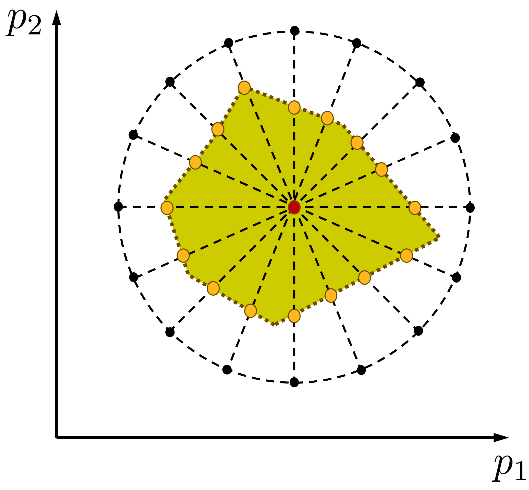
2.5. Radial Line-Search Approach

In assuming interval constrains for each response value $y_i$ according to Equation (21), the corresponding domain of the feasible input parameter domain $\mathbb{A}$ is defined as

$$\mathbb{A}=\left\{{\mathbf{p}}_A\right|y_i^l\le y_i\left({\mathbf{p}}_A\right)\le y_i^u\forall 1\le i\le n\}.$$

(23)

This domain of feasible parameter sets ${\mathbf{p}}_A$ could be analyzed in the case of two input parameters with a line-search approach as illustrated in Figure 3: starting from the optimal parameter set ${\mathbf{p}}_{opt}\in \mathbb{A}$, we search in every direction for the maximum radius of the feasible parameter domain

$${\mathbf{p}}_l=r_l·{\mathbf{a}}_l+{\mathbf{p}}_{opt},r_l\to max\mathrm{subjected}\mathrm{to}{\mathbf{p}}_l\in \mathbb{A},$$

(24)

where ${\mathbf{a}}_l$ is a direction vector of unit length

$$\parallel {\mathbf{a}}_l\parallel =1.$$

(25)

Direction vectors ${\mathbf{a}}_l$ can be chosen randomly or uniformly distributed, as shown in Figure 3, for two input parameters. For each direction, a line-search is performed in order to obtain the maximum possible radius $r_l$ for this direction. This search can be realized by bisection or other methods. The obtained boundary points ${\mathbf{p}}_l$ result in a uniform discretization of the feasible parameter domain $\mathbb{A}$. This approach is similar to the directional sampling method developed for probability integration in reliability analysis [44,45].

In order to extend this method to more than two input parameters, the search directions ${\mathbf{a}}_l$ have to be discretized on a 3D or higher-dimensional (hyper-) sphere. One very efficient discretization method used to obtain almost equally distributed points on the hyper-sphere are Fekete point sets [46], which are generated using a minimum potential energy criterion

$$\Pi =\sum _{1\le i<j\le n_f}{\parallel {\mathbf{a}}_i-{\mathbf{a}}_j\parallel }^{-2}\to min,$$

(26)

where $n_f$ is the number of points on the unit hyper-sphere. The minimization of the potential energy results in equally distributed point sets and will require a significantly smaller number of model evaluations to obtain a suitable representation of the parameter domain boundary. An efficient optimization procedure to solve Equation (26) was proposed in [46]. Once the initial points are generated, a line-search is performed for each of the search directions ${\mathbf{a}}_l$, like with two dimensions. This search procedure was performed in our study using a simple bisection method [47]. However, since every direction can be evaluated independently, a parallel computation of the required model evaluations is possible. The obtained points on the boundary can be used to visualize a discretized shape of the feasible parameter domain. If more than two or three parameters are investigated, this visualization could be displayed in 2D or 3D subspaces.

3. Results

3.1. Bilinear Elasto-Plasticity Model

As a first example, we investigate a uniaxial bilinear elasto-plasticity model defined as follows:

$$\sigma \left(ϵ\right)=\left\{\begin{array}{cc}E·ϵ& ϵ\le {\displaystyle \frac{E}{{\sigma }_Y}}\\ {\sigma }_Y+H·\left(ϵ-{\displaystyle \frac{{\sigma }_Y}{E}}\right)& ϵ>{\displaystyle \frac{E}{{\sigma }_Y}}\end{array}\right.$$

(27)

where $\sigma \left(ϵ\right)$ is the uniaxial stress depending on the uniaxial strain $ϵ$. The model parameters are Young’s modulus E, the yield stress ${\sigma }_Y$, and the hardening modulus H. Figure 4 shows a reference curve for a selected parameter set $E_{ref}=1000$ N/mm², ${\sigma }_{Y,ref}=4.0$ N/mm², and $H_{ref}=100$ N/mm², which is used in the following investigations.

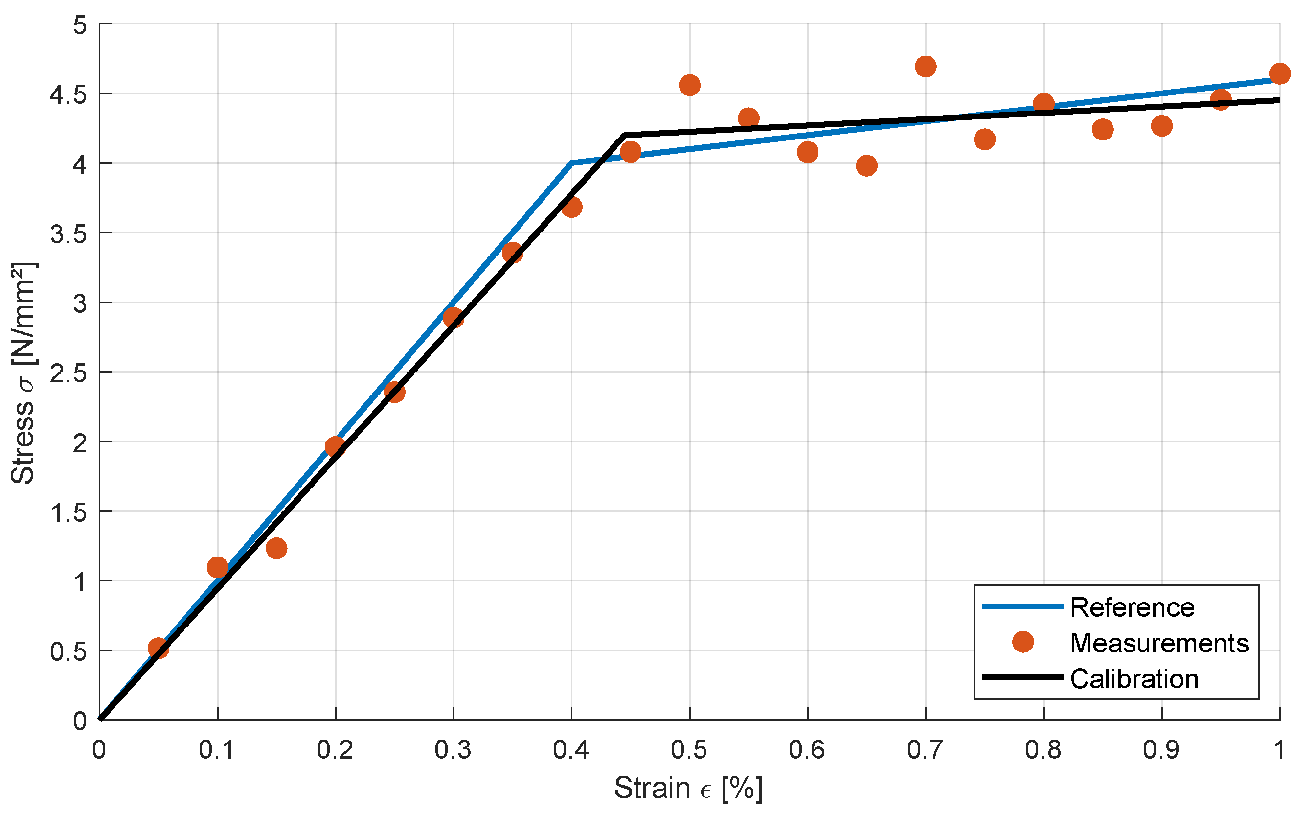
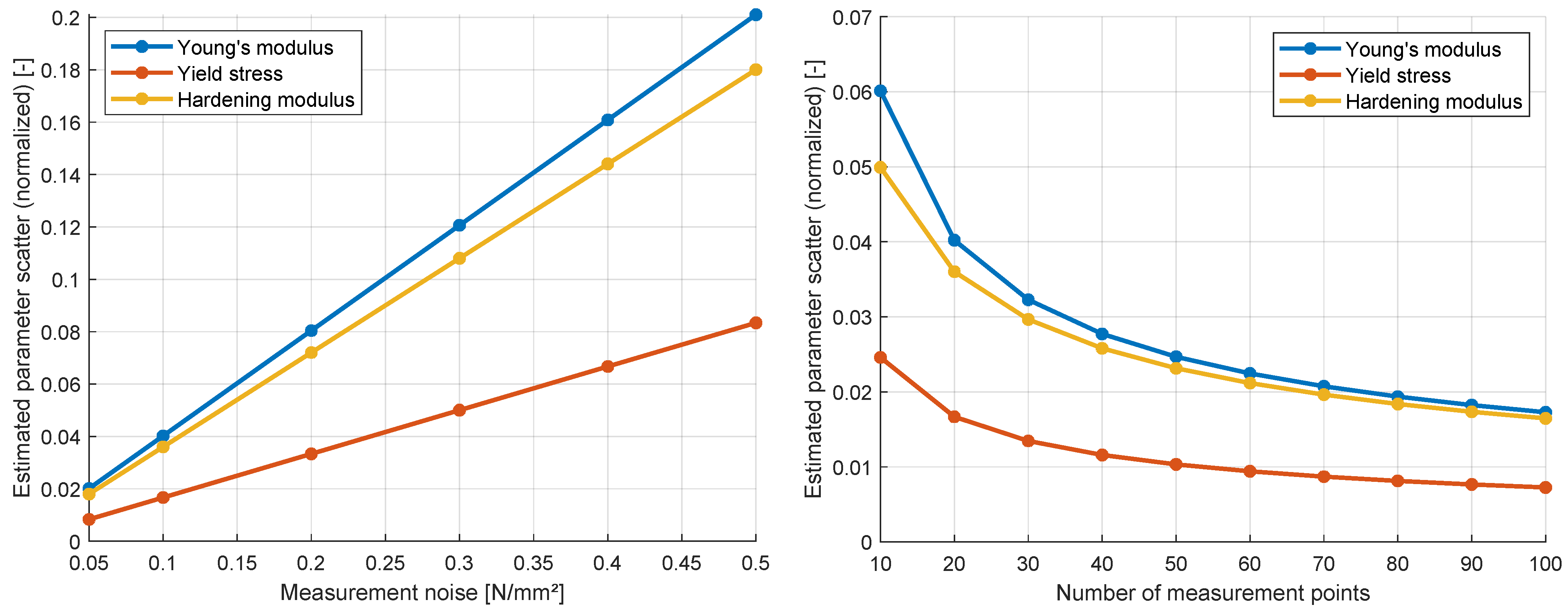
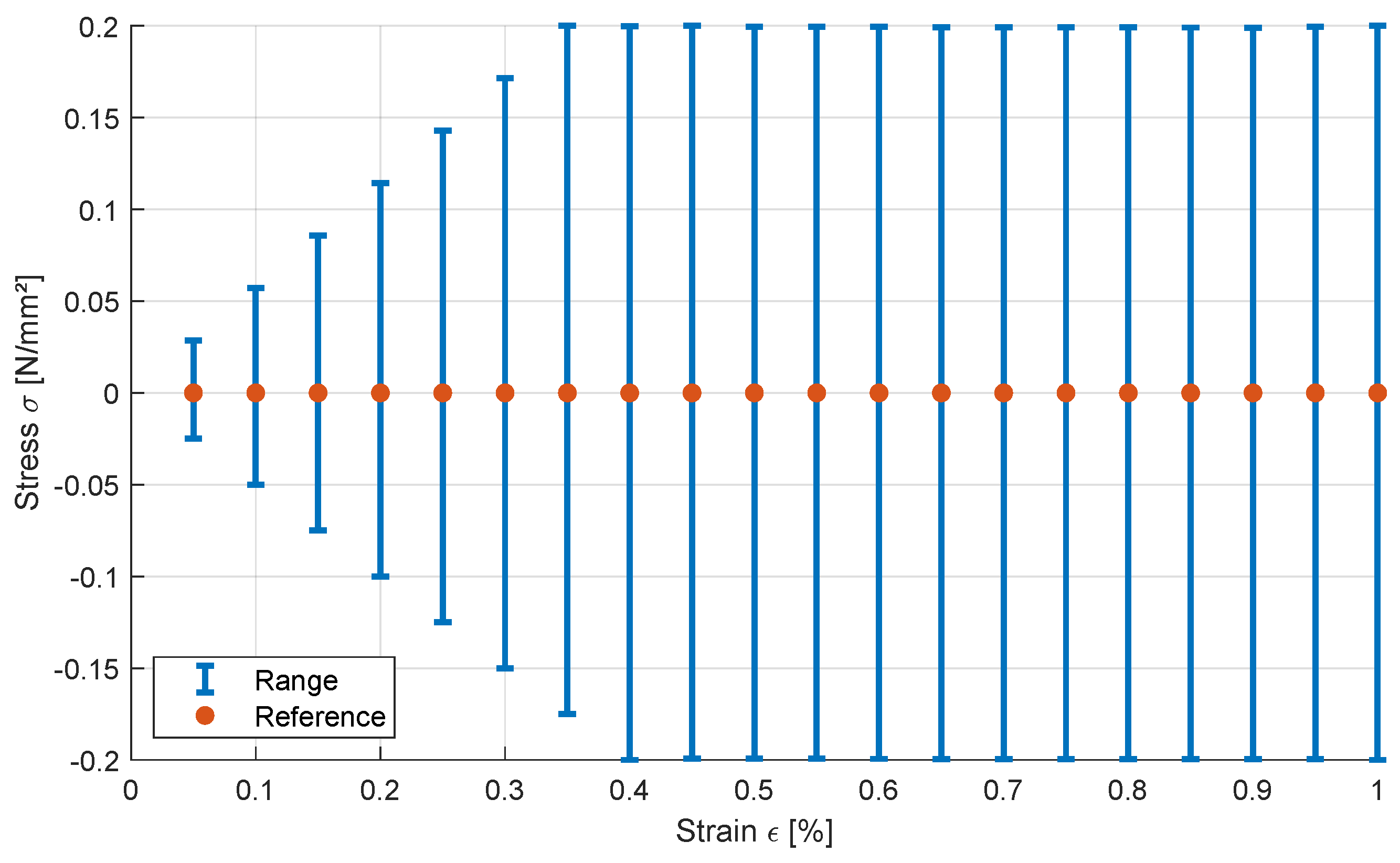
3.1.1. Deterministic Calibration with Noisy Measurements

In assuming additional uncertainties in the measurement points $y_i^{*}$, the obtained optimal parameter set could significantly deviate from the reference parameters, as shown in Figure 4, where an additional Gaussian noise term is used to generate synthetic measurement points

$$y_i^{*}=\sigma ({ϵ}_i,E_{ref},{\sigma }_{Y,ref},{\sigma }_{Y,ref})+\alpha ·\mathcal{N}(0,1),$$

(28)

where $\mathcal{N}(0,1)$ is a normally distributed random number with zero mean and unit variance. If we repeat the calibration of the model with different samples of the noise term, the calibrated optimal parameters will show a certain scatter, which depends on the size of the noise term. In total, 1000 samples of the calibrated parameters are shown as examples in Figure 5 for a noise term of $\alpha =0.1$ N/mm² by considering 20 measurement points, as shown in Figure 4. The figure indicates that all three identified parameters show significant scatter, and the yield stress and the hardening modulus show significant correlation with each other.

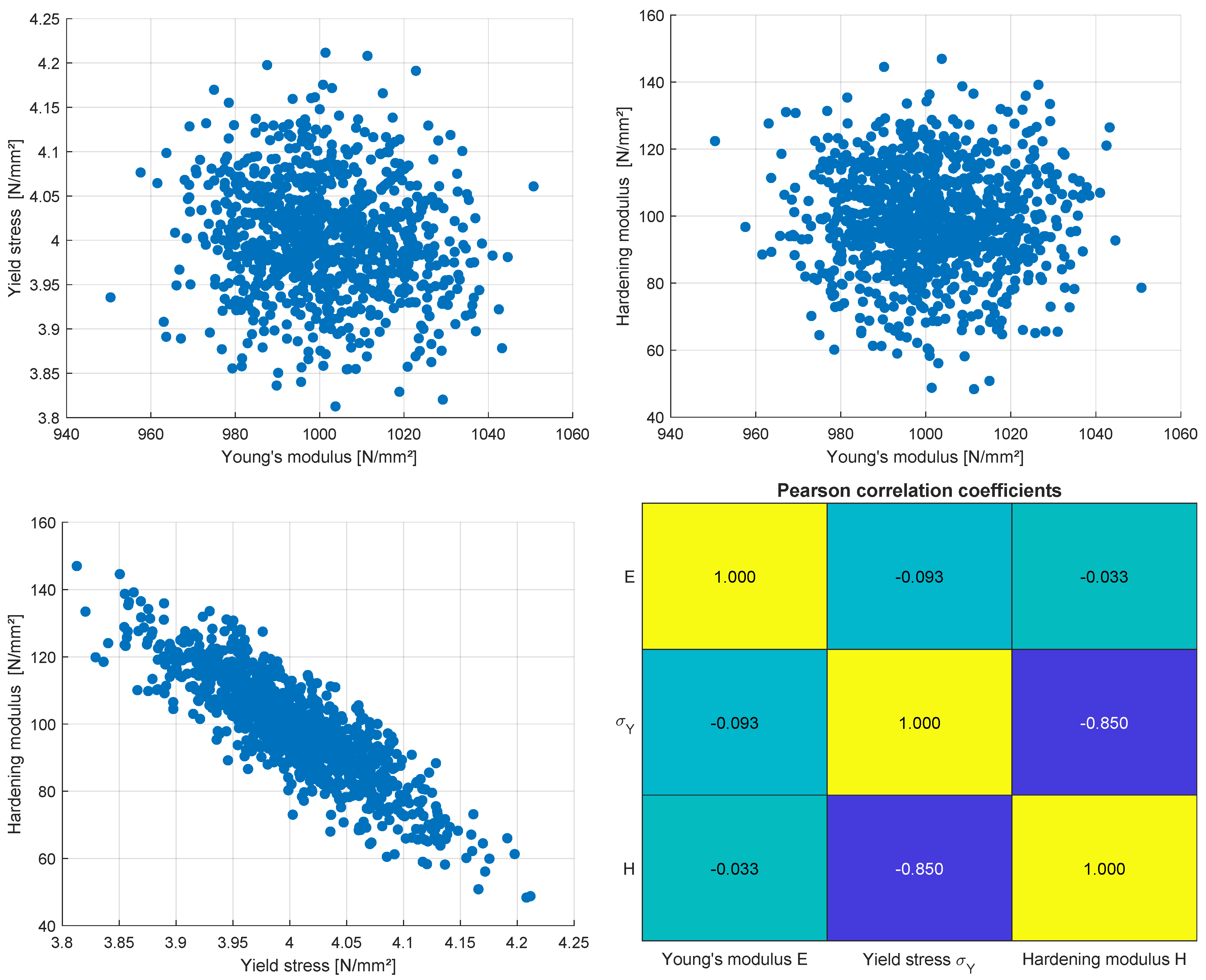
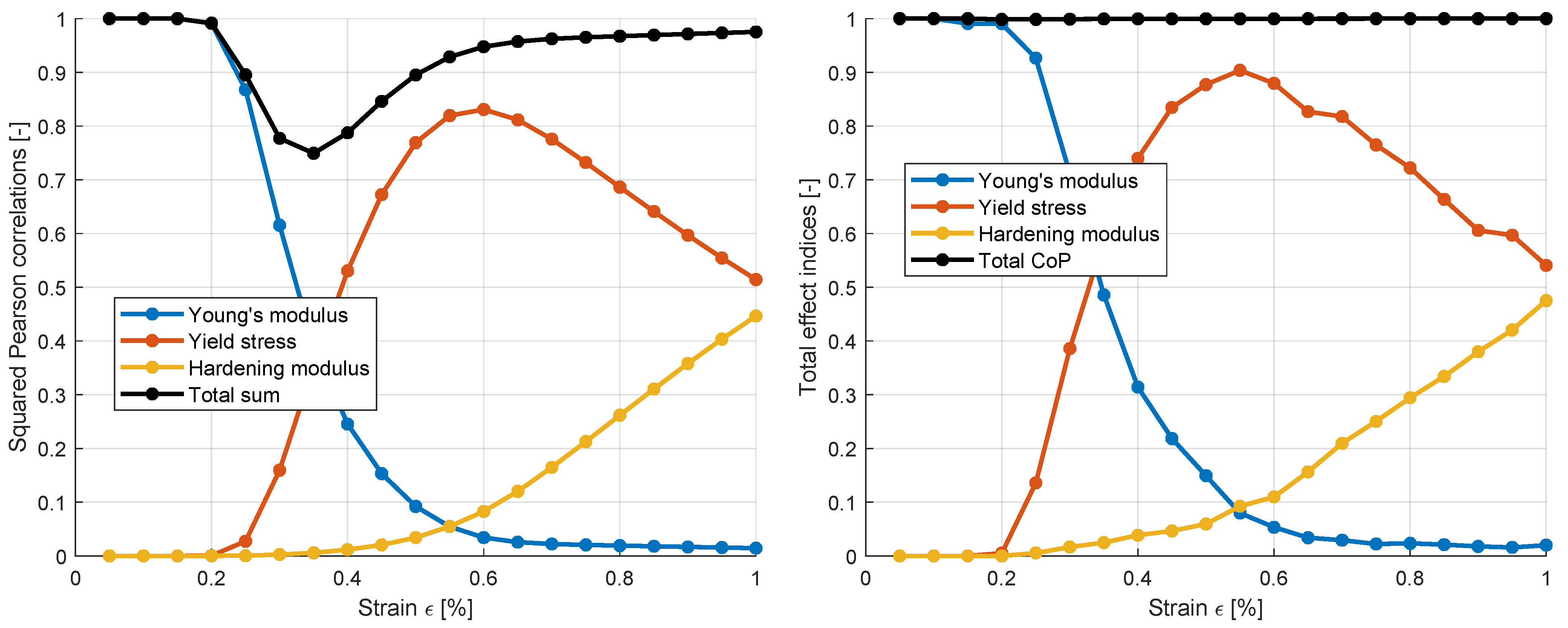
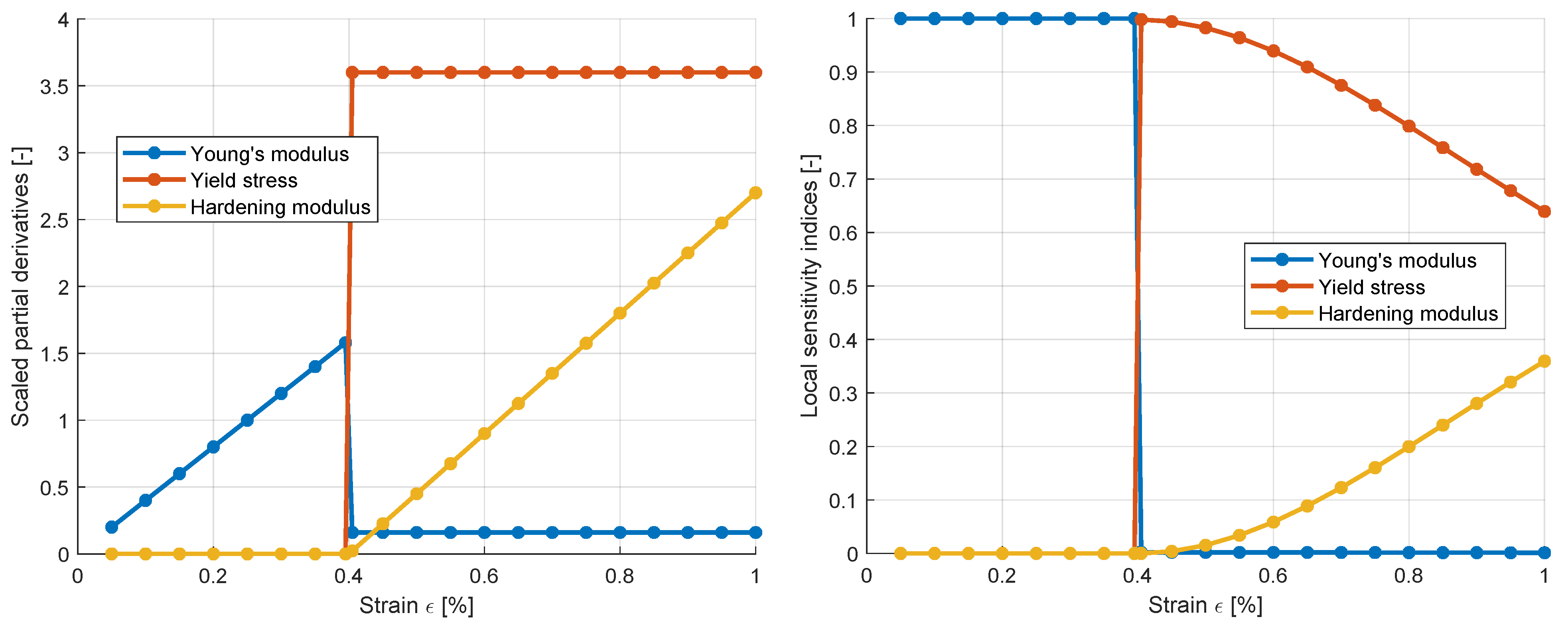
3.1.2. Sensitivity Analysis

By means of the bilinear example, we applied the presented probabilistic approaches and the interval optimization methods. Initially, we performed a sensitivity analysis to investigate the different estimators discussed in Section 2.1. For this purpose, we calculate the sensitivity indices from the squared Pearson correlations by evaluating 20 points on the stress–strain curve. In total, 1000 Latin Hypercube samples were generated by considering the parameter bounds of $E\in [800,1200]$ N/mm², ${\sigma }_Y\in [2.0,6.0]$ N/mm², and $H\in [50,500]$ N/mm². The obtained sensitivity indices shown in Figure 6 indicate that Young’s modulus has a significant influence for smaller strain values, whereas the yield stress and the hardening modulus become more important with increasing strains. However, the sum of the individual sensitivity indices is not close to 1 for strain values between 0.2 and 0.6%, which is caused by the nonlinear relation between these stress values with respect to the model parameters. The sensitivity indices obtained using the MOP approach are evaluated in a second step using the same 1000 samples. As indicated in the figure, these estimates show a similar behavior as the correlation-based estimates. However, the approximation quality of the underlying metamodel is almost excellent for all stress values. Thus, the estimated total effect indices are more reliable measures for judging the sensitivity of the model parameters for this example.

3.1.3. Maximum Likelihood Approach

In the next step, the Markov estimator is applied using Equation (13) to estimate the parameter covariance matrix from the measurement covariance matrix. Again, 20 measurement points are considered on the hardening curve with a constant measurement error of ${\sigma }_y=0.1$ N/mm². The covariance matrix is assembled according to Equation (14). The required sensitivity matrix in Equation (12) is estimated using a central difference at the optimal parameter set, which requires only six additional model evaluations. In Figure 7, the estimated scatter of the parameters is visualized by generating 1000 samples of the estimated parameter covariances. The figure indicates a similar scatter and correlation for the parameters as those obtained with the 1000 calibration runs shown in Figure 5. Figure 8 shows the normalized derivatives of the sensitivity matrix.

In the next step, the influence of the assumed measurement error ${\sigma }_y$ and the number of measurement points $y_i$ is investigated. Figure 9 shows the estimated parameter scatter normalized with the parameter ranges depending on the size of an independent measurement error according to Equation (14) for 20 measurement points. The figure indicates a linear relation of the standard deviation for all three parameters, as expected from the formulation in Equation (15). The normalized parameter scatter of the yield stress is significantly smaller compared to the scatter of Young’s and hardening moduli. This is caused by the fact that the sensitivity of the yield stress is on average larger, as observed in the normalized partial derivatives in Figure 8. Additionally, the influence of the number of measurement points is shown in Figure 9 for a constant ${\sigma }_y=0.1$ N/mm². This figure clearly indicates that with an increasing number of independent measurement points, the estimated scatter and, thus, the uncertainty decreases. This problem is investigated in detail in [48] and could be resolved only if a realistic correlation between the measurement points is assumed in the covariance matrix.

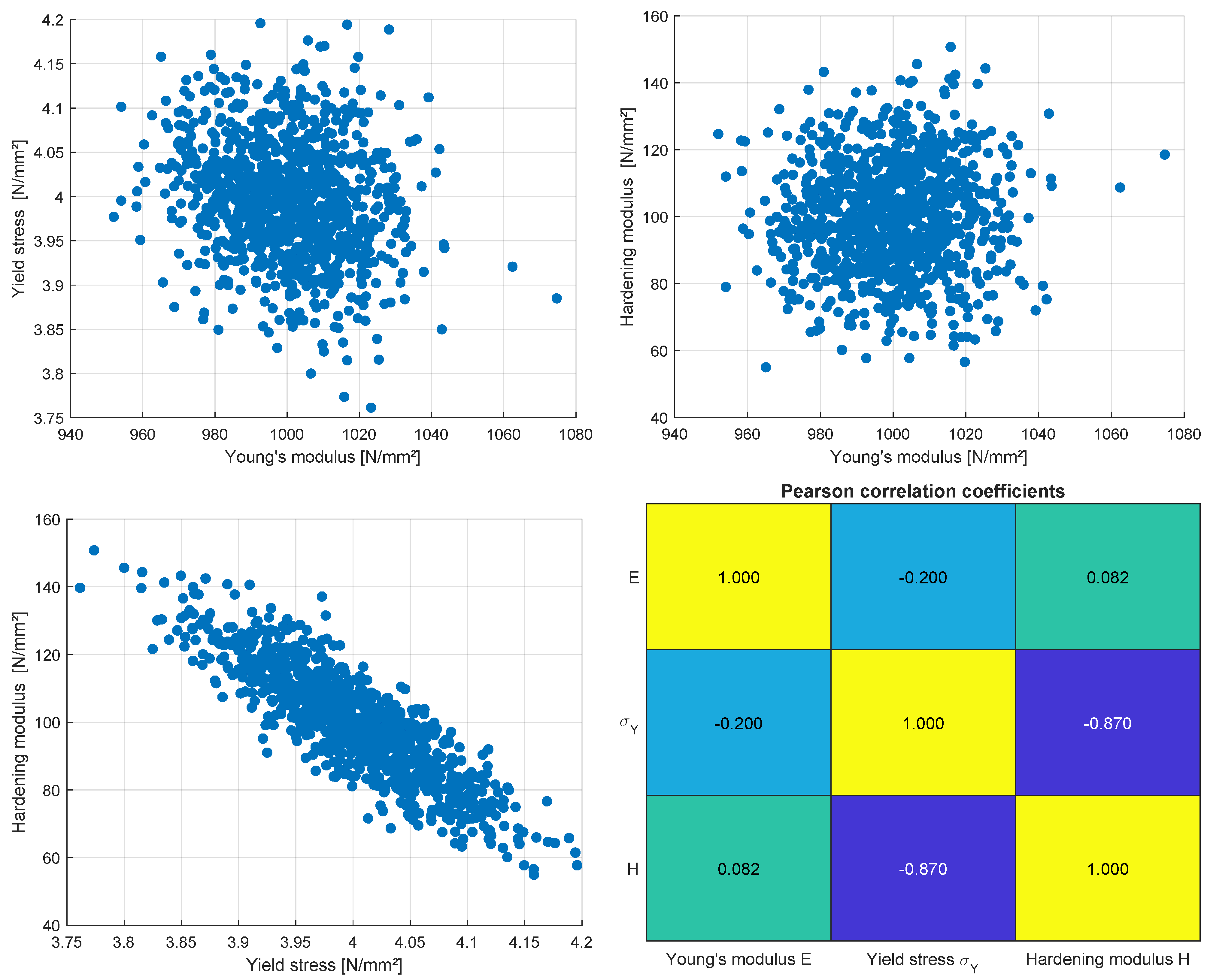
3.1.4. Bayesian Updating

The Bayesian updating approach is investigated next using a constant measurement error ${\sigma }_y=0.1$ N/mm² and a diagonal covariance matrix as in the previous investigations with a Markov estimator. The posterior distribution in Equation (19) is evaluated for the bilinear model using the Metropolis–Hastings algorithm with 20,000 samples, whereby the first 2000 samples of the so-called burn-in phase are neglected in the statistical analysis. In Figure 10, the estimated parameter scatter is shown. The pair-wise anthill plots and the correlation matrix indicate good agreement with the results of the Markov estimator shown in Figure 7. This may be explained by the approximately linear behavior of the model for small parameter variations.

In Figure 11, the estimated mean values and the variation in the model response values are visualized for the generated samples. The figure indicates good agreement with the mean response values with the deterministic reference curve. Around a deterministic yield strain of $0.4\%$, a larger deviation could be observed. More interesting is the standard deviation of the individual stress responses. In contrast to the assumption of a constant measurement error of ${\sigma }_y=0.1$ N/mm², the variation in all stress values is smaller, caused by the inherent correlations of the model responses.

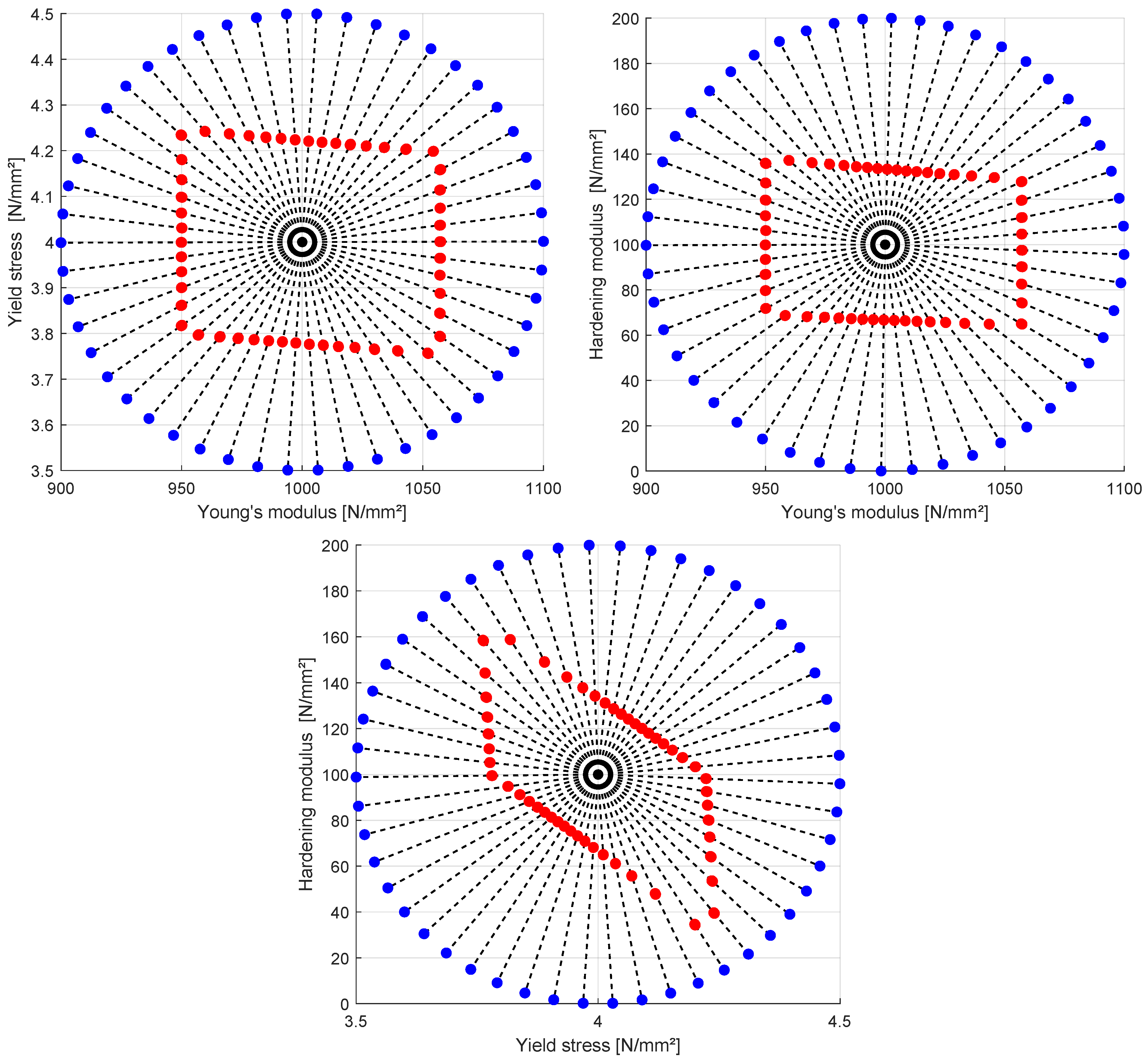
3.1.5. Interval Optimization and Radial Line-Search

Next, the presented interval approaches are applied for the bilinear model by considering a constant measurement interval size of $\Delta y_i=\pm 0.2$ N/mm². First, the minimum and maximum parameter values are obtained with two optimization runs for each model parameter using an evolutionary algorithm from the Ansys optiSLang software package [41] with 25 generations and a population size of 20. The obtained best parameter sets of each optimization run are shown in Figure 12, which span a three-dimensional box around the reference parameter set.

Figure 10. Bilinear model: estimated parameter scatter using Bayesian updating with 20 measurement points on the stress–strain curve and independent measurement errors ${\sigma }_y=0.1$ N/mm².

Figure 10. Bilinear model: estimated parameter scatter using Bayesian updating with 20 measurement points on the stress–strain curve and independent measurement errors ${\sigma }_y=0.1$ N/mm².

Figure 11. Bilinear model: estimated response statistics of Bayesian parameter samples assuming independent measurement errors with ${\sigma }_y=0.1$ N/mm².

Figure 11. Bilinear model: estimated response statistics of Bayesian parameter samples assuming independent measurement errors with ${\sigma }_y=0.1$ N/mm².

Figure 12. Bilinear model: obtained parameter sets for the minimization and maximization of Young’s modulus (blue), the yield stress (red), and the hardening modulus (green) considering a measurement interval of $\Delta y_i=\pm 0.2$ N/mm².

Figure 12. Bilinear model: obtained parameter sets for the minimization and maximization of Young’s modulus (blue), the yield stress (red), and the hardening modulus (green) considering a measurement interval of $\Delta y_i=\pm 0.2$ N/mm².

Second, the radial line-search approach is applied for different 2D subspaces by considering two model parameters as optimization variables, while the third is kept at the reference value. In Figure 13, the initial radial search points and the finally obtained boundary points are shown for all 2D subspaces. The initial parameter bounds were chosen from the previous optimization results as $E\in [900,1100]$ N/mm², ${\sigma }_Y\in [3.5,4.5]$ N/mm², and $E\in [0,200]$ N/mm², and 50 uniformly distributed search directions are considered for each subspace. The subspace plots in Figure 13 indicate an almost rectangular boundary of the feasible Young’s modulus–yield stress subspace and Young’s modulus–hardening modulus subspace; meanwhile, in the third subspace, the yield stress–hardening modulus subspace, the boundary indicates a significant dependence on the feasible parameter values.

Finally, the bilinear example is investigated with the radial line-search with all three parameters. For this purpose, 500 uniformly distributed Fekete points are generated on the unit sphere by considering the parameter bounds of the 2D analysis. The line-search is performed for each direction individually with a bisection with 10 refinement steps. In Figure 14, the initial search points are shown together with the obtained boundary points for all 500 directions. In the figure, a Delaunay triangulation of the convex hull of boundary points is used for better visualization purposes utilizing the MATLAB plotting library [49]. The obtained feasible parameter domain indicates a dependence between the yield stress and hardening modulus similar to in the 2D analyses. The ranges of the response values of the obtained boundary points are given in Figure 15, where most values approach the $\pm 0.2$ N/mm² interval. For strain values below $0.4\%$, the maximum and minimum response values decrease linearly due to the pure elastic behavior and the resulting perfect correlation of the stress–strain curves.

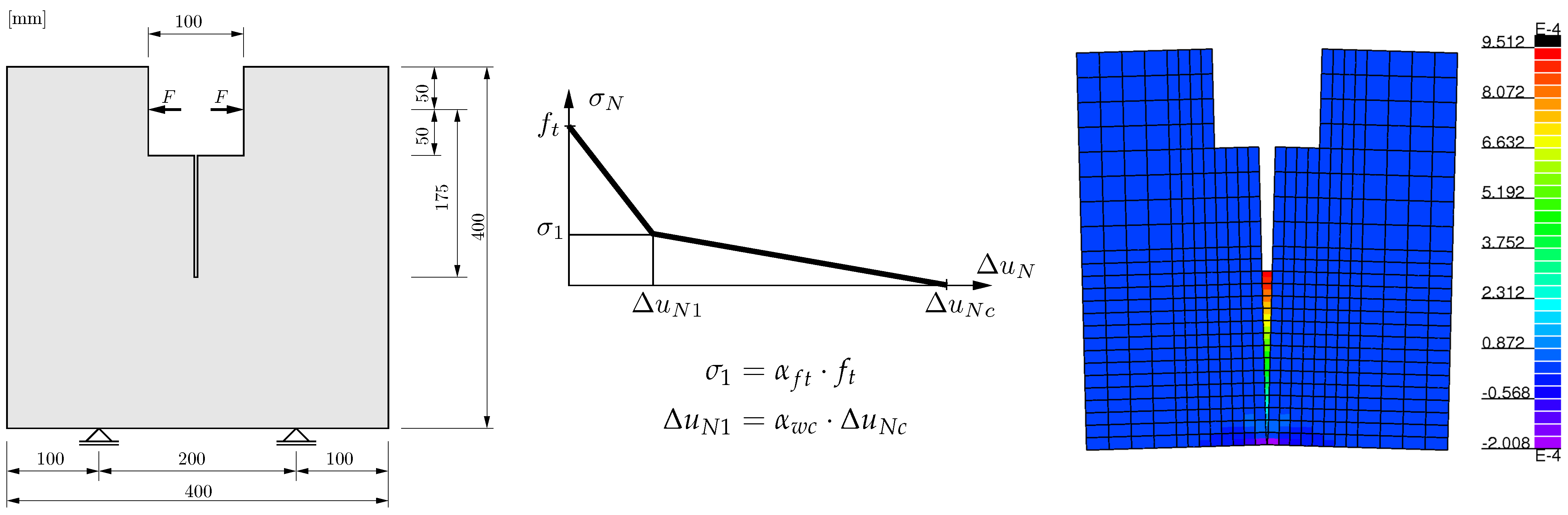
3.2. Tension-Softening Model for Concrete Cracking

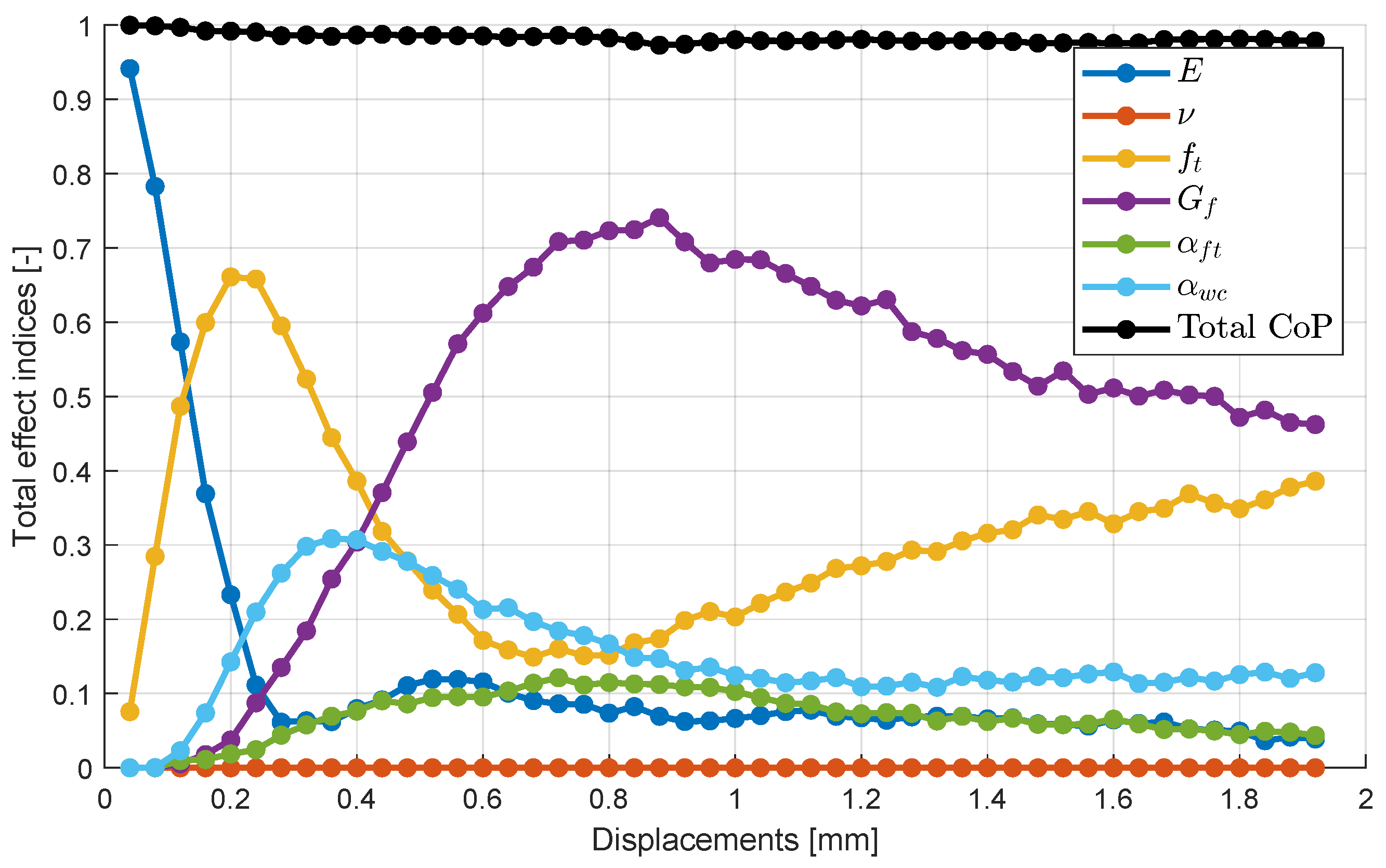
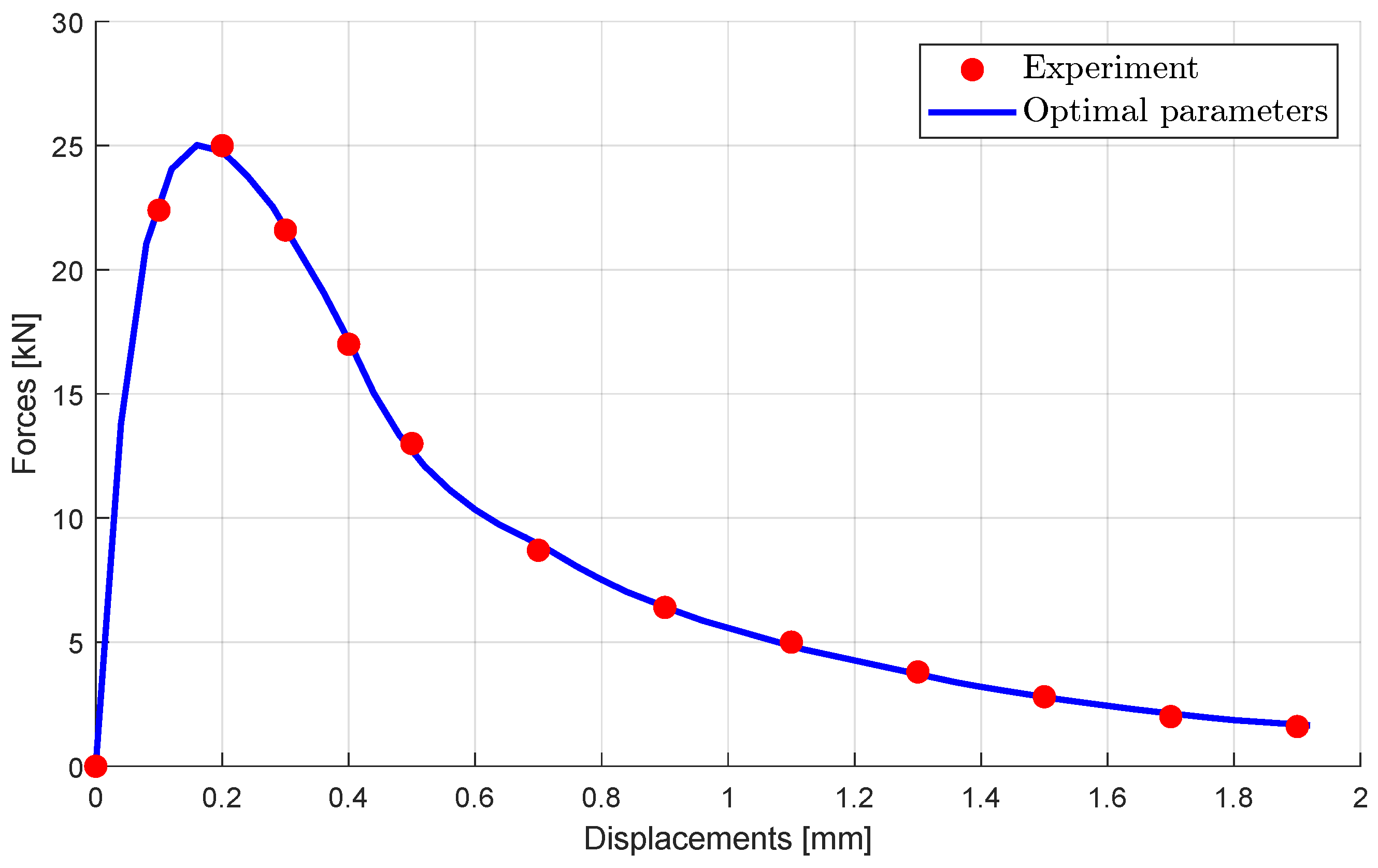
3.2.1. Sensitivity Analysis and Deterministic Parameter Optimization

By means of the second numerical example, the material parameters of plain concrete are identified using the measurement results of a wedge splitting test, published in [50]. The geometry of the investigated concrete specimen is shown in Figure 16. The softening curve is obtained by displacement-controlled simulation. The simulation model was discretized with 2D finite elements and considered an elastic base material and a predefined crack with a bilinear softening law. The displacements were measured as the relative displacements between the load application points. Further details about the simulation model can be found in [51].

Six unknown parameters are identified with the presented methods: Young’s modulus E, Poisson’s ratio $\nu$, the tensile strength $f_t$, the Mode-I fracture energy $G_f$, and two shape parameters ${\alpha }_{ft}$ and ${\alpha }_{wc}$, which define the kink of the bilinear softening law in terms of the tensile stress ${\sigma }_1={\alpha }_{ft}·f_t$ and the relative displacements normal to the crack surface $\Delta u_{N1}={\alpha }_{wc}·\Delta u_{Nc}$. In

Table 1. Wedge splitting test: initial material parameter bounds and optimal values.

Parameter	Unit	Reference Value	Bounds	Deterministic Optimization
Young’s modulus E	${10}^{10}$ N/m2	2.830	1.00–6.00	4.176
Poisson’s ratio $\nu$	−	0.180	0.10–0.40	-
Tensile strength $f_t$	${10}^6$ N/m2	2.270	1.00–4.00	2.003
Fracture energy $G_f$	${10}^2$ N/m2	2.850	2.00–4.00	2.850
Shape parameter ${\alpha }_{ft}$	−	0.163	0.05–0.50	0.150
Shape parameter ${\alpha }_{wc}$	−	0.242	0.05–0.50	0.258

, the reference parameters according to [50] and the defined parameter bounds for the calibration are given.

As a first step, the sensitivity of the material parameters with respect to the simulated force values was investigated by generating 200 samples within the defined bounds using improved Latin Hypercube sampling according to [43]. The corresponding force–displacement curves of these samples are given in Figure 17 in addition to the experimental values according to [50]. The total effect sensitivity indices of the model parameters are estimated for each force value on the load–displacement curve using the Metamodel of Optimal Prognosis [35] approach, as discussed in Section 2.1. These sensitivity indices are shown in Figure 18 depending on the displacement values. The figure indicates that Poisson’ ratio is not sensitive to any of the simulation results. Because of this finding, we do not consider it in the following parameter calibration and uncertainty estimation. The other parameters show a certain influence whereby Young’s modulus, the tensile strength, and the fracture energy are most important.

The optimal parameter set is determined by least squares minimization using Equation (1), whereby the deviation in the response values is evaluated at the 13 displacement values of the experimental measurement points. As an optimization approach, the Adaptive Response Surface Method of the Ansys optiSLang software package [41] was utilized, which required 220 model evaluations. The obtained optimal parameter values are given in Table 1, and the corresponding load–displacement curve is shown in Figure 19, which indicates almost perfect agreement with the experimental values.

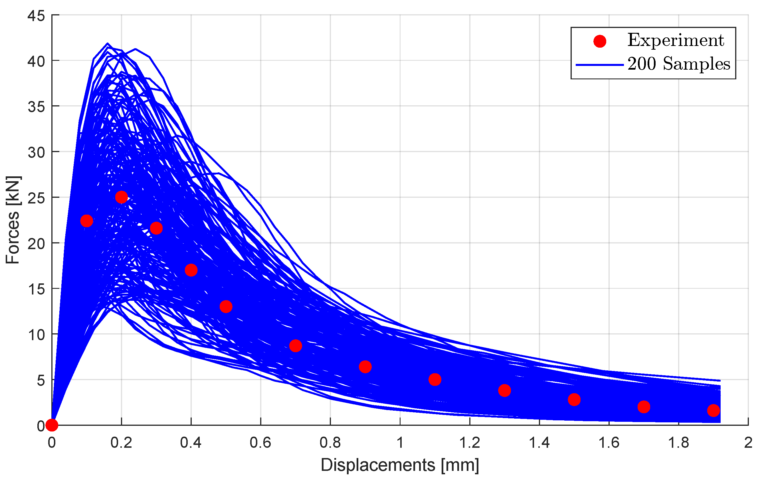
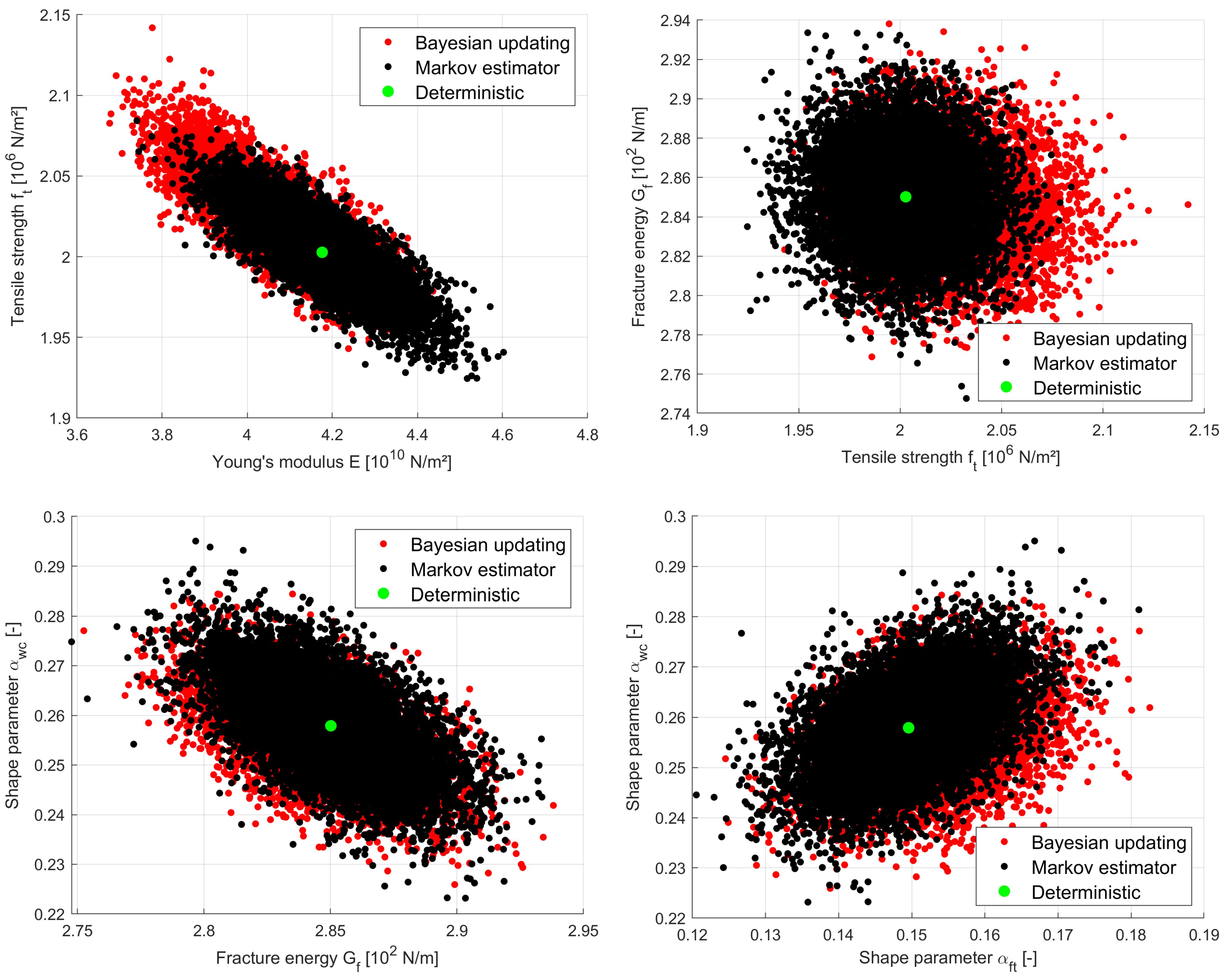
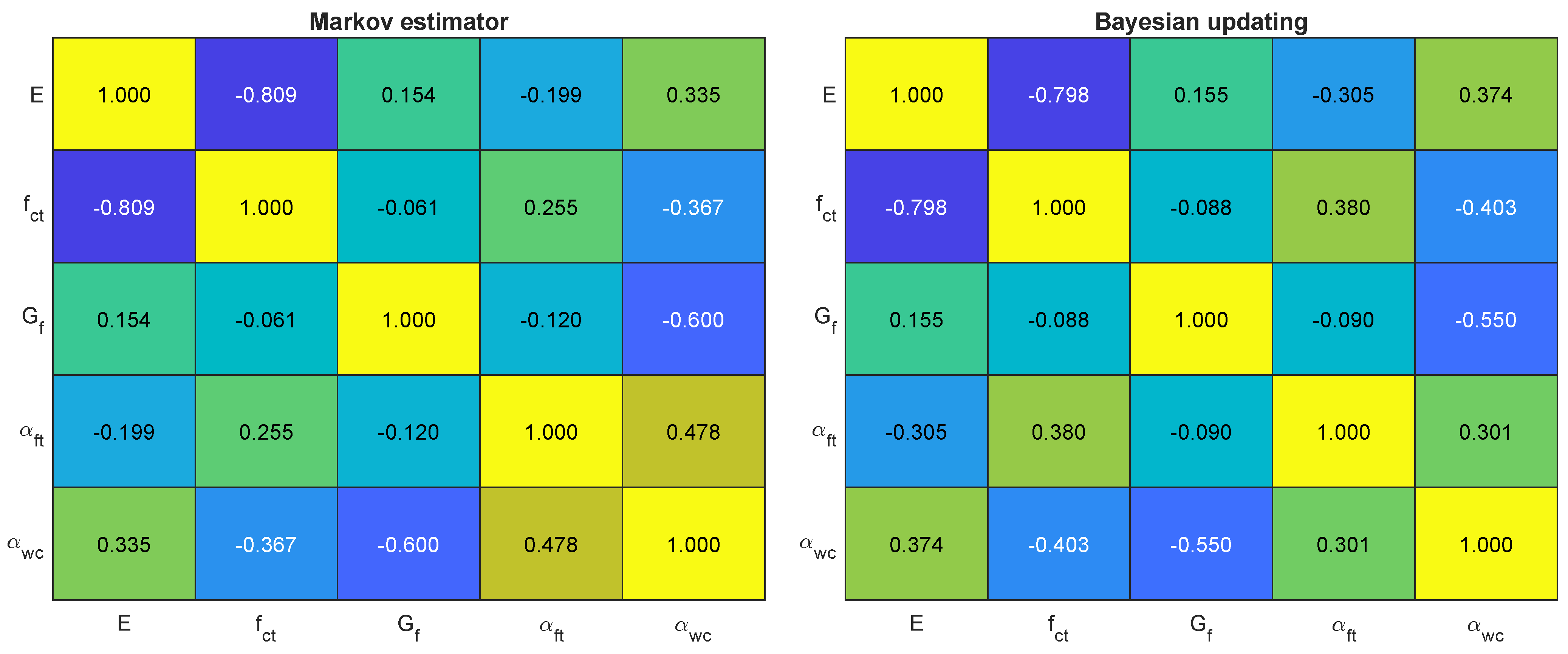
3.2.2. Probabilistic Uncertainty Estimation

In the next step, the Markov estimator and the Bayesian updating approaches are applied to estimate the parameter uncertainties. The covariance matrix of the 13 measurement points are defined according to Equation (14) as a diagonal matrix, whereby a constant standard deviation is assumed as the root mean squared error of the deterministic calibration as

$${\sigma }_y=\sqrt{{\displaystyle \frac{1}{n}}\sum _{i=1}^n{(y_i-y_i^{*})}^2}=151.4\mathrm{N}.$$

The parameter uncertainty values estimated using the Markov estimator are given in

Table 2. Wedge splitting test: estimated statistical properties of the identified parameters using the Markov estimator and Bayesian updating.

Parameter		Unit	Markov Estimator			Bayesian Updating
			Mean	Stddev	CoV	Mean	Stddev	CoV
Young’s modulus E		${10}^{10}$ N/m2	4.176	0.116	0.028	4.065	0.136	0.033
Tensile strength $f_t$		${10}^6$ N/m2	2.003	0.023	0.011	2.025	0.030	0.015
Fracture energy $G_f$		${10}^2$ N/m	2.850	0.024	0.008	2.847	0.026	0.009
Shape parameter ${\alpha }_{ft}$		−	0.150	0.008	0.051	0.153	0.008	0.055
Shape parameter ${\alpha }_{wc}$		−	0.258	0.009	0.034	0.256	0.009	0.035

. The mean values are the optimal parameter values from the previous deterministic optimization. The standard deviation and the parameter correlation matrix are obtained from the estimated covariance matrix using Equation (15). The partial derivatives required in Equation (12) are estimated using a central differences approach with an interval of $0.01\%$ of the initial parameter ranges. Thus, only 10 additional model evaluations were necessary to apply the Markov estimator for this example.

The results in Table 2 indicate that the shape parameters and Young’s modulus have a significantly larger coefficient of variation (CoV) compared to the tensile strength and the fracture energy. This can be explained if we compare the sensitivity indices of the parameters given in Figure 18, where the fracture energy and the tensile strength have, on average, the largest values. The estimated parameter correlation matrix is given in Figure 20, which indicates a significant correlation between Young’s modulus and the tensile strength. Further dependencies could be observed between the fracture energy and one of the shape parameters. Additionally, the figure shows some interesting pair-wise anthill plots with 10,000 samples generated with the multivariate normal distribution considering the estimated parameter covariance matrix of the Markov estimator.

Next, Bayesian updating is performed with the same diagonal measurement covariance matrix used for the Markov estimator. In total, 50,000 samples are generated with the Metropolis–Hastings algorithm, whereby 5000 samples of the burn-in phase are neglected in the statistical analysis. The remaining 45,000 samples are shown in Figure 20. In Table 2, the corresponding statistical estimates are given. The table and the pair-wise anthill plots indicate that the mean values differ significantly from the Markov estimator results for Young’s modulus and the tensile strength. Good agreement of the statistical properties is obtained for the fracture energy and the shape parameters. Even the estimated parameter correlations are quite close to the Markov estimator results.

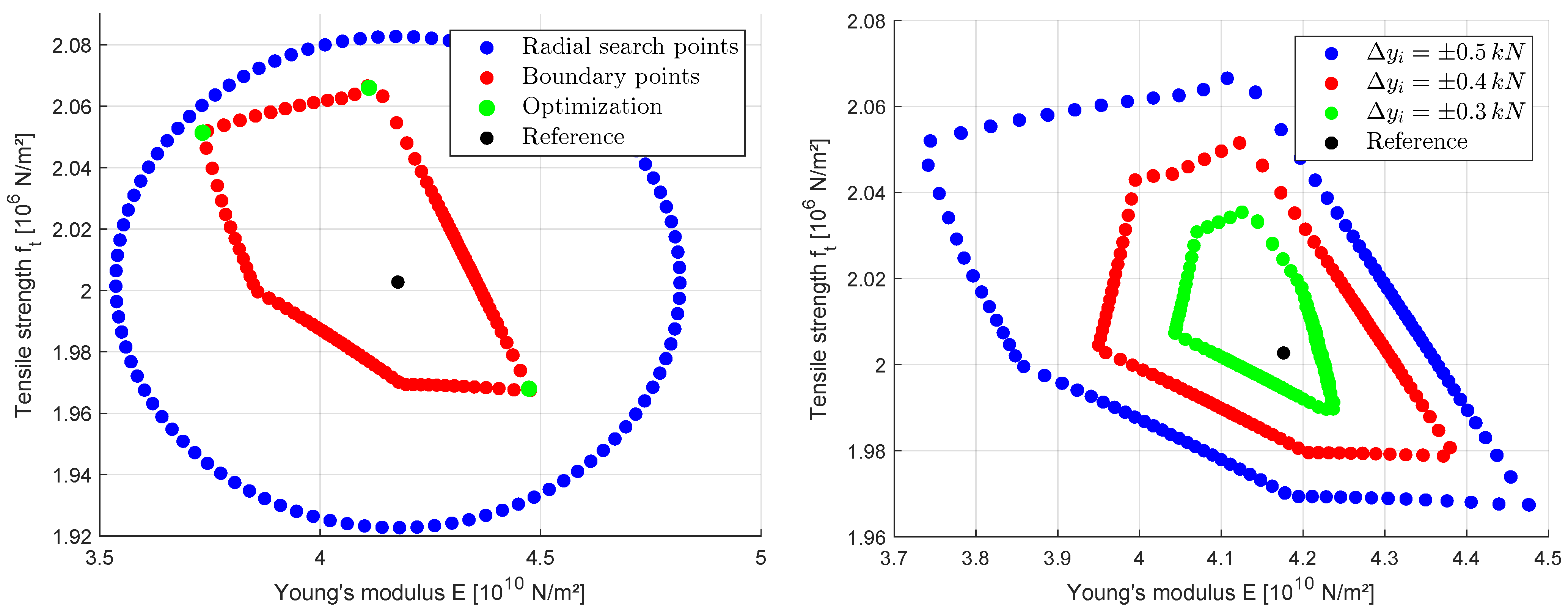
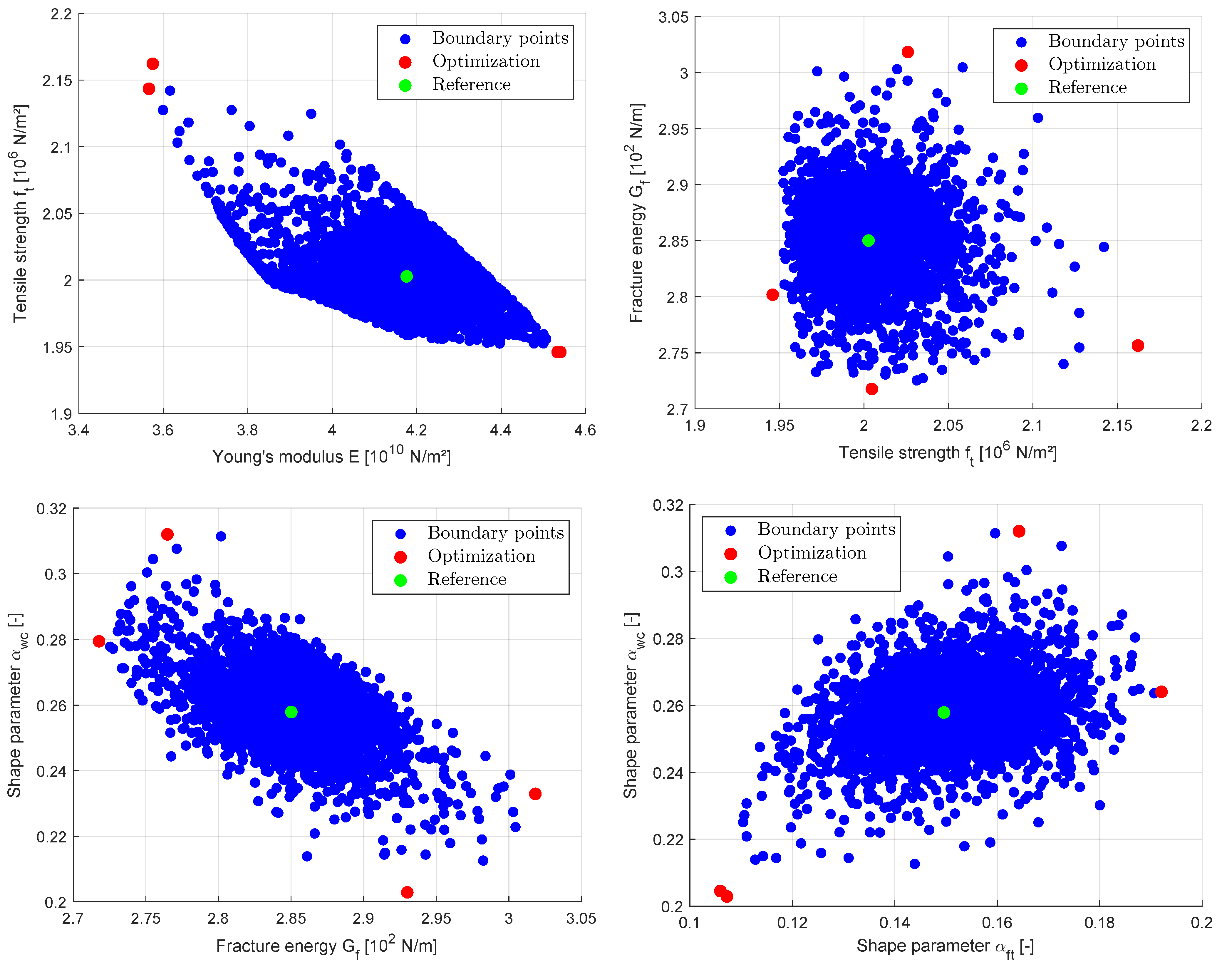
3.2.3. Interval Approaches

Finally, the proposed radial line-search algorithm is demonstrated by means of this example. As a first step, only Young’s modulus and the tensile strength are considered uncertain parameters; meanwhile, the remaining parameters are kept constant. The resulting two-dimensional search points are shown in Figure 21 for an assumed measurement interval of $\Delta y_i=\pm 0.5$ kN, which corresponds to 3.3 times the RMSE. This interval is equivalent to the $99.9\%$ confidence interval of the previously assumed measurement uncertainty. The figure clearly indicates that the feasible 2D parameter domain is non-symmetric and bounded by different linear and nonlinear segments. Different $\alpha$-levels could be investigated if the measurement interval is modified in the analysis. Figure 21 also shows the domain boundary for different values of $\Delta y_i$, where a nonlinear shrinkage of the domain boundary could be observed. The figure clearly indicates that the obtained parameter domain boundary is not symmetric, as assumed by the Markov estimator.

In a second step, all five sensitive parameters are considered in the radial line-search. A total of 5000 directions were investigated in this analysis, where the ranges of the hyper-sphere are given in

Table 3. Wedge splitting test: parameter bounds in the 5D parameter space obtained with the interval optimization and defined ranges for the radial line-search approach.

Parameter		Unit	Reference	Optimization		Line-Search Ranges
				Min	Max
Young’s modulus E		${10}^{10}$ N/m2	4.176	3.566	4.540	±1.200
Tensile strength $f_t$		${10}^6$ N/m2	2.003	1.946	2.162	±0.176
Fracture energy $G_f$		${10}^2$ N/m2	2.850	2.718	3.018	±0.240
Shape parameter ${\alpha }_{ft}$		−	0.150	0.106	0.192	±0.080
Shape parameter ${\alpha }_{wc}$		−	0.258	0.203	0.312	±0.080

. The table also shows the minimum and maximum possible parameters bounds obtained with the interval optimization approach by assuming the measurement interval to be $\Delta y_i=\pm 0.5$ kN. For each minimization and maximization task, again, the evolutionary algorithm from the Ansys optiSLang software package [41] with 25 generations and a population size of 20 was applied. The minimum and maximum parameter values are shown together with the obtained 5000 boundary points of the radial line-search approach in Figure 22 for some selected parameter subspaces. The figure indicates a non-symmetric dependence for Young’s modulus and the tensile strength. The dependence between the other parameters seems to be similar to the results obtained with Bayesian updating.

Since the evaluation of the radial line search requires a huge number of model evaluations, we will investigate the accuracy of different approximation methods by means of this example. First, a linear approximation model from the 10 samples of the central differences approach within an interval of $\pm 0.05\%$ of the initial parameter ranges is investigated. We apply the radial line-search on this 5D approximation model as investigated previously only in the 2D subspace with Young’s modulus and the tensile strength as uncertain parameters; meanwhile, the remaining parameters are kept constant. In Figure 23, the results obtained using the original FEM model are compared to results obtained with the linear approximation model. The figure indicates an already sufficient accuracy, which represents the main characteristics of the feasible parameter domain. The 2D analysis was chosen to enable a more clear visualization of the approximation errors.

Additionally, we applied a full quadratic approximation model based on 100 Latin Hypercube samples generated within the $\pm 0.05\%$ domain of all five parameters around the optimal parameter values ${\mathbf{p}}_{opt}$. The results of the 2D line-search shown in Figure 23 are quite similar to those obtained with the linear model, but still show a certain deviation from the FEM solutions. In order to obtain a better representation of the nonlinear dependencies of the model responses and the model parameters in the range of the parameter scatter, we apply the Metamodel of Optimal Prognosis as a more sophisticated surrogate to the response values obtained from the 100 LHS samples within the $\pm 0.05\%$ parameter ranges. As indicated additionally in Figure 23, the straightforward application of the MOP already yields quite accurate results. An additional improvement of the surrogate model could be achieved by considering the obtained 100 boundary points of the line-search procedure as additional support points within the surrogate model, which results in an almost perfect agreement with the line-search results.

4. Conclusions

In this study, we investigated well-known probabilistic approaches as benchmark methods for the uncertainty quantification of calibrated material parameters. The applied Markov estimator and Bayesian updating require knowledge of the measurement covariances to estimate the multivariate probability density function of the calibrated model parameters. Often, this matrix can be estimated quite roughly based on a few measurement curves. If the covariance matrix is assumed as a diagonal matrix, this implies independent measurement errors and the estimated scatter parameter directly depends on the number of considered points on the measurement curve. As a consequence, the obtained results might be difficult to interpret, and a successful application of the probabilistic approaches would require a more accurate estimate of the measurement covariance matrix.

In order to overcome this limitation, an interval optimization approach which assumes only the maximum and minimum values of the measurement points was extended in this study. With th ehelp of this approach, the full feasible parameter domain fulfilling the defined measurement intervals could be determined through a novel radial line-search procedure, which searches for the boundary of the feasible parameter space based on the underlying simulation model. The boundary domain is discretized with uniformly distributed Fekete points that define the radial directions based on the optimal parameter set obtained in the previous deterministic calibration. For each direction, the boundary point was obtained with a one-dimensional line-search procedure. Compared to previous interval search procedures, such as those published in [26,30,31], the presented approach does not require any assumption on the parameter correlation.

However, the computation requires numerous model evaluations but can be computed in parallel for each independent search direction. The computational burden could be reduced significantly using either low-order approximation schemes or by applying more sophisticated surrogate models on support points around the optimal parameter set. This is an area for further research to determine a fully automatic adaptive scheme based on surrogate models.

As a result of the presented approach, we obtained the boundary of the feasible parameter domain by means of a given number of discretization points in the parameter input space. The transfer to a closed description of the parameter uncertainty, e.g., with correlated interval numbers, is an open question that should motivate further research.

References

1. Beck, J.V.; Arnold, K.J. Parameter Estimation in Engineering and Science; Wiley Interscience: New York, NY, USA, 1977. [Google Scholar]
2. Most, T. Identification of the parameters of complex constitutive models: Least squares minimization vs. Bayesian updating. In Proceedings of the 15th Working Conference IFIP Working Group 7.5 on Reliability and Optimization of Structural Systems, Munich, Germany, 7–10 April 2010. [Google Scholar]
3. Ereiz, S.; Duvnjak, I.; Fernando Jiménez-Alonso, J. Review of finite element model updating methods for structural applications. Structures 2022, 41, 684–723. [Google Scholar] [CrossRef]
4. Machaček, J.; Staubach, P.; Tavera, C.E.G.; Wichtmann, T.; Zachert, H. On the automatic parameter calibration of a hypoplastic soil model. Acta Geotech. 2022, 17, 5253–5273. [Google Scholar] [CrossRef]
5. Scholz, B. Application of a Micropolar Model to the Localization Phenomena in Granular Materials: General Model, Sensitivity Analysis and Parameter Optimization. Ph.D. Thesis, Universität Stuttgart, Stuttgart, Germany, 2007. [Google Scholar]
6. Simoen, E.; De Roeck, G.; Lombaert, G. Dealing with uncertainty in model updating for damage assessment: A review. Mech. Syst. Signal Process. 2015, 56, 123–149. [Google Scholar] [CrossRef]
7. Ledesma, A.; Gens, A.; Alonso, E. Estimation of parameters in geotechnical backanalysis—I. Maximum likelihood approach. Comput. Geotech. 1996, 18, 1–27. [Google Scholar] [CrossRef]
8. Rappel, H.; Beex, L.A.; Noels, L.; Bordas, S. Identifying elastoplastic parameters with Bayes’ theorem considering output error, input error and model uncertainty. Probabilistic Eng. Mech. 2019, 55, 28–41. [Google Scholar] [CrossRef]
9. Rappel, H.; Beex, L.A.; Hale, J.S.; Noels, L.; Bordas, S. A tutorial on Bayesian inference to identify material parameters in solid mechanics. Arch. Comput. Methods Eng. 2020, 27, 361–385. [Google Scholar] [CrossRef]
10. Bi, S.; Beer, M.; Cogan, S.; Mottershead, J. Stochastic model updating with uncertainty quantification: An overview and tutorial. Mech. Syst. Signal Process. 2023, 204, 110784. [Google Scholar] [CrossRef]
11. Tang, X.S.; Huang, H.B.; Liu, X.F.; Li, D.Q.; Liu, Y. Efficient Bayesian method for characterizing multiple soil parameters using parametric bootstrap. Comput. Geotech. 2023, 156, 105296. [Google Scholar] [CrossRef]
12. Lye, A.; Cicirello, A.; Patelli, E. Sampling methods for solving Bayesian model updating problems: A tutorial. Mech. Syst. Signal Process. 2021, 159, 107760. [Google Scholar] [CrossRef]
13. Hastings, W.K. Monte Carlo sampling methods using Markov chains and their applications. Biometrika 1970, 57, 97–109. [Google Scholar] [CrossRef]
14. de Pablos, J.L.; Menga, E.; Romero, I. A methodology for the statistical calibration of complex constitutive material models: Application to temperature-dependent elasto-visco-plastic materials. Materials 2020, 13, 4402. [Google Scholar] [CrossRef] [PubMed]
15. Unger, J.F.; Könke, C. An inverse parameter identification procedure assessing the quality of the estimates using Bayesian neural networks. Appl. Soft Comput. 2011, 11, 3357–3367. [Google Scholar] [CrossRef]
16. Lucas, A.; Iliadis, M.; Molina, R.; Katsaggelos, A.K. Using deep neural networks for inverse problems in imaging: Beyond analytical methods. IEEE Signal Process. Mag. 2018, 35, 20–36. [Google Scholar] [CrossRef]
17. Mohammad-Djafari, A. Regularization, Bayesian inference, and machine learning methods for inverse problems. Entropy 2021, 23, 1673. [Google Scholar] [CrossRef] [PubMed]
18. Cividini, A.; Maier, G.; Nappi, A. Parameter estimation of a static geotechnical model using a Bayes’ approach. Int. J. Rock Mech. Min. Sci. Geomech. Abstr. 1983, 20, 215–226. [Google Scholar] [CrossRef]
19. Bolzon, G.; Fedele, R.; Maier, G. Parameter identification of a cohesive crack model by Kalman filter. Comput. Methods Appl. Mech. Eng. 2002, 191, 2847–2871. [Google Scholar] [CrossRef]
20. Furukawa, T.; Pan, J.W. Stochastic identification of elastic constants for anisotropic materials. Int. J. Numer. Methods Eng. 2010, 81, 429–452. [Google Scholar] [CrossRef]
21. Beer, M.; Ferson, S.; Kreinovich, V. Imprecise probabilities in engineering analyses. Mech. Syst. Signal Process. 2013, 37, 4–29. [Google Scholar] [CrossRef]
22. Faes, M.; Moens, D. Recent trends in the modeling and quantification of non-probabilistic uncertainty. Arch. Comput. Methods Eng. 2020, 27, 633–671. [Google Scholar] [CrossRef]
23. Kolumban, S.; Vajk, I.; Schoukens, J. Approximation of confidence sets for output error systems using interval analysis. J. Control Eng. Appl. Inform. 2012, 14, 73–79. [Google Scholar]
24. Crespo, L.G.; Kenny, S.P.; Colbert, B.K.; Slagel, T. Interval predictor models for robust system identification. In Proceedings of the 2021 60th IEEE Conference on Decision and Control (CDC), Austin, TX, USA, 14–17 December 2021; IEEE: Piscataway, NJ, USA, 2021; pp. 872–879. [Google Scholar]
25. van Kampen, E.; Chu, Q.; Mulder, J. Interval analysis as a system identification tool. In Proceedings of the Advances in Aerospace Guidance, Navigation and Control: Selected Papers of the 1st CEAS Specialist Conference on Guidance, Navigation and Control, Munich, Germany, 13–15 April 2011; Springer: Berlin/Heidelberg, Germany, 2011; pp. 333–343. [Google Scholar]
26. Fang, S.E.; Zhang, Q.H.; Ren, W.X. An interval model updating strategy using interval response surface models. Mech. Syst. Signal Process. 2015, 60, 909–927. [Google Scholar] [CrossRef]
27. Möller, B.; Graf, W.; Beer, M. Fuzzy structural analysis using α-level optimization. Comput. Mech. 2000, 26, 547–565. [Google Scholar] [CrossRef]
28. Gabriele, S.; Valente, C. An interval-based technique for FE model updating. Int. J. Reliab. Saf. 2009, 3, 79–103. [Google Scholar] [CrossRef]
29. Khodaparast, H.H.; Mottershead, J.; Badcock, K. Interval model updating: Method and application. In Proceedings of the ISMA, University of, Leuven, Leuven, Belgium, 20–22 September 2010. [Google Scholar]
30. Liao, B.; Zhao, R.; Yu, K.; Liu, C. A novel interval model updating framework based on correlation propagation and matrix-similarity method. Mech. Syst. Signal Process. 2022, 162, 108039. [Google Scholar] [CrossRef]
31. Mo, J.; Yan, W.J.; Yuen, K.V.; Beer, M. Efficient non-probabilistic parallel model updating based on analytical correlation propagation formula and derivative-aware deep neural network metamodel. Comput. Methods Appl. Mech. Eng. 2025, 433, 117490. [Google Scholar] [CrossRef]
32. Sobol’, I.M. Sensitivity estimates for nonlinear mathematical models. Math. Model. Comput. Exp. 1993, 1, 407–414. [Google Scholar]
33. Homma, T.; Saltelli, A. Importance measures in global sensitivity analysis of nonlinear models. Reliab. Eng. Syst. Saf. 1996, 52, 1–17. [Google Scholar] [CrossRef]
34. Saltelli, A.; Ratto, M.; Andres, T.; Campolongo, F.; Cariboni, J.; Gatelli, D.; Saisana, M.; Tarantola, S. Global Sensitivity Analysis. The Primer; John Wiley & Sons, Ltd.: Chichester, UK, 2008. [Google Scholar]
35. Most, T.; Will, J. Sensitivity analysis using the Metamodel of Optimal Prognosis. In Proceedings of the 8th Optimization and Stochastic Days, Weimar, Germany, 24–25 November 2011. [Google Scholar] [CrossRef]
36. Myers, R.H.; Montgomery, D.C. Response Surface Methodology: Process and Product Optimization Using Designed Experiments; John Wiley & Sons: Hoboken, NJ, USA, 2002. [Google Scholar]
37. Montgomery, D.C.; Runger, G.C. Applied Statistics and Probability for Engineers, 3rd ed.; John Wiley & Sons: Hoboken, NJ, USA, 2003. [Google Scholar]
38. Krige, D. A statistical approach to some basic mine valuation problems on the Witwatersrand. J. Chem. Metall. Min. Soc. S. Afr. 1951, 52, 119–139. [Google Scholar]
39. Lancaster, P.; Salkauskas, K. Surface generated by moving least squares methods. Math. Comput. 1981, 37, 141–158. [Google Scholar] [CrossRef]
40. Hagan, M.T.; Demuth, H.B.; Beale, M. Neural Network Design; PWS Publishing Company: Boston, MA, USA, 1996. [Google Scholar]
41. Ansys Germany GmbH. Ansys OptiSLang User Documentation; Weimar, Germany, 2023R1 ed.; 2023. Available online: https://www.ansys.com/products/connect/ansys-optislang (accessed on 18 April 2024).
42. Most, T.; Gräning, L.; Wolff, S. Robustness investigation of cross-validation based quality measures for model assessment. Eng. Model. Anal. Simul. 2025, 2. [Google Scholar] [CrossRef]
43. Huntington, D.; Lyrintzis, C. Improvements to and limitations of Latin hypercube sampling. Probabilistic Eng. Mech. 1998, 13, 245–253. [Google Scholar] [CrossRef]
44. Bucher, C. Computational Analysis of Randomness in Structural Mechanics; CRC Press: Boca Raton, FL, USA; Taylor & Francis Group: London, UK, 2009. [Google Scholar]
45. Nie, J.; Ellingwood, B.R. Directional methods for structural reliability analysis. Struct. Saf. 2000, 22, 233–249. [Google Scholar] [CrossRef]
46. Nie, J.; Ellingwood, B.R. A new directional simulation method for system reliability. Part I: Application of deterministic point sets. Probabilistic Eng. Mech. 2004, 19, 425–436. [Google Scholar] [CrossRef]
47. Estep, D. Practical Analysis in One Variable; Springer: New York, NY, USA, 2002. [Google Scholar]
48. Most, T. Assessment of structural simulation models by estimating uncertainties due to model selection and model simplification. Comput. Struct. 2011, 89, 1664–1672. [Google Scholar] [CrossRef]
49. The MathWorks Inc. MATLAB User Documentation; Natick, MA, USA, R2022b ed. 2022. Available online: https://www.mathworks.com (accessed on 23 December 2024).
50. Trunk, B.G. Einfluss der Bauteilgrösse auf die Bruchenergie von Beton. Ph.D. Thesis, ETH Zurich, Zürich, Switzerland, 1999. [Google Scholar]
51. Most, T. Stochastic Crack Growth Simulation in Reinforced Concrete Structures by Means of Coupled Finite Element and Meshless Methods. Ph.D. Thesis, Bauhaus-Universität Weimar, Weimar, Germany, 2005. [Google Scholar]
Figure 1. The principle of model calibration using the results of an analytical or simulation model y with a given parameter set p with respect to measurement observations y * .
Applmech 06 00014 g001
Figure 2. Interval optimization as inverse identification of minimum and maximum parameter bounds based on given measurement intervals.
Applmech 06 00014 g002
Figure 3. Radial line-search approach with initial points (black) and final boundary points (orange) in 2D.
Applmech 06 00014 g003
Figure 4. Bilinear elasto-plasticity model: reference stress–strain curve, synthetic measurements, and calibrated model.
Applmech 06 00014 g004
Figure 5. Bilinear model: scatter and correlations of the calibrated optimal parameters from 1000 samples of noisy measurement points.
Applmech 06 00014 g005
Figure 6. Bilinear model: approximated first-order sensitivity indices using squared correlation coefficients (left) and total effect sensitivity indices using the Metamodel of Optimal Prognosis [35] (right) from 1000 Latin Hypercube samples.
Applmech 06 00014 g006
Figure 7. Bilinear model: estimated parameter scatter using Markov estimator with 20 measurement points on the stress–strain curve and independent measurement errors σ y = 0.1 N/mm2.
Applmech 06 00014 g007
Figure 8. Bilinear model: normalized partial derivatives at the optimal parameter set (left) and corresponding local first-order sensitivity indices (right).
Applmech 06 00014 g008
Figure 9. Bilinear model: estimated parameter scatter using Markov estimator normalized with the parameter ranges dependent on the measurement error (left) and dependent on the number of measurement points (right).
Applmech 06 00014 g009
Figure 13. Bilinear model: initial line-search points (blue) and obtained boundary points (red) from the radial line-search approach in the 2D subspaces of the Young’s modulus, yield stress and hardening modulus considering a measurement interval of Δ y i = ± 0.2 N/mm2.
Applmech 06 00014 g013
Figure 14. Bilinear model: 500 initial Fekete points (left) and final line-search points on the boundary of the feasible parameter domain (right) by considering Δ y i = ± 0.2 N/mm2 (surface color belongs to Young’s modulus).
Applmech 06 00014 g014
Figure 15. Bilinear model: obtained response ranges of the three-parameter line-search considering a measurement interval of Δ y i = ± 0.2 N/mm2.
Applmech 06 00014 g015
Figure 16. Wedge splitting test: geometry, bilinear softening law, and finite element model with 2D plane stress elements and interface elements as predefined cracks.
Applmech 06 00014 g016
Figure 17. Wedge splitting test: experimental measurement values and 200 Latin Hypercube samples of the simulated load–displacement curve using the initial parameter bounds.
Applmech 06 00014 g017
Figure 18. Wedge splitting test: estimated total effect sensitivity estimates using the Metamodel of Optimal Prognosis.
Applmech 06 00014 g018
Figure 19. Wedge splitting test: experimental measurement values compared to the simulated load–displacement curve with optimal parameter values.
Applmech 06 00014 g019
Figure 20. Wedge splitting test: estimated parameter scatter and correlations using the Markov estimator and Bayesian updating.
Applmech 06 00014 g020aApplmech 06 00014 g020b
Figure 21. Wedge splitting test: radial search directions and obtained boundary points for the 2D analysis with Δ y i = ± 0.5 kN (left) and boundary points for different interval sizes (right).
Applmech 06 00014 g021
Figure 22. Wedge splitting test: minimum and maximum parameter values determined by interval optimization and the obtained boundary points from the 5D radial line-search approach using 5000 directions with Δ y i = ± 0.5 kN.
Applmech 06 00014 g022
Figure 23. Wedge splitting test: 2D radial line-search considering linear and quadratic approximation models (left) and using the MOP approximation based on 100 LHS samples and additional refinement samples (right).
Applmech 06 00014 g023