GRU-BERT for NILM: A Hybrid Deep Learning Architecture for Load Disaggregation

Abstract

Non-Intrusive Load Monitoring (NILM) aims to disaggregate a household’s total aggregated power consumption into appliance-level usage, enabling intelligent energy management without the need for intrusive metering. While deep learning has improved NILM significantly, existing NILM models struggle to capture load patterns across both longer time intervals and subtle timings for appliances involving brief or overlapping usage patterns. In this paper, we propose a novel GRU+BERT hybrid architecture, exploring both unidirectional (GRU+BERT) and bidirectional (Bi-GRU+BERT) variants. Our model combines Gated Recurrent Units (GRUs) to capture sequential temporal dependencies with Bidirectional Encoder Representations from Transformers (BERT), which is a transformer-based model that captures rich contextual information across the sequence. The bidirectional variant (Bi-GRU+BERT) processes input sequences in both forward (past to future) and backward (future to past) directions, enabling the model to learn relationships between power consumption values at different time steps more effectively. The unidirectional variant (GRU+BERT) provides an alternative suited for appliances with structured, sequential multi-phase usage patterns, such as dishwashers. By placing the Bi-GRU or GRU layer before BERT, our models first capture local time-based load patterns and then use BERT’s self-attention to understand the broader contextual relationships. This design addresses key limitations of both standalone recurrent and transformer-based models, offering improved performance on transient and irregular appliance loads. Evaluated on the UK-DALE and REDD datasets, the proposed Bi-GRU+BERT and GRU+BERT models show competitive performance compared to several state-of-the-art NILM models while maintaining a comparable model size and training time, demonstrating their practical applicability for real-time energy disaggregation, including potential edge and cloud deployment scenarios.

1. Introduction

Energy conservation is essential for sustainable development, and optimizing electricity consumption plays a significant role in reducing energy wastage and improving energy efficiency. Non-Intrusive Load Monitoring (NILM) has emerged as a key technology for disaggregating a household’s total energy consumption into individual appliance-level usage, enabling better demand-side management and intelligent energy monitoring. Unlike traditional metering systems that require separate sensors for each appliance, NILM relies on machine learning to infer power consumption patterns from a single aggregate power signal, making it a cost-effective and scalable solution.

While traditional NILM approaches such as Hidden Markov Models (HMMs) and rule-based disaggregation techniques [1,2] paved the way for early research in this domain, they are inherently limited in their ability to model complex and overlapping consumption patterns and generalize across households. However, over the past decade, deep learning has emerged as a transformative tool for NILM, with Convolutional Neural Networks (CNNs) [3,4] excelling in feature extraction from power signals, and Recurrent Neural Networks (RNNs), including Long Short-Term Memory (LSTM) and Gated Recurrent Units (GRUs) [5], capturing time-dependent usage dynamics.

Despite these advancements, current deep learning models face several limitations. For instance, CNNs often struggle to model long-range temporal dependencies, making it difficult to recognize patterns that unfold over extended time periods such as distinguishing between the start and end phases of a washing machine cycle. On the other hand, RNN-based methods can struggle in learning complex contextual relationships, such as identifying when multiple appliances operate simultaneously or in sequence, e.g., a microwave and oven during meal preparation. Additionally, RNNs are prone to performance degradation over long sequences due to challenges such as vanishing gradients [6].

Transformer-based models, particularly Bidirectional Encoder Representations from Transformers (BERT) [7] and self-attention mechanisms [8], have recently pushed the boundary to capture the global temporal dependencies in power signals. However, these models tend to lack the sequential inductive bias, an inherent ability to understand how events progress over time. As a result, they can struggle to detect short, rapidly changing patterns in power signals, which are essential for accurately identifying appliances that operate briefly or irregularly, such as microwaves [9]. These shortcomings highlight the ongoing need for better NILM models that can effectively learn from both long-term usage patterns and short-term power fluctuations. This is especially critical for real-world deployment where energy signals are often noisy, e.g., overlapping usage of a microwave and a blender; appliance usage is unpredictable, e.g., hair dryers or toasters used sporadically; and labeled training data are limited [6].

A promising direction in this regard is the integration of BERT and GRU architectures, where BERT’s self-attention mechanism helps recognize the relationships across longer time spans, while GRU’s strength in modeling event sequences aids in detecting quick, transient changes in power usage [9]. This combination allows for robust representation learning that can be generalized across varying appliance consumption behaviors while still being sensitive to transient, short-duration events. In the context of NILM, where identifying such brief activations is critical, this hybrid approach offers a solution to overcome the limitations faced by standalone CNNs [4,10], RNNs, or transformer-based models [11].

The combination of BERT and GRU models has been successfully applied in several domains, including sentiment analysis [12,13], text sentiment classification [14], speech emotion recognition [15], and biomedical text mining [16], where they take advantage of BERT’s deep contextual encoding alongside GRU’s ability to model sequential dependencies. In tasks such as document classification [17,18] and time-series forecasting [19], these hybrid architectures have outperformed standalone BERT or GRU models by effectively bridging global attention with temporal dynamics. For example, in sentiment classification, BERT captures key phrases indicating tone, like “highly recommended” or “extremely disappointing”, regardless of where they appear in the text, while GRU discovers how the sentiment unfolds across the sentence [14]. By utilizing the bidirectional features of GRU in combination with BERT’s contextual representations, recent models have also demonstrated improved contextual understanding and robustness in question-answering and named entity recognition tasks [20]. These promising results underscore the potential of such hybrid architectures in capturing both global and local temporal patterns in sequential data.

Motivated by these successes, we propose GRU+BERT and Bi-GRU+BERT, two hybrid deep learning models that integrate BERT’s self-attention capabilities with the GRU’s strength in capturing temporal dependencies. The bidirectional variant (Bi-GRU+BERT) captures both past and future power usage patterns, enhancing NILM performance across diverse appliance types, while the unidirectional variant (GRU+BERT) provides an alternative model optimized for appliances with structured, sequential usage patterns. Unlike prior approaches, our model introduces a new architectural configuration by placing a Bi-GRU (or GRU) layer before the transformer encoder, enabling early-stage extraction of short-term power fluctuations, which are then interpreted in a broader usage context using self-attention. This design not only enhances interpretability and robustness for transient appliances but also maintains architectural simplicity compared to more elaborate frameworks [9,21]. Additionally, we investigate the scalability of both Bi-GRU+BERT and GRU+BERT through extended training and examine their generalization to sparse appliances, such as microwaves. We evaluate our proposed models on the UK-DALE [22] and REDD [23] datasets, and we benchmark their performance against state-of-the-art NILM models [7,8,9], demonstrating competitive accuracy, manageable computational requirements, and potential suitability for edge and cloud deployment in real-world NILM applications.

The remainder of this paper is structured as follows: Section 2 reviews related work on NILM and deep learning-based approaches. Section 3 details our proposed model architecture. Section 4 presents the experimental setup, results, and benchmarking. Section 5 provides a detailed ablation study, analyzing the impact of individual model components on our results, and also discusses model limitations and potential future extensions. Finally, Section 6 concludes this paper.

2. Related Work

Deep learning models excel in NILM tasks by automatically learning the discriminative features from raw or preprocessed power signals, reducing reliance on hand-crafted features [24]. Among the initial deep learning models, CNNs [4] were effective in extracting spatially localized features such as ON/OFF transitions or spike patterns, particularly useful for devices with consistent signatures. The introduction of RNNs and their variants, such as LSTMs [3] and GRUs [5], brought temporal modeling capabilities, enabling the network to learn usage patterns and dependencies over time. Denoising Autoencoders (DAEs) [25] further contributed by reconstructing clean appliance signals from noisy aggregate input, acting as powerful filters for real-world power data. These models help in capturing time-dependent behavior, which is particularly important for continuous appliances, such as refrigerators or air conditioners.

In recent years, more advanced architectures have been developed to capture both temporal and contextual patterns in power signals. Transformer-based models [7,8,11] have gained considerable attention due to their self-attention mechanisms, which enable them to effectively capture long-range dependencies and contextual relationships across the entire sequence of aggregate power readings. These models excel in identifying critical time steps or periods in the input signal that correspond to the appliance activity, allowing them to focus on the most relevant features for accurate appliance disaggregation. By dynamically weighting the importance of different time steps, transformers improve the precision of appliance detection [11] and power estimation, particularly for appliances with irregular or intermittent usage patterns.

Yue et al. [7] made one of the first efforts to adapt the bidirectional capabilities of the transformer architecture [20] for NILM. By leveraging self-attention mechanisms and a novel loss function, their BERT4NILM model treats NILM as a sequence-to-sequence (seq2seq) prediction problem and demonstrates strong performance on benchmark NILM datasets [22,23]. Despite its success in capturing global dependencies across long-term power usage, BERT4NILM lacks explicit mechanisms to capture local temporal patterns, which are crucial for disaggregating appliances with short, transient operational states, such as microwaves or other infrequent appliances with sporadic usage.

Sykiotis et al. [8] addressed some of the inefficiencies of traditional transformer models through an innovative two-stage training approach. Their model, named ELECTRIcity, uses an unsupervised pre-training step comprising a transformer-based generator and discriminator followed by supervised fine-tuning for appliance-specific energy prediction. This pre-training framework enhances learning from imbalanced datasets [22] and reduces the training time compared to standard transformer setups. While ELECTRIcity improves upon global feature extraction and overall efficiency, it still inherits limitations from transformer-based models in capturing fine-grained temporal sequences, particularly for appliances with short-duration or infrequent usage patterns such as microwaves.

To further enhance temporal feature modeling, Xuan et al. [9] proposed a combined time-sensory self-attention (CTA)-BERT model, integrating bi-transformer architecture with gated time-aware self-attention and dilated convolutions applied after each self-attention layer. This design helps expand the receptive field without increasing the parameter count [26], allowing the model to capture both the short- and long-range dependencies in power signals. CTA-BERT also introduces a decomposition-based framework and employs a unidirectional GRU to improve the detection of rarely used appliances, such as microwaves. Additionally, the use of device-state masking and dynamic attention adjustment enhances sensitivity to transient energy changes and supports improved classification under imbalanced conditions.

Building on these insights, we propose Bi-GRU+BERT and GRU+BERT, which allow for early-stage extraction of local sequential dependencies, which are then contextualized globally through BERT’s self-attention mechanism. Unlike BERT4NILM [7] and ELECTRIcity [8], our model explicitly captures both local temporal patterns and global context, improving disaggregation for appliances with transient or irregular usage. Moreover, our proposed models adopt a comparatively simpler architecture than more elaborate frameworks like CTA-BERT [9] while still delivering strong disaggregation performance.

Table 1. Comparison of NILM models by architecture and temporal dependency modeling capabilities.

Model	Key Architectural Features	Temporal Dependency Modeling
CNN [4]	Convolutional layers extract spatially localized features such as ON/OFF transitions and power spikes.	Limited to short-term local patterns; lacks capability for long-range dependencies.
RNN [3]	Sequential structure processes one time step at a time, maintaining a hidden state across steps.	Learns temporal dependencies, but struggles with long-term memory due to vanishing gradients.
LSTM [3]	Enhances RNNs with gating mechanisms to better capture long-term dependencies.	Strong temporal modeling over longer sequences; effective for sequential patterns.
GRU [5]	Similar to LSTM but with a simplified structure and fewer parameters.	Efficient at capturing both short- and long-term dependencies in time-series data.
DAE [25]	Learns to reconstruct clean signals from noisy inputs using encoder–decoder networks.	Focuses on signal denoising rather than temporal dynamics; temporal modeling is implicit.
BERT4NILM [7]	Bidirectional transformer encoder applied in a seq2seq fashion for NILM.	Captures global dependencies via self-attention but lacks fine-grained temporal sensitivity.
ELECTRIcity [8]	Two-stage approach with a transformer-based generator and discriminator using self-supervised pre-training.	Improves global feature extraction but is still limited for modeling short-duration or rare events.
CTA-BERT [9]	Combines bi-transformers, gated time-aware attention, dilated convolutions, and unidirectional GRU.	Captures both fine-grained and long-range temporal patterns through gating and dilation.
GRU+BERT or Bi-GRU+BERT (proposed)	GRU or Bi-GRU layer precedes the transformer encoder to model short-term sequential dependencies before global contextualization through self-attention.	Effectively captures both local temporal patterns (via GRU/Bi-GRU) and long-range dependencies (via BERT), improving disaggregation of transient or irregular appliance usage.

highlights the key architectural differences between the proposed model and existing state-of-the-art NILM techniques.

3. Proposed Methodology

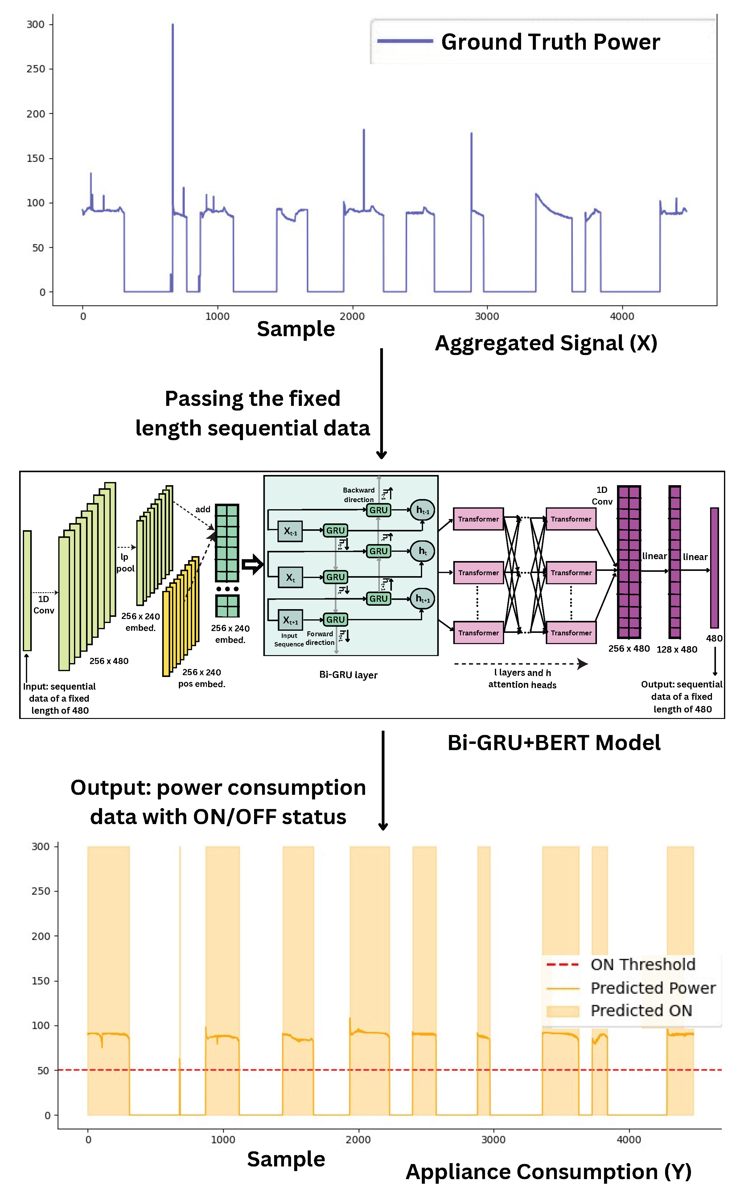
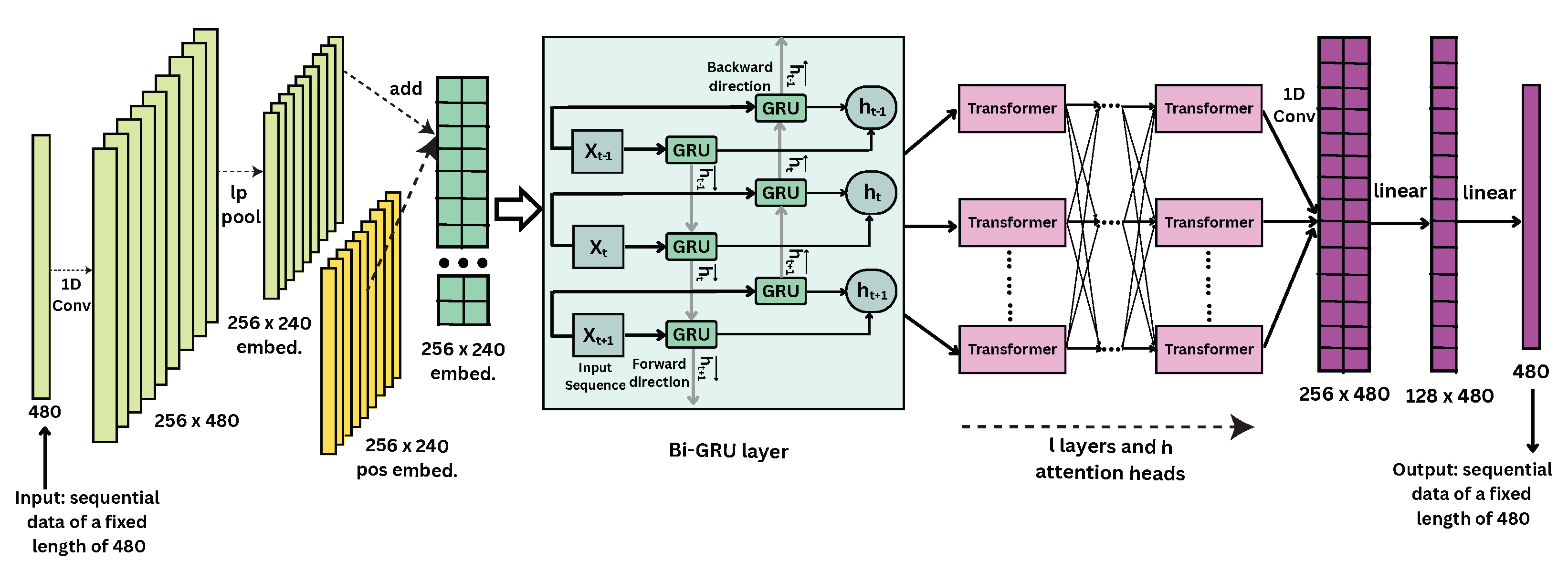
In this work, we propose a novel improved hybrid deep learning NILM approach based on GRU and BERT, which performs per-appliance prediction of both the power consumption and ON/OFF status of individual appliances. We develop two models that separately combine BERT with unidirectional and bidirectional variants of GRU (Our proposed models’ implementations are available at https://github.com/AnnyshaHuzzat/GRU-BERT-for-NILM, accessed on 16 September 2025). We later demonstrate in the results section that the Bi-GRU+BERT model consistently outperforms the GRU+BERT variant after 20 epochs of training, matching the training conditions used by most state-of-the-art baselines. Therefore, in this section, we focus on detailing the architecture of the Bi-GRU+BERT model. As illustrated in Figure 1, our model processes a fixed-length input sequence of 480 aggregate power readings and outputs the disaggregated power consumption with the same temporal resolution. Our proposed architecture, illustrated in Figure 2, consists of four main components: a feature extraction and positional embedding module, a Bi-GRU layer, transformer blocks, and a multi-layer decoder.

3.1. Feature Extraction and Embedding Module

The Feature Extraction and Embedding Module serves as the initial processing stage for the one-dimensional (1D) aggregate power input in NILM tasks. Its primary objective is to extract meaningful temporal patterns from the input signal, enabling the model to learn distinct appliance behaviors based on local power variations and signal dynamics.

We begin with an input sequence $X\in {\mathbb{R}}^{T\times 1}$ (e.g., 480 aggregate power readings), where $\mathbb{R}$ denotes the set of real numbers, T is the sequence length, and each value represents a real-valued power measurement at a time step. The feature extraction process begins with a 1D convolutional layer that applies 256 filters to detect localized temporal features, such as sharp power spikes, short bursts, and ON/OFF transitions. This operation increases the representational dimensionality and enables the model to learn a diverse set of discriminative features.

Next, the convolutional output is passed through L2-pooling, a specific case of $L_p$-pooling with $p=2$ using a kernel size of 2 and stride of 2, which halves the sequence length while preserving the most informative signal characteristics. This operation is defined in (1):

$$\mathrm{L}2\mathrm{Pool}{\left(\mathrm{Conv}1\mathrm{D}\left(X\right)\right)}_j=\sqrt{\sum _{i\in {\mathrm{window}}_j}{\left|\mathrm{Conv}1\mathrm{D}{\left(X\right)}_i\right|}^2},$$

(1)

where $\mathrm{Conv}1\mathrm{D}{\left(X\right)}_i$ are the output values of the 1D convolution layer within each pooling window, and ${\mathrm{window}}_j$ indicates the pooling window corresponding to the output index j. No additional normalization is applied within each pooling window, as the relative magnitude of features is crucial for NILM tasks and the normalization could suppress the sharp power spikes or ON/OFF transitions that are key indicators of appliance activity. Retaining the true magnitudes allows the subsequent Bi-GRU and transformer layers to more accurately learn appliance-specific temporal patterns. By using this pooling method, the model preserves the most relevant features while discarding redundant or noisy information. This reduction in sequence length allows the model to concentrate on relevant patterns in the signal, facilitating a more focused and effective temporal learning in subsequent layers.

To encode the input signal while preserving temporal ordering, which is essential for time-series tasks but not natively captured by transformer-based models, a learnable positional embedding matrix $E_{\mathrm{pos}}\in {\mathbb{R}}^{T^{\prime }\times d_{\mathrm{emb}}}$ is added to the pooled features, where $d_{\mathrm{emb}}=256$ is the feature dimension after the Conv1D and L2-pooling operations. This embedding injects relative positional information, allowing the model to differentiate between events that occur at different times in the sequence. The result is then passed through layer normalization to stabilize the feature distribution and ensure consistent gradients during training. A dropout layer with a probability of 0.1 is applied afterward to prevent overfitting and encourage robust feature learning.

The final embedded representation $X^{\prime }\in {\mathbb{R}}^{T^{\prime }\times d_{\mathrm{emb}}}$ shown in (2) serves as input to the subsequent Bi-GRU layer for sequential temporal modeling purpose.

$$\begin{array}{ccc}& & X^{\prime }=\mathrm{Dropout}\left(\mathrm{LayerNorm}\left(\mathrm{L}2\mathrm{Pool}\left(\mathrm{Conv}1\mathrm{D}\left(X\right)\right)+E_{\mathrm{pos}}\right)\right)\hfill \\ & & \mathrm{with}X\in {\mathbb{R}}^{T\times 1},E_{\mathrm{pos}}\in {\mathbb{R}}^{T^{\prime }\times d_{\mathrm{emb}}}\hfill \end{array}$$

(2)

3.2. Bidirectional GRU Layer

The output of the embedding module is passed to a Bi-GRU layer with 256 hidden units in each direction, resulting in a combined hidden size of 512. This configuration balances between model complexity and expressiveness, providing enough capacity to capture both forward and backward temporal dependencies. By processing the input in both directions, the GRU effectively identifies complex patterns in energy consumption data, such as transient spikes and recurring usage patterns, which are crucial for accurate disaggregation in NILM tasks [27].

Integrating the Bi-GRU layer before the transformer encoder enables the model to first capture the local sequential dependencies, which form the foundation for more complex attention-based contextual learning in the transformer [9]. This two-stage approach, which is commonly used in sequence modeling, allows the GRU to handle short-term patterns, while the transformer focuses on long-range dependencies and feature interactions.

Given the input sequence $X^{\prime }=(x_1,x_2,\dots ,x_T)$ from the previous module, the GRU computes a sequence of hidden states as follows:

$$H=\mathrm{BiGRU}\left(X^{\prime }\right)=\left[\overrightarrow{h_t}\parallel \overleftarrow{h_t}\right],t=1,\dots ,T$$

(3)

where $\overrightarrow{h_t}$ and $\overleftarrow{h_t}$ represent the forward and backward hidden states at time t, respectively, T denotes the sequence length, and ‖ denotes concatenation. The GRU output H is then passed to the transformer encoder for further temporal modeling.

3.3. Transformer Blocks

The input to the transformer blocks is the output $H\in {\mathbb{R}}^{T\times d_h}$ from the Bi-GRU layer, where $d_h$ is the hidden size of each time step (in our case, $d_h=512$). Each hidden state $h_t\in {\mathbb{R}}^{d_h}$ captures rich bidirectional temporal features that serve as input for the attention mechanism.

In order to enable the model to selectively focus on different parts of the input sequence, H is linearly projected into three separate matrices, namely, queries Q, keys K, and values V, defined in (4) as

$$Q=H{W}^Q,K=H{W}^K,V=H{W}^V$$

(4)

Here, $W^Q,W^K,W^V\in {\mathbb{R}}^{d_h\times d_k}$ are trainable weight matrices, and $d_k$ is the dimensionality of the query and key vectors for each attention head. Typically, $d_k=d_h/n$, where n is the number of attention heads.

3.3.1. Attention Mechanism

The core operation of the attention mechanism is the scaled dot-product attention, which computes similarity scores between query and key vectors and uses them to weight the values. This is formally defined in (5) as follows:

$$\mathrm{Attention}(Q,K,V)=\mathrm{softmax}\left({\displaystyle \frac{Q{K}^T}{\sqrt{d_k}}}\right)V$$

(5)

3.3.2. Multi-Head Attention Layer

To capture information from multiple subspaces, the model uses multi-head attention, where this attention mechanism is repeated n times in parallel with independent projections. The resulting outputs from each head are concatenated and passed through a final linear transformation, shown in (6) below:

$$\mathrm{MultiHead}(Q,K,V)=\left({\parallel }_{i=1}^n{\mathrm{head}}_i\right)W^O$$

(6)

In this equation, ${\mathrm{head}}_i=\mathrm{Attention}(Q_i,K_i,V_i)$ is the output of the i-th attention head, ‖ denotes concatenation along the feature dimension, and $W^O\in {\mathbb{R}}^{n·d_k\times d_h}$ is a learned output projection matrix that maps the concatenated output back to the model’s hidden size.

By computing attention across multiple heads, the model can learn diverse contextual relationships within the input sequence, enhancing its ability to identify patterns in power consumption data across various temporal scales. The output of this module is denoted as $M{H}_{\mathrm{attn}}=\mathrm{MultiHead}(Q,K,V)\in {\mathbb{R}}^{T\times d_h}$, which serves as the input to the subsequent feed-forward network.

3.3.3. Feed-Forward Network

The output from the multi-head attention layer $M{H}_{\mathrm{attn}}$ is then passed through a position-wise feed-forward network (PFFN), which consists of two linear transformations separated by a non-linear activation function. This operation is defined in (7) as follows:

$$\mathrm{PFFN}\left(M{H}_{\mathrm{attn}}\right)=\mathrm{GELU}(M{H}_{\mathrm{attn}}{W}_1+b_1)W_2+b_2$$

(7)

Here, $W_1\in {\mathbb{R}}^{d_h\times d_{ff}}$ and $W_2\in {\mathbb{R}}^{d_{ff}\times d_h}$ are learnable weight matrices, while $b_1$ and $b_2$ are their corresponding bias vectors. The parameter $d_{ff}$ represents the intermediate dimensionality of the feed-forward network and is typically larger than the model’s hidden size $d_h$, e.g., $d_{ff}=2048$. This projection into a higher-dimensional space allows the network to capture more expressive feature interactions before reducing the output back to the original hidden size.

The activation function used is the Gaussian Error Linear Unit (GELU), which introduces non-linearity and enables the network to learn complex and expressive transformations. Each transformer block also incorporates residual connections, layer normalization, and dropout, which together improve the training stability and reduce the risk of overfitting.

3.4. Decoder and Output Layers

The final output of the transformer block, after applying the PFFN to the multi-head attention output, is denoted as $H_{\mathrm{trans}}=\mathrm{PFFN}\left(M{H}_{\mathrm{attn}}\right)\in {\mathbb{R}}^{T\times d_h}$, where $d_h=512$ (after the transformer block). This output encodes the rich contextual and sequential representations of the appliance-level power consumption.

3.4.1. Power Consumption Prediction

To restore the temporal resolution of the sequence, the sequence that was previously downsampled by L2 pooling during feature extraction $H_{\mathrm{trans}}$ is passed through a transposed convolutional layer, denoted as $\mathrm{Deconv}\left(H_{\mathrm{trans}}\right)$. The transposed convolution uses a kernel size of 4, stride of 2, and padding of 1, which exactly inverts the downsampling performed by the L2 pooling layer. This layer upsamples the sequence back to its original length $T_{\mathrm{orig}}$, aligning it with the input resolution for frame-wise predictions.

The upsampled sequence is then processed by two fully connected (linear) layers. The first layer, ${\mathrm{Linear}}_1$, reduces the feature dimensionality from 256 to 128 and applies a non-linear activation function $\tan \mathrm{h}$, which introduces bounded non-linearity and helps to model subtle variations in power levels. The second layer, ${\mathrm{Linear}}_2$, maps the intermediate representation to a single scalar value per time step, yielding the predicted power consumption as expressed in (8).

$$\widehat{Y}={\mathrm{Linear}}_2\left(tanh\left({\mathrm{Linear}}_1\left(\mathrm{Deconv}\left(H_{\mathrm{trans}}\right)\right)\right)\right)$$

(8)

Here, we denote $H_{\mathrm{trans}}=\mathrm{PFFN}\left(M{H}_{\mathrm{attn}}\right)\in {\mathbb{R}}^{T\times d_h}$, and $\mathrm{Deconv}\left(H_{\mathrm{trans}}\right)\in {\mathbb{R}}^{T_{\mathrm{orig}}\times d_h}$, where the transposed convolution restores the input sequence length ($T_{\mathrm{orig}}=480$). The first fully connected layer is defined as ${\mathrm{Linear}}_1:{\mathbb{R}}^{d_h}\to {\mathbb{R}}^{128}$. This is followed by a tanh activation. This is then passed to the second linear layer, ${\mathrm{Linear}}_2:{\mathbb{R}}^{128}\to {\mathbb{R}}^1$. This outputs the predicted normalized power value at each time step.

The resulting output sequence is $\widehat{Y}=[{\widehat{Y}}_1,{\widehat{Y}}_2,\dots ,{\widehat{Y}}_{T_{\mathrm{orig}}}]\in {\mathbb{R}}^{T_{\mathrm{orig}}\times 1}$, where ${\widehat{Y}}_t$ denotes the predicted normalized power at a time step t. These values are then rescaled by multiplying with the maximum rated power of the target appliance, $P_{\max }$ (defined as “Max. Limit” in

Table 2. Preprocessing of the UK-DALE (upper) and REDD (lower) datasets. For UK-DALE, ON/OFF thresholds, maximum power limits, and minimum durations for each appliance are adopted from the prior literature [7,8,9] to maintain a fair comparison with existing NILM studies. For REDD, the thresholds and parameters are chosen based on our experimental settings.

Appliance	$\mathit{\lambda }$	Max. Limit (W)	ON Ths. (W)	Min. ON Duration (s)	Min. OFF Duration (s)
Fridge	${10}^{-6}$	300	50	60	12
Washer	${10}^{-2}$	2500	20	1800	160
Microwave	1	3000	200	12	30
Dishwasher	1	2500	10	1800	1800
Kettle	1	3100	2000	12	0
Fridge	${10}^{-6}$	400	50	60	12
Microwave	1	1800	200	12	30
Dishwasher	1	1200	10	300	300

), to obtain the final power consumption prediction:

$${\widehat{y}}_t=min\left({\widehat{Y}}_t·P_{\max },P_{\max }\right)$$

(9)

The clamping operation, denoted by the $min(·)$ function in (9), ensures that the predicted power at any time step t does not exceed the appliance’s rated capacity, maintaining physical plausibility. This means that the predicted power values respect the maximum rated capacity of the appliance. For instance, a kettle rated at 2000 W cannot physically consume more than 2000 W, so predictions are bounded accordingly. The operation prevents the model from producing nonphysical spikes in power consumption. Importantly, this clamping does not meaningfully bias the MAE downward. The MAE is only affected if predictions exceed the appliance’s rated power, which is rare under proper model training with normalized data. Most predictions remain below the rated power, so the clamping has minimal impact on the error.

3.4.2. ON/OFF  Classification. It is fine.

To infer the binary ON/OFF status, a thresholding operation is applied to the predicted power signal. Specifically, for each time step t, the appliance is considered ON if ${\widehat{y}}_t\ge \theta$, where $\theta$ is an appliance-specific threshold value determined by empirical analysis from [7]. This process is summarized as follows:

$${\mathrm{ON}}_t=\left\{\begin{array}{cc}1,\hfill & \mathrm{if}{\widehat{y}}_t\ge \theta \hfill \\ 0,\hfill & \mathrm{otherwise}\hfill \end{array}\right.$$

(10)

Here, the threshold values for each appliance are denoted in Table 2 as (“ON Ths.”). This postprocessing step enables the model to jointly provide both continuous power estimates and binary ON/OFF classification, aligning with real-world NILM deployment needs.

4. Experimental Setup, Results, and Benchmarking

4.1. Objective Function

Following prior baselines [7,8,9], we adopt a composite objective function for both models, which combines Kullback–Leibler (KL) divergence, mean squared error (MSE), soft margin loss for ON/OFF state prediction, and a weighted L1 loss to better capture rare activation events. The total loss is given by

$${\mathcal{L}}_{\mathrm{total}}={\mathcal{L}}_{\mathrm{KL}}+{\mathcal{L}}_{\mathrm{MSE}}+{\mathcal{L}}_{\mathrm{margin}}+C_0·{\mathcal{L}}_{\mathrm{L}1-\mathrm{on}},$$

(11)

where the first three terms are equally weighted with a fixed coefficient of $1.0$, and $C_0$ is an appliance-specific hyperparameter (denoted as $\lambda$ in Table 2) that controls the contribution of the ON-state penalty.

The KL divergence term is defined as

$${\mathcal{L}}_{\mathrm{KL}}=D_{\mathrm{KL}}\left(log\mathrm{Softmax}\left(\frac{\widehat{y}}{\tau }\right)\parallel \mathrm{Softmax}\left(\frac{y}{\tau }\right)\right),$$

(12)

where $\widehat{y}$ and y are the predicted and true normalized energy values, and $\tau =0.1$ is a temperature parameter that smooths the softmax distributions to mitigate the imbalance between ON and OFF events.

The MSE loss is expressed as

$${\mathcal{L}}_{\mathrm{MSE}}={\displaystyle \frac{1}{N}}\sum _{i=1}^N{\left({\widehat{y}}_i-y_i\right)}^2,$$

(13)

which penalizes deviations between predicted and ground-truth power values over a sequence of length N.

To ensure reliable detection of appliance states, the soft margin loss is used:

$${\mathcal{L}}_{\mathrm{margin}}={\displaystyle \frac{1}{N}}\sum _{i=1}^{N}log\left(1+exp\left(-s_i·{\widehat{s}}_i\right)\right),$$

(14)

where $s_i\in \{-1,1\}$ are the ground truth ON/OFF labels and ${\widehat{s}}_i\in \{-1,1\}$ are the predicted states. This formulation penalizes incorrect state classification while being robust to class imbalance.

Finally, the ON-state weighted L1 loss is defined as

$${\mathcal{L}}_{\mathrm{L}1-\mathrm{on}}={\displaystyle \frac{1}{\left|M\right|}}\sum _{i\in M}\left|{\widehat{y}}_i-y_i\right|,$$

(15)

where M denotes the set of time steps where the appliance is active ($s_i=1$) or misclassified. This term enforces additional penalty on prediction errors during critical ON periods. Its influence is scaled by $C_0$, which is tuned per appliance based on its activation frequency and normalized by $\left|M\right|$ to prevent overweighting.

This explicit formulation ensures that the model jointly optimizes for accurate energy estimation (${\mathcal{L}}_{\mathrm{MSE}}$), distributional similarity (${\mathcal{L}}_{\mathrm{KL}}$), and reliable ON/OFF detection (${\mathcal{L}}_{\mathrm{margin}}$) while emphasizing infrequent but important ON-state events ($C_0·{\mathcal{L}}_{\mathrm{L}1-\mathrm{on}}$). Table 2 reports the specific $C_0$ values used in our experiments. The model is optimized using Adam with fixed hyperparameters, and we investigate the effect of varying epoch lengths on disaggregation performance, particularly for low-frequency appliance events.

4.2. Dataset Preprocessing

The UK Domestic Appliance-Level ELECTRIcity (UK-DALE) [22] dataset provides detailed energy usage data from five UK households, including both aggregate mains and individual appliance readings. We use low-frequency data for five appliances, namely, refrigerator, washer–dryer, microwave, dishwasher, and kettle. All signals are resampled to six-second intervals with forward-filling applied for gaps under three minutes, ensuring temporal alignment between mains and appliance-level data.

The Reference Energy Disaggregation Dataset (REDD) [23] is a benchmark NILM dataset widely used for evaluating appliance-level energy disaggregation. For the REDD dataset, we use the preprocessed data from [28], where thresholds and parameters are chosen based on experimental settings.

As shown in Table 2, raw readings are clamped using appliance-specific power limits to remove unrealistic spikes. Ground-truth labels are generated by applying ON-thresholds and enforcing minimum ON/OFF durations, stabilizing detection of true activations. For instance, the kettle uses a high ON-threshold (2000 W) with no OFF-delay, while the dishwasher requires sustained activity to be considered “on”.

The regularization parameter ($\lambda$) helps prevent overfitting by penalizing large model weights. It is assigned based on appliance activity levels: higher values, e.g., 1, are used for frequently active appliances like the microwave to constrain overfitting, while lower values, e.g., ${10}^{-6}$, allow more flexibility for sparsely active ones like the fridge. Aggregated main signals are normalized using training-set statistics to ensure consistency during evaluation.

4.3. Training Details

The proposed Bi-GRU+BERT and GRU+BERT models are trained in a supervised manner using disaggregated ground-truth appliance-level power data using a masked learning strategy inspired by the Masked Language Model (MLM) of BERT [20]. For each input sequence of length 480, a masking ratio $p=0.25$ is applied by randomly replacing elements with a special token. The model is trained to predict only these masked positions, encouraging it to learn contextual dependencies across the sequence [7].

To enhance temporal modeling, both variants incorporate a GRU-based layer before the transformer encoder. The GRU+BERT model uses a unidirectional GRU with 256 hidden units, resulting in a 256-dimensional contextual embedding. In contrast, the Bi-GRU+BERT model employs a bidirectional GRU with 256 hidden units in each direction, producing a 512-dimensional contextual embedding by concatenating forward and backward outputs. Both models are optimized using the Adam optimizer with a learning rate of ${10}^{-4}$, $\beta$ values of (0.9, 0.999), and no weight decay, enabling efficient and stable convergence for deep sequential learning [7,8,9,25].

Input sequences are normalized using the mean and standard deviation from the training set, and the same parameters are applied during evaluation to ensure consistent input scaling. For evaluation, we adopt a house-based split of the UK-DALE dataset: houses 1, 3, 4, and 5 are used for training, 20% of house 1 for validation, and house 2 (unseen) for testing. Appliance labels are generated using predefined thresholds, ensuring generalization and preventing data leakage. Similarly, for the REDD dataset, houses 2, 3, 4, 5, and 6 are used for training, house 2 for validation, and house 1 (unseen) for testing. As the REDD dataset is smaller than the UK-DALE, prior benchmark models were typically trained for up to 100 epochs. In our case, we employed an early stopping strategy: if the validation loss did not decrease for more than five consecutive epochs, training was halted to prevent overfitting.

4.4. Evaluation and Benchmarking

In this subsection, we evaluate the performance of our proposed models for the NILM task using real household smart meter data. Our evaluation is conducted on the UK-DALE and REDD datasets using four standard evaluation metrics: accuracy, F1-score, mean relative error (MRE), and mean absolute error (MAE). These metrics are chosen because they are widely used in previous benchmark studies, allowing for a direct and meaningful comparison with existing methods.

Accuracy measures the proportion of correctly predicted ON/OFF states of an appliance among all predictions:

$$\mathrm{Accuracy}={\displaystyle \frac{TP+TN}{TP+TN+FP+FN}}$$

where $TP$, $TN$, $FP$, and $FN$ denote the number of true positives, true negatives, false positives, and false negatives, respectively.

F1-score is the harmonic mean of precision and recall, providing a balanced measure of model performance for imbalanced datasets:

$$\mathrm{F}1\mathrm{-score}=2·{\displaystyle \frac{\mathrm{Precision}·\mathrm{Recall}}{\mathrm{Precision}+\mathrm{Recall}}},\mathrm{Precision}={\displaystyle \frac{TP}{TP+FP}},\mathrm{Recall}={\displaystyle \frac{TP}{TP+FN}}$$

Mean absolute error (MAE) quantifies the average magnitude of the error between predicted and true power values (in watts) without considering the direction of the error:

$$\mathrm{MAE}={\displaystyle \frac{1}{N}}\sum _{i=1}^N|y_i-{\widehat{y}}_i|$$

where $y_i$ and ${\widehat{y}}_i$ are the true and predicted power consumption at time step i, and N is the total number of predictions.

Mean relative error (MRE) measures the average relative difference between the predicted and true power values, providing a normalized error metric:

$$\mathrm{MRE}={\displaystyle \frac{1}{N}}\sum _{i=1}^N{\displaystyle \frac{|y_i-{\widehat{y}}_i|}{y_i}}$$

This metric is especially useful for comparing errors across appliances with different power ranges.

In the following, we benchmark the performance of our models against several state-of-the-art baselines, including GRU+ [9], LSTM+ [9], CNN [9], BERT4NILM [7], ELECTRIcity [8], and CTA-BERT [9].

4.4.1. Training Results

To establish a fair comparison, we first trained the publicly available models BERT4NILM [7] and ELECTRIcity [8] and then compared their performance with that of our proposed models. BERT4NILM was trained for 20 epochs following its original implementation [7], which aligns with the configuration used for our proposed GRU+BERT and Bi-GRU+BERT models. On the other hand, ELECTRIcity [8] was trained for 90 epochs as specified in its original implementation in [8].

Table 3. Training performance of BERT4NILM, ELECTRIcity, the proposed Bi-GRU+BERT, and its variant GRU+BERT across five appliances from the UK-DALE dataset. Models are evaluated using accuracy, F1-score, MAE, and MRE, where MAE is reported in normalized units, i.e., values between 0 and 1. The number of training epochs and total training time (in minutes) are also reported. The best results are highlighted in bold.

Appliance	Model	Epochs	Accuracy	F1-Score	MAE	MRE	Train Time (Min)
Kettle	BERT4NILM	20	0.996	0.884	0.002	3.801	108.20
	ELECTRIcity	90	0.999	0.945	0.002	3.762	106.34
	GRU+BERT (proposed)	20	0.998	0.883	0.008	15.342	105.12
	Bi-GRU+BERT (proposed)	20	0.994	0.897	0.007	15.156	108.23
Fridge	BERT4NILM	20	0.823	0.765	0.217	19.594	116.55
	ELECTRIcity	90	0.867	0.834	0.618	19.332	118.45
	GRU+BERT (Proposed)	20	0.913	0.904	0.099	8.768	118.23
	Bi-GRU+BERT (proposed)	20	0.928	0.914	0.098	8.424	118.34
Washing machine	BERT4NILM	20	0.996	0.644	0.067	6.98	115.55
	ELECTRIcity	90	0.996	0.843	0.010	3.81	119.13
	GRU+BERT (proposed)	20	0.997	0.894	0.037	6.567	115.44
	Bi-GRU+BERT (proposed)	20	0.994	0.938	0.024	6.266	117.43
Microwave	BERT4NILM	20	0.996	0.697	0.005	4.455	112.34
	ELECTRIcity	90	0.996	0.677	0.006	4.532	119.32
	GRU+BERT (proposed)	20	0.996	0.543	0.007	4.155	118.33
	Bi-GRU+BERT (proposed)	20	0.997	0.736	0.005	3.982	119.12
Dishwasher	BERT4NILM	20	0.967	0.745	0.053	6.521	118.23
	ELECTRIcity	90	0.988	0.819	0.011	7.878	118.43
	GRU+BERT (proposed)	20	0.976	0.810	0.014	3.431	115.43
	Bi-GRU+BERT (proposed)	20	0.985	0.748	0.015	4.989	116.42

presents the detailed training results for five common appliances: kettle, fridge, washing machine, microwave, and dishwasher. The results demonstrate that our proposed models consistently achieve a competitive performance in terms of all four metrics while maintaining comparable training times.

All models were trained using an NVIDIA A100 GPU, and the corresponding training times are reported to ensure transparency and reproducibility. The best results for each model were obtained after several training runs to ensure stability. This training analysis, which is reported in Table 3, serves two purposes: (1) to identify signs of overfitting by examining discrepancies between training and test scores; and (2) to evaluate the training efficiency in terms of convergence speed and computational overhead. These insights help highlight the trade-offs between performance and practicality, particularly in real-world NILM deployments where fast, efficient training is critical.

In

Table 4. Model complexity and approximate inference cost per input window (UK-DALE window = 480 samples). GPU times are for NVIDIA A100.

Model	Total Params	Trainable	FLOPs/Window	Memory (MB)	CPU (ms)	A100 (ms)
BERT4NILM	1,895,425	1,895,425	35.40 GFLOPs	11.18	12	0.3
GRU+BERT	2,290,177	2,290,177	60.66 GFLOPs	12.89	18	0.5
Bi-GRU+BERT	7,674,369	7,674,369	124.20 GFLOPs	37.43	42	1.0
ELECTRICITY	2,081,730	2,081,730	136.49 GFLOPs	51.18	45	1.0

, we summarize the model complexity and computational cost of the compared approaches, reporting trainable parameters, approximate floating-point operations per second (FLOPs) per input window, memory usage, and wall-clock inference times on the CPU and NVIDIA A100 GPU. Our analysis shows that Bi-GRU+BERT has the highest parameter count, which is approximately four times and three times that of BERT4NILM and GRU+BERT, respectively, while ELECTRICITY exhibits high FLOPs despite the lowest number of parameters, indicating more expensive per-sample operations. Memory usage follows a similar trend, with Bi-GRU+BERT requiring less memory than ELECTRICITY but more than the other baselines. Inference times on both the CPU and GPU scale are approximately consistent with FLOPs, where both proposed models are consistently faster than ELECTRICITY on the GPU, and GRU+BERT is also faster on the CPU.

In addition, training times per epoch on A100 remain comparable across models, suggesting that the increased model size does not lead to prohibitive training overhead. These results indicate that the model complexity, while higher for Bi-GRU+BERT, does not translate into impractical deployment constraints compared to the existing models. Specifically, GRU+BERT achieves strong predictive performance with modest computational cost, requiring only 18 ms per input window on the CPU and 0.5 ms on the GPU, making it well-suited for resource-limited environments such as residential smart meters. Bi-GRU+BERT, while larger and more computationally intensive, achieves the highest predictive accuracy and still maintains real-time GPU inference (1 ms per window) and reasonable CPU inference (42 ms per window). Therefore, both models are viable for practical NILM deployment: GRU+BERT provides an efficient and lighter-weight solution for residential scenarios, whereas Bi-GRU+BERT is more suitable when higher accuracy is prioritized and GPU acceleration is available.

4.4.2. Test Results

We benchmark the test performance of our models against several state-of-the-art baselines. As shown in

Table 5. Test results on the UK-DALE dataset for the kettle. Here, MAE is reported in watts (W). The best results are highlighted in bold.

Model	Number of Epochs	Accuracy	F1-Score	MRE	MAE (W)
GRU+ (reported from [9])	20	0.993	0.425	0.008	23.22
LSTM+ (reported from [9])	20	0.994	0.531	0.007	21.26
CNN (reported from [9])	20	0.997	0.850	0.003	9.64
BERT4NILM (reported from [7])	20	0.998	0.907	0.002	6.82
BERT4NILM (from our training)	20	0.995	0.667	0.006	18.32
CTA-BERT (reported from [9])	20	0.999	0.963	0.001	3.36
GRU+BERT (proposed)	20	0.997	0.798	0.005	12.09
Bi-GRU+BERT (proposed)	20	0.997	0.804	0.005	11.92
ELECTRIcity (reported from [8])	90	0.999	0.939	0.003	9.26
ELECTRIcity (from our training)	90	0.999	0.921	0.004	10.54
GRU+BERT (proposed)	60	0.997	0.799	0.005	12.18
Bi-GRU+BERT (proposed)	60	0.997	0.798	0.005	12.18

,

Table 6. Test results on the UK-DALE dataset for the fridge. Here, MAE is reported in watts (W). The best results are highlighted in bold.

Model	Number of Epochs	Accuracy	F1-Score	MRE	MAE (W)
GRU+ (reported from [9])	20	0.636	0.401	0.901	39.54
LSTM+ (reported from [9])	20	0.573	0.174	0.956	43.74
CNN (reported from [9])	20	0.772	0.718	0.758	29.20
BERT4NILM (reported from [7])	20	0.813	0.766	0.732	25.49
BERT4NILM (from our training)	20	0.841	0.810	0.699	22.30
CTA-BERT (reported from [9])	20	0.812	0.796	0.608	25.32
GRU+BERT (proposed)	20	0.887	0.871	0.646	17.68
Bi-GRU+BERT (proposed)	20	0.889	0.871	0.649	17.69
ELECTRIcity (reported from [8])	90	0.843	0.810	0.706	22.61
ELECTRIcity (from our training)	90	0.837	0.805	0.703	22.40
GRU+BERT (proposed)	60	0.888	0.870	0.652	17.48
Bi-GRU+BERT (proposed)	60	0.877	0.856	0.653	18.052

,

Table 7. Test results on the UK-DALE dataset for the washing machine. Here, MAE is reported in watts (W). The best results are highlighted in bold.

Model	Number of Epochs	Accuracy	F1-Score	MRE	MAE (W)
GRU+ (reported from [9])	20	0.342	0.018	0.662	68.65
LSTM+ (reported from [9])	20	0.938	0.150	0.067	15.66
CNN (reported from [9])	20	0.913	0.173	0.094	11.90
BERT4NILM (reported from [7])	20	0.966	0.325	0.040	6.98
BERT4NILM (from our training)	20	0.991	0.616	0.014	4.33
CTA-BERT (reported from [9])	20	0.959	0.340	0.046	8.83
GRU+BERT (proposed)	20	0.992	0.765	0.015	6.86
Bi-GRU+BERT (proposed)	20	0.993	0.765	0.015	6.86
ELECTRIcity (reported from [8])	90	0.994	0.797	0.011	3.65
ELECTRIcity (from our training)	90	0.996	0.835	0.011	3.84
GRU+BERT (proposed)	60	0.996	0.877	0.010	5.44
Bi-GRU+BERT (proposed)	60	0.996	0.857	0.011	4.96

,

Table 8. Test results on the UK-DALE dataset for the microwave. Here, MAE is reported in watts (W). The best results are highlighted in bold.

Model	Number of Epochs	Accuracy	F1-Score	MRE	MAE (W)
GRU+ (reported from [9])	20	0.996	0.266	0.014	6.41
LSTM+ (reported from [9])	20	0.995	0.060	0.014	6.55
CNN (reported from [9])	20	0.995	0.341	0.014	6.57
BERT4NILM (reported from [7])	20	0.995	0.014	0.014	6.57
BERT4NILM (from our training)	20	0.995	0.002	0.014	6.57
CTA-BERT (reported from [9])	20	0.996	0.209	0.013	6.27
GRU+BERT (proposed)	20	0.995	0.229	0.014	6.25
Bi-GRU+BERT (proposed)	20	0.996	0.515	0.013	5.59
ELECTRIcity (reported from [8])	90	0.996	0.277	0.013	6.28
ELECTRIcity (from our training)	90	0.995	0.152	0.014	6.47
GRU+BERT (proposed)	60	0.996	0.553	0.013	5.24
Bi-GRU+BERT (proposed)	60	0.995	0.361	0.014	6.02

and

Table 9. Test results on the UK-DALE dataset for the dishwasher. Here, MAE is reported in watts (W). The best results are highlighted in bold.

Model	Number of Epochs	Accuracy	F1-Score	MRE	MAE (W)
GRU+ (reported from [9])	20	0.977	0.639	0.035	38.42
LSTM+ (reported from [9])	20	0.976	0.560	0.029	35.25
CNN (reported from [9])	20	0.947	0.560	0.026	25.94
BERT4NILM (reported from [7])	20	0.966	0.667	0.049	16.18
BERT4NILM (from our training)	20	0.996	0.665	0.051	17.15
CTA-BERT (reported from [9])	20	0.979	0.669	0.042	13.32
GRU+BERT (proposed)	20	0.981	0.777	0.030	17.68
Bi-GRU+BERT (proposed)	20	0.980	0.687	0.028	27.42
ELECTRIcity (reported from [8])	90	0.984	0.818	0.028	18.96
ELECTRIcity (from our training)	90	0.985	0.789	0.024	18.99
GRU+BERT (proposed)	60	0.978	0.750	0.033	24.71
Bi-GRU+BERT (proposed)	60	0.980	0.688	0.025	23.69

, we provide an appliance-wise comparison across the four evaluation metrics, enabling a comprehensive assessment of both accuracy and generalization. These test results are critical in confirming that our proposed models not only perform well on the training data but also can generalize effectively to unseen scenarios, which is an essential requirement for real-world NILM applications. Moreover we determined the optimal hyperparameters through a combination of manual tuning and by aligning with configurations commonly used in recent transformer-based NILM studies [7,8,9,25], ensuring both fair comparison and optimal performance in our specific setup. We also acknowledge that reproduced results for these baselines may vary slightly from the originally reported numbers due to differences in initialization, data preprocessing, train/test splits, and implementation details, which are often not fully specified in the original publications.

To maintain consistency with previous state-of-the-art models, we initially trained our models for 20 epochs, following common practices reported in prior works such as GRU+, LSTM+, CNN, CTA-BERT, and BERT4NILM. The reported results for GRU+, LSTM+, CNN, and CTA-BERT were taken from [9]. For BERT4NILM [7] and ELECTRIcity [8], we utilized the publicly available code to reproduce and evaluate them on our setup and also provide the results reported in their original implementations. Table 5, Table 6, Table 7, Table 8 and Table 9 present the performance of all models on the UK-DALE test set, with the best results highlighted in bold.

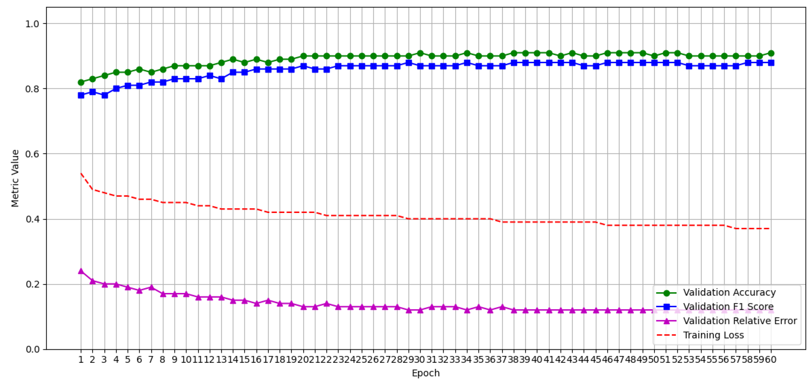
Additionally, to conduct a more comprehensive comparison with models trained for longer durations such as ELECTRIcity [8], which was trained for 90 epochs, we extended our training until the error rates of our proposed models reached convergence, which occurred around 60 epochs, as shown in Figure 3. With this extended training, our models outperformed ELECTRIcity [8] across all appliances except for the kettle and dishwasher, where they achieved comparable performance. Moreover, our training budget reflects realistic NILM deployment settings, where faster convergence and lower computational overhead are key performance indicators [29,30]. Even within these constraints, our models consistently demonstrate robust generalization and competitive performance.

As shown in Table 5 for the kettle, GRU+BERT and Bi-GRU+BERT attain F1-scores of 0.798 and 0.804, respectively, with accuracy at 0.997 and low MRE and MAE values. Although slightly behind CTA-BERT in F1-score, our models still deliver highly reliable disaggregation with minimal error—especially considering the short duration and high-frequency switching nature of kettle usage. These brief and abrupt power bursts are harder to detect consistently, which may explain the slight drop in F1-score compared to models [9] specifically designed with mechanisms such as time-aware masking or dilation for capturing transient behaviors.

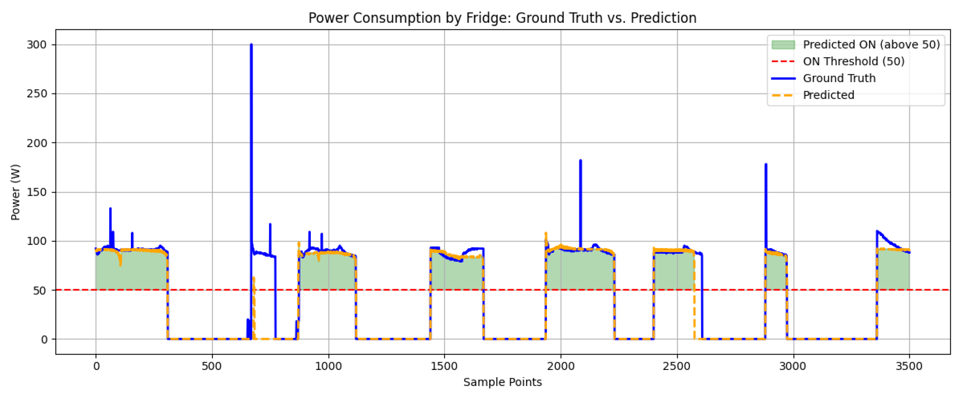
The fridge results in Table 6 show that both GRU+BERT and Bi-GRU+BERT outperform existing approaches, achieving the highest F1-scores (0.871) and improved accuracy (0.887 and 0.889). Despite being trained for significantly fewer epochs, our proposed models surpass other models, demonstrating their robustness in detecting long, continuous appliance cycles. Figure 4 further illustrates the effectiveness of the Bi-GRU+BERT model in tracking real-time fridge power usage and corresponding ON/OFF states, capturing the cyclical nature of the appliance with high temporal accuracy.

The performance of the washing machine is summarized in Table 7, where both of our proposed models, trained for 20 epochs, demonstrate substantial improvements over the baseline methods. They achieve F1-scores of 0.765 and maintain high accuracy levels of 0.992 and 0.993, respectively. Additionally, both models achieve comparatively low MRE values (0.015), indicating strong precision in estimating appliance-level power consumption. These results suggest that the combination of transformer layers with GRU-based temporal modeling effectively captures the washing machine’s long and complex operational cycles. When extended to 60 epochs, both proposed models further improve their performance, surpassing the previously best-performing model, ELECTRIcity. Specifically, GRU+BERT and Bi-GRU+BERT attain F1-scores of 0.877 and 0.857, respectively, with an accuracy of 0.996 and MREs of 0.010 and 0.011. These findings highlight the robustness and scalability of our models in learning appliance behavior across different training durations.

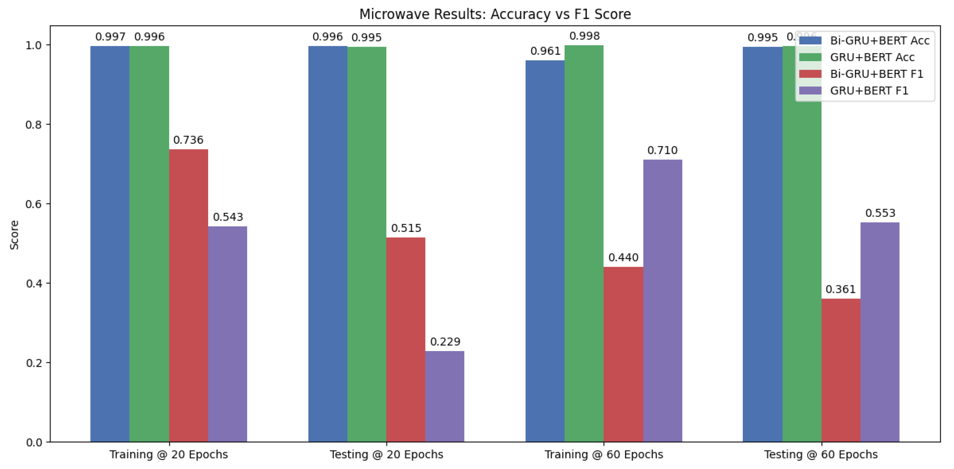
The results on the microwave shown in Table 8 demonstrate that our proposed Bi-GRU+BERT model achieves a test F1-score of 0.515, clearly outperforming BERT4NILM (0.014), ELECTRIcity (0.277), and CTA-BERT (0.209). It also achieves a lower MAE of 5.59 and MRE of 0.013, highlighting its effectiveness in accurately detecting the short and irregular usage patterns of this appliance. However, when trained for 60 epochs, Bi-GRU+BERT exhibits clear signs of overfitting: its test F1-score declines to 0.361 while the MAE increases, despite the training F1-score improving to 0.440. This suggests that the model’s bidirectional recurrence, while helpful for modeling temporal dependencies, may lead to memorization of sparse usage data such as microwave events when exposed to extended training. In contrast, GRU+BERT benefits from its simpler architecture and demonstrates better generalization at 60 epochs, achieving the highest test F1-score of 0.553 and the lowest MAE of 5.24.

The bar chart in Figure 5 illustrates this trend. While Bi-GRU+BERT performs best at 20 epochs, its generalization degrades at 60 epochs. GRU+BERT, on the other hand, shows the opposite behavior with stronger test performance after longer training. This indicates that GRU+BERT can better leverage extended training cycles, whereas Bi-GRU+BERT requires stricter regularization or early stopping to avoid overfitting [31]. This behavior is further supported by the training and validation curves for one training instance shown in Figure 6, where Bi-GRU+BERT’s validation F1-score begins to plateau and then decline after around 20 epochs despite a steady decrease in training loss. This divergence between training and validation performance is a clear sign of overfitting.

Additionally, models like GRU+BERT, BERT4NILM, and ELECTRIcity show signs of overfitting even at early training stages. For example, GRU+BERT achieves a training F1-score of 0.543 at 20 epochs, which already drops to 0.229 on the test set, indicating limited generalization. Similarly, BERT4NILM and ELECTRIcity report high training F1-scores of 0.697 and 0.677, respectively, but their test scores fall to 0.014 and 0.277. This drop is primarily due to the microwave’s infrequent and irregular usage, resulting in very few positive instances during training. As a result, models tend to memorize these limited patterns rather than generalize to unseen data.

The bidirectional GRU layer in our architecture addresses this issue by learning temporal dependencies from both past and future contexts, enabling the model to better capture transient power consumption behaviors. This makes Bi-GRU+BERT, trained for 20 epochs, particularly well-suited for handling the short-duration nature of appliances like microwaves. Figure 7 illustrates this advantage: Figure 7a presents BERT4NILM’s predictions, while Figure 7b shows the output from Bi-GRU+BERT. As is evident, our model generates a more stable and consistent power consumption profile over time, demonstrating its superior generalization capability. Furthermore, Figure 8 provides a zoomed-in view of Bi-GRU+BERT’s predictions, accurately capturing the appliance’s ON/OFF transitions and fine-grained power fluctuations at 20 epochs.

The dishwasher results in Table 9 show that GRU+BERT outperforms Bi-GRU+BERT, achieving F1-scores of 0.777 versus 0.687 at 20 epochs and 0.750 versus 0.688 at 60 epochs. This performance gap suggests that while Bi-GRUs are often beneficial for capturing temporal dependencies, their added complexity may introduce redundancy or noise when modeling appliances with highly structured and sequential multi-phase cycles [31]. Specifically, over-smoothing from bidirectional context can occur because Bi-GRUs combine information from both past and future time steps, which may blur the sharp transitions between operational phases such as wash, rinse, and dry. In such scenarios, the unidirectional GRU appears more effective at preserving the temporal causality needed to track and distinguish operational phases, resulting in better generalization and more reliable event detection.

Lastly, we also report the averaged results in

Table 10. Average test results of all baseline models and our proposed models including the number of training epochs. The best results are highlighted in bold.

Model	Number of Epochs	Accuracy	F1-Score	MRE	MAE (W)
GRU+ (reported from [9])	20	0.789	0.350	0.324	32.25
LSTM+ (reported from [9])	20	0.895	0.304	0.215	24.71
CNN (reported from [9])	20	0.925	0.528	0.188	16.51
BERT4NILM (reported from [7])	20	0.948	0.536	0.167	12.41
BERT4NILM (from our training)	20	0.964	0.552	0.157	13.73
CTA-BERT (reported from [9])	20	0.950	0.595	0.142	11.42
GRU+BERT (proposed)	20	0.970	0.688	0.142	12.11
Bi-GRU+BERT (proposed)	20	0.971	0.728	0.142	13.90
ELECTRIcity (reported from [8])	90	0.963	0.728	0.152	12.15
ELECTRIcity (from our training)	90	0.962	0.700	0.151	12.45
GRU+BERT (proposed)	60	0.971	0.770	0.143	13.01
Bi-GRU+BERT (proposed)	60	0.969	0.712	0.142	12.98

that represent the average of each metric across all five appliances in the test set from Table 5, Table 6, Table 7, Table 8 and Table 9, following the practice adopted by several related works [7,9]. Here, our proposed models demonstrate consistently strong and competitive performance across both short and extended training durations. At 20 epochs, Bi-GRU+BERT achieves the highest average F1-score (0.728) and accuracy (0.971), outperforming all baseline and state-of-the-art models. This highlights the model’s effectiveness in capturing rich temporal dynamics and contextual patterns under limited training.

However, when trained for 60 epochs, GRU+BERT becomes the top performer, achieving the highest average F1-score (0.770) and matching the best accuracy (0.971), while also maintaining competitive error metrics (MRE: 0.143, MAE: 13.01). In contrast, Bi-GRU+BERT shows a slight drop in F1-score (0.712) despite maintaining the lowest average MRE (0.142), suggesting that the added complexity of bidirectional modeling may introduce diminishing returns during extended training. These averaged results confirm that combining GRU-based temporal learning with transformers leads to robust NILM performance, effectively balancing accuracy, generalization, and error reduction across a variety of appliance types and training settings.

Table 11. Comparison of test results between benchmark models and our proposed models on the REDD dataset. N/A in a row means that the corresponding results are not available. The best results are highlighted in bold.

Appliance	Model	Acc.	F1-Score	MRE	MAE (W)
Refrigerator	LSTM+ (reported from [9])	0.789	0.709	0.841	44.82
	GRU+ (reported from [9])	0.794	0.705	0.829	44.28
	CNN (reported from [9])	0.796	0.689	0.822	35.69
	BERT4NILM (reported from [7])	0.841	0.756	0.806	32.35
	CTA-BERT (reported from [9])	0.887	0.761	0.796	30.69
	ELECTRIcity (reported from [8])	N/A	N/A	N/A	N/A
	GRU+BERT (proposed)	0.881	0.801	0.824	32.53
	Bi-GRU+BERT (proposed)	0.858	0.752	0.853	38.194
Microwave	LSTM+ (reported from [9])	0.989	0.604	0.058	17.39
	GRU+ (reported from [9])	0.988	0.574	0.059	17.72
	CNN (reported from [9])	0.986	0.378	0.060	18.59
	BERT4NILM (reported from [7])	0.989	0.476	0.057	17.58
	CTA-BERT (reported from [9])	0.997	0.599	0.056	17.61
	ELECTRIcity (reported from [8])	0.989	0.610	0.057	16.41
	GRU+BERT (proposed)	0.990	0.479	0.069	12.88
	Bi-GRU+BERT (proposed)	0.992	0.646	0.068	12.99
Dishwasher	LSTM+ (reported from [9])	0.956	0.421	0.056	25.25
	GRU+ (reported from [9])	0.955	0.034	0.042	25.29
	CNN (reported from [9])	0.953	0.298	0.053	25.29
	BERT4NILM (reported from [7])	0.969	0.523	0.039	20.49
	CTA-BERT (reported from [9])	0.962	0.472	0.046	22.41
	ELECTRIcity (reported from [8])	0.968	0.601	0.051	24.06
	GRU+BERT (proposed)	0.966	0.503	0.044	23.52
	Bi-GRU+BERT (proposed)	0.960	0.580	0.059	22.93
Average	LSTM+	0.933	0.465	0.244	30.80
	GRU+	0.915	0.382	0.255	28.73
	CNN	0.926	0.410	0.244	28.92
	BERT4NILM	0.948	0.579	0.231	26.35
	CTA-BERT	0.960	0.632	0.229	22.18
	ELECTRIcity	N/A	N/A	N/A	N/A
	GRU+BERT (proposed)	0.947	0.594	0.313	22.98
	Bi-GRU+BERT (proposed)	0.940	0.659	0.327	24.70

presents a comparison of our proposed models against existing benchmark approaches on the REDD dataset. The results show that our GRU+BERT and Bi-GRU+BERT models achieve competitive performance across multiple appliances. For the refrigerator, CTA-BERT achieves the highest accuracy (0.887) and lowest MAE (30.69 W), while GRU+BERT achieves the best F1-score (0.801). On the microwave, Bi-GRU+BERT obtains the highest F1-score (0.646) with low error, whereas CTA-BERT and ELECTRIcity perform best in terms of accuracy and MRE. For the dishwasher, BERT4NILM demonstrates superior accuracy (0.969) and lowest MAE (20.49 W), with Bi-GRU+BERT attaining the highest F1-score (0.580). Averaged across appliances, CTA-BERT consistently provides the best balance of accuracy (0.960), F1-score (0.632), and error metrics, but our GRU-based BERT variants remain competitive, particularly in terms of F1-score and error reduction.

4.4.3. Cross-Dataset Performance Evaluation

In order to assess the generalization ability of our proposed models, we conduct a cross-dataset evaluation by comparing them with BERT4NILM [7]. For fairness, BERT4NILM was run under the same training settings as our models, using the same houses from UK-DALE for training and the same house from REDD for testing.

Table 12. Test results of the three appliances from the REDD dataset after training with the UK-DALE dataset. The best results are highlighted in bold.

Appliance	Model	Accuracy	F1-Score	MAE (W)	MRE
Microwave	BERT4NILM [7]	0.989	0.000	14.03	0.069
	GRU+BERT (proposed)	0.990	0.403	13.70	0.069
	Bi-GRU+BERT (proposed)	0.989	0.328	13.98	0.070
Fridge	BERT4NILM [7]	0.754	0.000	54.26	0.998
	GRU+BERT (proposed)	0.713	0.574	53.67	0.887
	Bi-GRU+BERT (proposed)	0.657	0.542	53.65	0.862
Dishwasher	BERT4NILM [7]	0.459	0.062	42.43	0.554
	GRU+BERT (proposed)	0.946	0.000	29.20	0.050
	Bi-GRU+BERT (proposed)	0.388	0.033	46.99	0.619

presents the cross-dataset evaluation results. For the microwave, both proposed models substantially outperformed the BERT4NILM in terms of F1-score, with GRU+BERT and Bi-GRU+BERT achieving 0.403 and 0.328, respectively, compared to 0.0 from the BERT4NILM. These results demonstrate improved detection of ON/OFF transitions, while MAE and MRE remained nearly identical across all models.

Similarly for the fridge, our proposed models again delivered superior F1-scores (0.574 for GRU+BERT and 0.542 for Bi-GRU+BERT), whereas BERT4NILM failed to detect any events, obtaining an F1-score of 0.0. Although accuracy slightly decreased for the proposed models, the gain in F1-score indicates a stronger capability in capturing appliance state changes. Both proposed variants also reduced the MRE relative to BERT4NILM, reflecting more consistent energy estimation.

In contrast, results were mixed for the dishwasher. The GRU+BERT achieved very high accuracy (0.946) and the lowest MAE (29.20 W) and MRE (0.050), but its F1-score remained 0.0, suggesting difficulty in distinguishing ON/OFF events despite accurate aggregate consumption prediction. The Bi-GRU+BERT, however, underperformed across all metrics, even compared to the BERT4NILM.

These findings are consistent with observations in a recent work by Varanasi et al. [21] where they evaluated cross-dataset performance using the UK-DALE and REFIT datasets for training and REDD for testing. Importantly, they noted that many models attained high accuracies but low F1-scores and even zero scores for certain appliances, e.g., dishwasher, due to very sparse activations in the testing period. This aligns with our findings, where accuracy and MAE can appear strong even when ON/OFF detection, indicated by the F1-score, is weak.

Overall, the cross-dataset results suggest that integrating GRUs with BERT significantly enhances the ability to generalize appliance ON/OFF event detection across unseen datasets, particularly for microwave and fridge. While challenges remain for appliances with sparse or irregular usage patterns, e.g., dishwasher, the proposed models demonstrate stronger robustness compared to BERT4NILM in cross-dataset NILM scenarios.

5. Impact of Architectural Choices and Limitations

In this section, we present ablation studies to better understand the contribution of individual architectural components in our proposed models. Specifically, we examine two design choices: (1) the inclusion of 1D convolutional layers prior to pooling; and (2) the ordering of GRU layers relative to the transformer blocks. By systematically varying these components, we aim to isolate their effects and provide insights into their roles in modeling appliance-level energy consumption across different datasets.

5.1. Effect of Removing the 1D Convolutional Layer

We begin with an analysis of the 1D convolutional layers, which precede pooling in our architectures. To evaluate their importance, we remove them from both the GRU+BERT and Bi-GRU+BERT models and compare the results against the original versions. Since our proposed models achieved the best performance on the microwave and fridge appliances in the UK-DALE dataset, we focus on these appliances to assess the effect of removal of the 1D convolutional layer on the performance.

The results for the fridge from the UK-DALE dataset are shown in Figure 9. It can be observed that the removal of the 1D convolutional layer does not significantly affect the performance. In fact, for Bi-GRU+BERT, the variant without this layer achieved slightly better performance (F1-score of 0.875 vs. 0.871 and lower MRE), while for GRU+BERT, the original model performed marginally better. This suggests that the 1D convolutional layer provides limited benefits for stable load patterns such as the fridge.

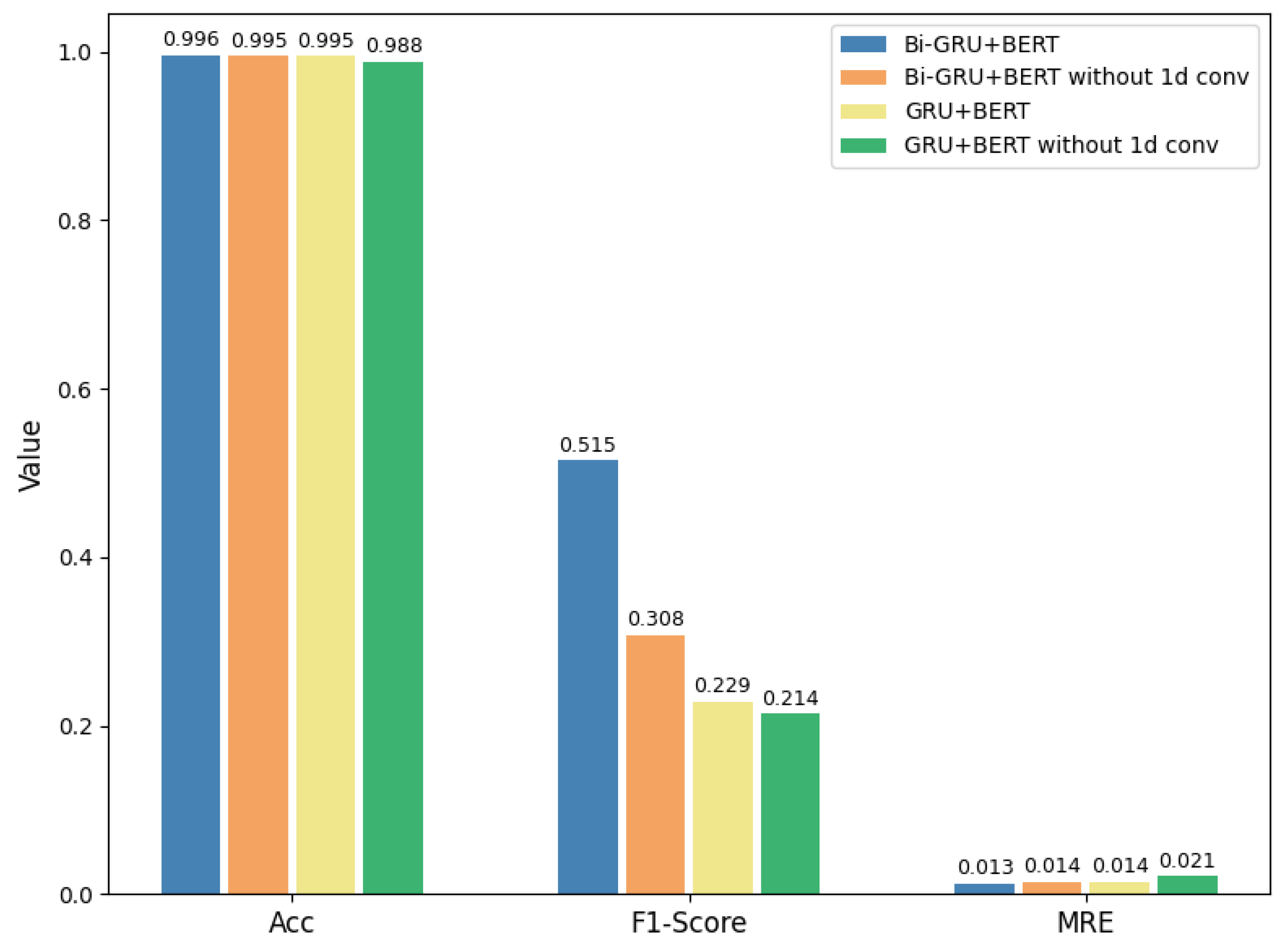
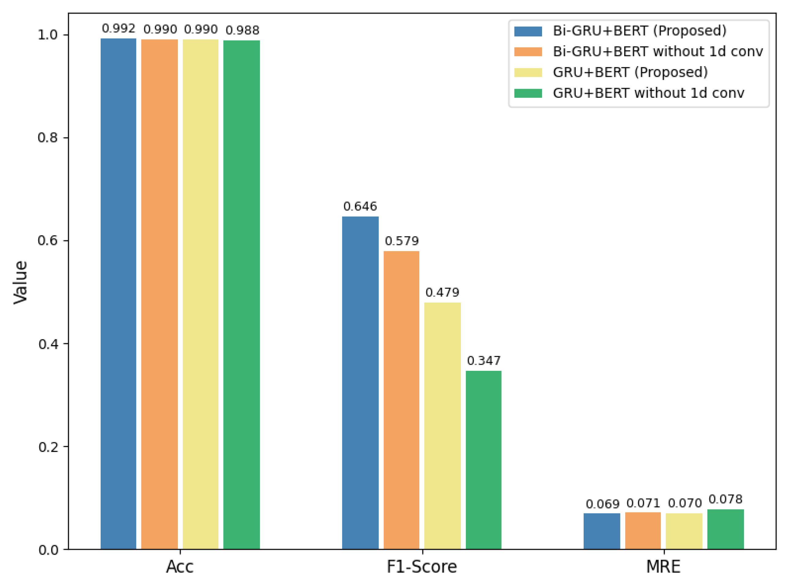
In contrast, for the microwave, as shown in Figure 10, the impact of removing the 1D convolutional layer is considerably more noticeable. While the GRU+BERT model shows a small drop in performance without this layer, the Bi-GRU+BERT model exhibits a substantial decrease in F1-score (from 0.515 to 0.308). This highlights the importance of the 1D convolutional layer in capturing the short, transient usage patterns of appliances like the microwave.

We also show performance differences for fridge and microwave appliances from the REDD dataset in Figure 11 and Figure 12, respectively, where our proposed models perform better than the variants that have no 1D convolutional layers. Based on these observations, we retained the 1D convolutional layer in our proposed architectures to ensure consistent performance across different appliance types and datasets.

5.2. Positioning GRU Layers Relative to Transformer Blocks

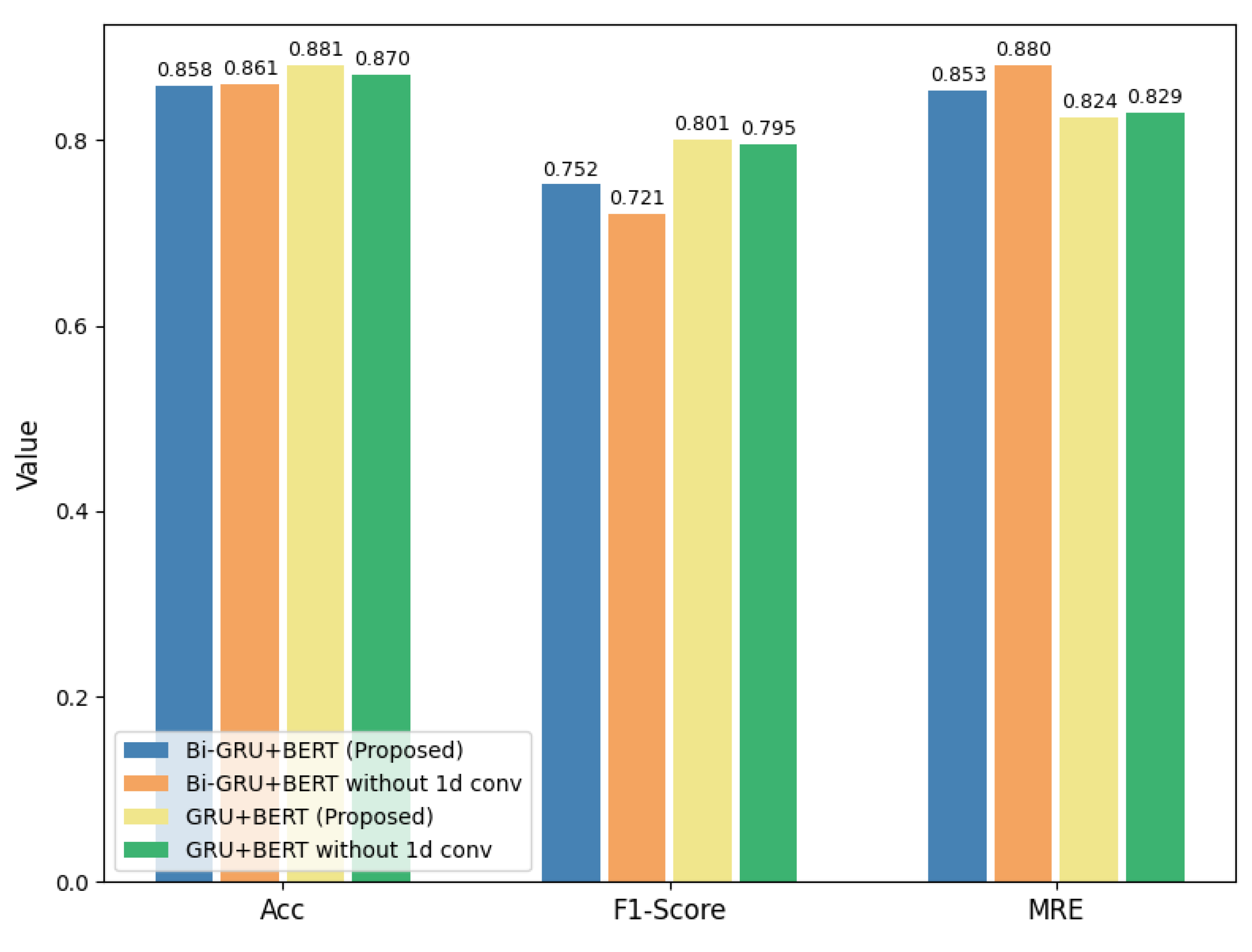
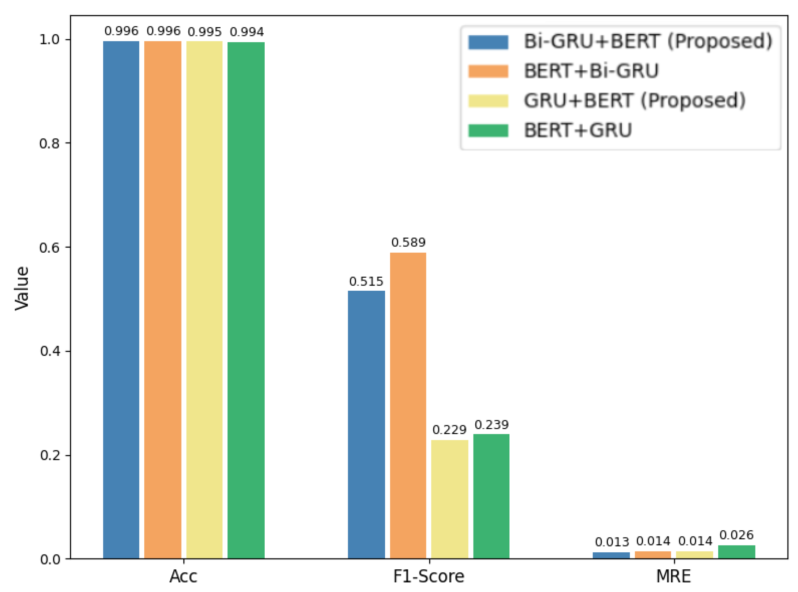
We further experiment with our models by interchanging the position of the GRU/Bi-GRU layers and BERT. Specifically, we compare our proposed architectures where the GRU layers are placed before the transformer blocks as shown in Figure 2, with variants where these recurrent layers are positioned after the transformer blocks. We denote these interchanged variants as BERT+GRU and BERT+Bi-GRU in Figure 13 and Figure 14, presenting the performance comparison on the UK-DALE dataset for the fridge and microwave appliances, respectively.

The results obtained on the UK-DALE dataset indicate that moving the GRU layers after the transformer blocks leads to marginal improvements. For the fridge, Bi-GRU+BERT with reordered components achieved a slightly higher F1-score (0.873 vs. 0.871). Similarly, for the microwave, Bi-GRU+BERT improved notably from 0.515 to 0.589, showing that this arrangement helps capture transient load signatures more effectively. The GRU+BERT model showed mixed outcomes: while it improved slightly on the microwave (0.229 vs. 0.239), it performed worse on the fridge (0.871 vs. 0.858).

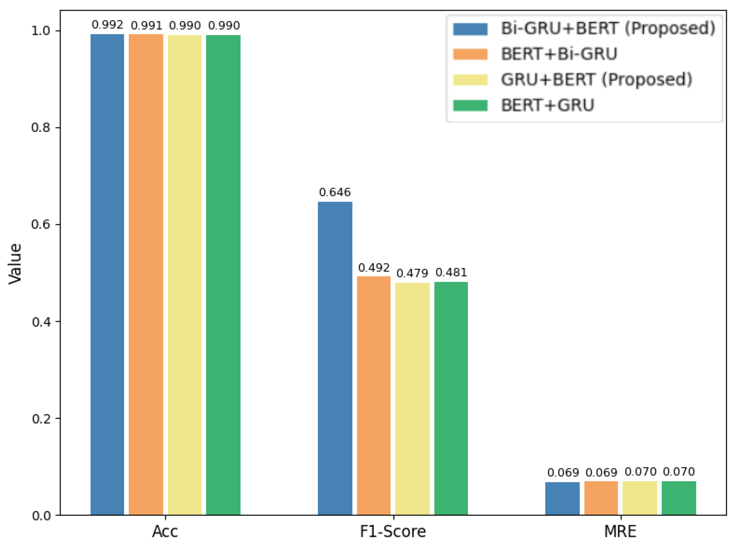
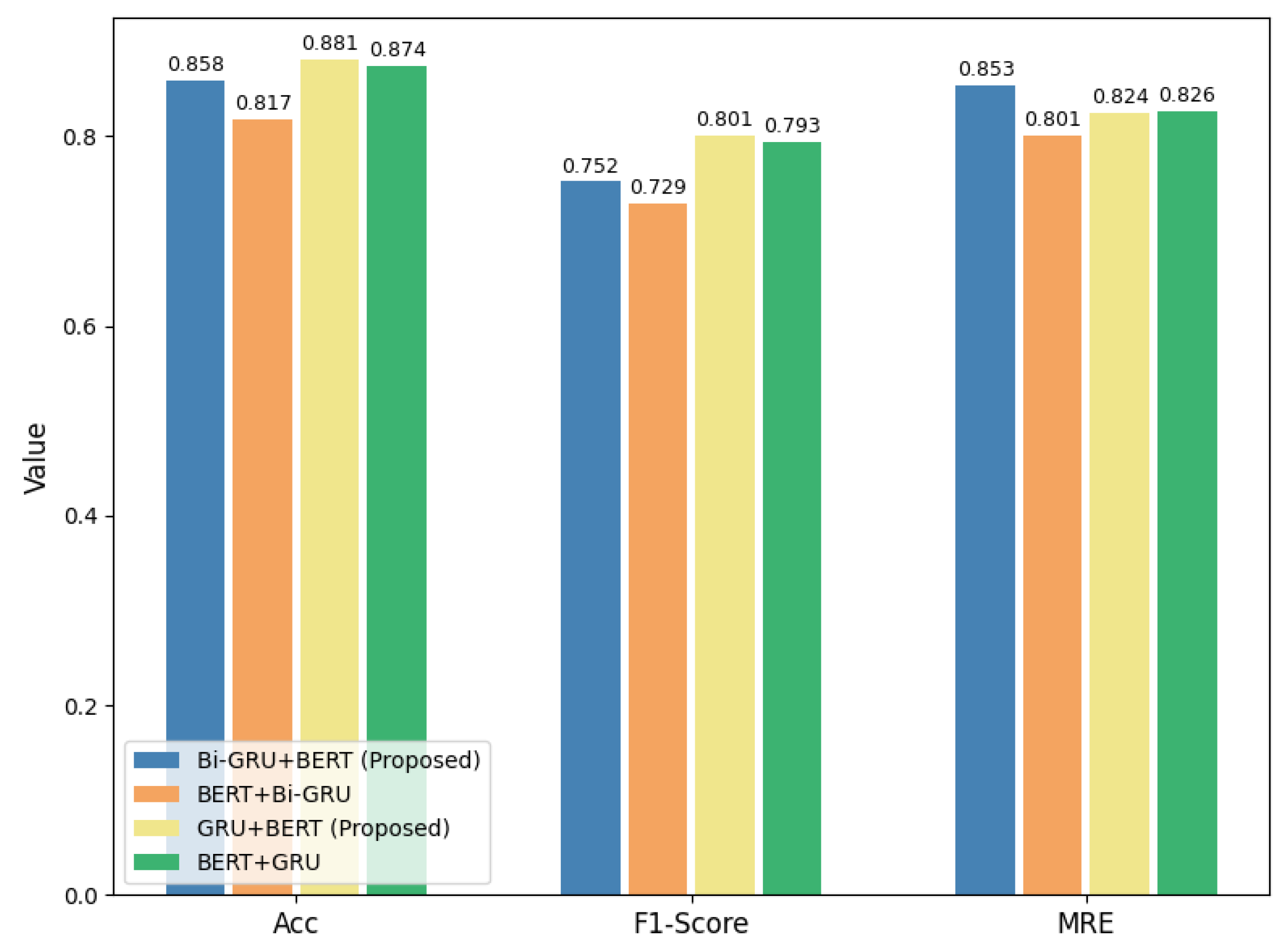
However, when tested on the REDD dataset, the opposite trends were observed. Figure 15 and Figure 16 show the comparative performance on the microwave and fridge, respectively. For the former, Bi-GRU+BERT’s F1-score dropped from 0.646 to 0.492 after reordering, and GRU+BERT showed no meaningful improvement (0.479 vs. 0.481). For the fridge, both models also exhibit performance degradation, with Bi-GRU+BERT’s performance deteriorating from 0.752 to 0.729 and that of GRU+BERT dropping from 0.801 to 0.793.

Overall, these experiments suggest that the optimal placement of GRU layers is dataset-dependent. On the UK-DALE dataset, positioning the GRU layers after the transformer blocks provides some benefits, particularly for appliances with transient signals such as the microwave. In contrast, on the REDD dataset, retaining the original design (GRU layers before the transformer blocks) yields consistently better and more stable results across different appliances. Therefore, we adopt our proposed architecture with GRU layers preceding the transformer blocks as the more reliable configuration.

5.3. Model Limitations and Future Extensions

The proposed models in this work are currently designed for single-appliance prediction, which allows direct comparison with existing state-of-the-art baselines. This design does not directly support multi-appliance disaggregation. Architecturally, the models could be extended to handle multiple appliances simultaneously by incorporating multi-output prediction layers and leveraging multi-task learning, representing a promising direction to improve scalability and practical applicability of NILM systems.

Future work includes several directions. On the architectural side, enhancements such as causal GRUs with limited look-ahead, phase-aware attention mechanisms, and alternative attention modules, e.g., gated attention, sparse/local attention, or the Temporal Fusion Transformer, could better capture temporal dependencies, improve prediction accuracy, and explore trade-offs between computational efficiency and real-time applicability. While full cross-house k-fold evaluation and bootstrapped statistical tests are computationally intensive, they remain valuable avenues for strengthening model assessment.

From a deployment perspective, we plan to investigate practical integration with smart home systems, real-time edge/cloud implementation, and household-specific personalization to account for unique appliance usage patterns. To mitigate overfitting on sparse appliances such as microwaves, strategies such as class reweighting, synthetic data generation, data augmentation, curriculum learning, and appliance-specific transient-aware loss functions will be explored. Additionally, techniques such as model pruning or quantization could reduce resource requirements, enabling potential on-device deployment while maintaining strong performance.

6. Conclusions

In this paper, we proposed a hybrid deep learning architecture that integrated GRUs with a transformer-based BERT encoder to enhance the NILM performance. By combining local temporal modeling and global contextual attention, our approach addressed key limitations of existing models, which often struggle with disaggregation of appliances that exhibit short, transient, or complex usage patterns. We developed two variants, GRU+BERT and Bi-GRU+BERT, each showing distinct strengths at different training regimes. Specifically, the Bi-GRU+BERT model outperformed both the GRU+BERT and existing state-of-the-art models when trained for 20 epochs. However, when the training was extended to 60 epochs, the simpler GRU+BERT model demonstrated superior performance, outperforming the Bi-GRU+BERT model and maintaining stability across appliances, especially those with sparse activation. Precisely, our experimental results demonstrate clear improvements over the nearest baselines. For the fridge, both GRU+BERT and Bi-GRU+BERT achieved an F1-score of 0.871, compared to 0.801 for the best-performing BERT4NILM baseline. This performance corresponds to an absolute improvement of 0.070 and a relative gain of approximately 8.7%. For the microwave, GRU+BERT attained an F1-score of 0.553 (trained for 60 epochs) with Bi-GRU+BERT reaching an F1-score of 0.515 (trained for 20 epochs). The proposed models substantially outperformed the best-performing CNN baseline at 0.341, representing absolute improvements of 0.212 and 0.174 and relative gains of 62% and 51%, respectively. For the washing machine, GRU+BERT and Bi-GRU+BERT achieved F1-scores of 0.877 and 0.857, respectively, compared to 0.835 for the best-performing baseline ELECTRIcity model, yielding absolute improvements of 0.042 and 0.022 or relative gains of approximately 5% and 2.6%, respectively. These results highlight the complementary strengths of the two models, with Bi-GRU+BERT excelling under constrained training settings and GRU+BERT offering more stable performance with prolonged training.

References

1. Zhang, C.; Zhong, M.; Wang, Z.; Goddard, N.; Sutton, C. Sequence-to-point learning with neural networks for non-intrusive load monitoring. In Proceedings of the AAAI Conference on Artificial Intelligence, New Orleans, LA, USA, 2–7 February 2018; Volume 32. [Google Scholar]
2. Batra, N.; Kelly, J.; Parson, O.; Dutta, H.; Knottenbelt, W.; Rogers, A.; Singh, A.; Srivastava, M. NILMTK: An open source toolkit for non-intrusive load monitoring. In Proceedings of the 5th International Conference on Future Energy Systems, Cambridge, UK, 11–13 June 2014; pp. 265–276. [Google Scholar]
3. Rafiq, H.; Zhang, H.; Li, H.; Ochani, M.K. Regularized LSTM based deep learning model: First step towards real-time non-intrusive load monitoring. In Proceedings of the 2018 IEEE International Conference on Smart Energy Grid Engineering (SEGE), Oshawa, ON, Canada, 12–15 August 2018; pp. 234–239. [Google Scholar]
4. Kolter, J.Z.; Jaakkola, T. Approximate inference in additive factorial hmms with application to energy disaggregation. In Proceedings of the Artificial Intelligence and Statistics, PMLR, La Palma, Spain, 21–23 April 2012; pp. 1472–1482. [Google Scholar]
5. Mauch, L.; Yang, B. A novel DNN-HMM-based approach for extracting single loads from aggregate power signals. In Proceedings of the 2016 IEEE International Conference on Acoustics, Speech and Signal Processing (ICASSP), Shanghai, China, 20–25 March 2016; pp. 2384–2388. [Google Scholar]
6. Schirmer, P.A.; Mporas, I. Non-intrusive load monitoring: A review. IEEE Trans. Smart Grid 2022, 14, 769–784. [Google Scholar] [CrossRef]
7. Yue, Z.; Witzig, C.R.; Jorde, D.; Jacobsen, H.A. Bert4nilm: A bidirectional transformer model for non-intrusive load monitoring. In Proceedings of the 5th International Workshop on Non-Intrusive Load Monitoring, Virtual, 18 November 2020; pp. 89–93. [Google Scholar]
8. Sykiotis, S.; Kaselimi, M.; Doulamis, A.; Doulamis, N. Electricity: An efficient transformer for non-intrusive load monitoring. Sensors 2022, 22, 2926. [Google Scholar] [CrossRef] [PubMed]
9. Xuan, Y.; Pang, C.; Yu, H.; Zeng, X.; Chen, Y. Load energy decomposition algorithm based on improved bidirectional transformer combined with time-sensing self-attention. IEEE Access 2024, 12, 75625–75639. [Google Scholar] [CrossRef]
10. Ciancetta, F.; Bucci, G.; Fiorucci, E.; Mari, S.; Fioravanti, A. A new convolutional neural network-based system for NILM applications. IEEE Trans. Instrum. Meas. 2020, 70, 1–12. [Google Scholar] [CrossRef]
11. Wang, L.; Mao, S.; Nelms, R.M. Transformer for nonintrusive load monitoring: Complexity reduction and transferability. IEEE Internet Things J. 2022, 9, 18987–18997. [Google Scholar] [CrossRef]
12. Sun, C.; Huang, L.; Qiu, X. Utilizing BERT for aspect-based sentiment analysis via constructing auxiliary sentence. arXiv 2019, arXiv:1903.09588. [Google Scholar] [CrossRef]
13. Yao, S.; Bi, J. Sentiment Analysis Based on the BERT and Bidirectional GRU Model. In Proceedings of the 2024 IEEE 7th International Conference on Information Systems and Computer Aided Education (ICISCAE), Dalian, China, 27–29 September 2024; pp. 290–295. [Google Scholar]
14. Zhang, X.; Wu, Z.; Liu, K.; Zhao, Z.; Wang, J.; Wu, C. Text sentiment classification based on BERT embedding and sliced multi-head self-attention Bi-GRU. Sensors 2023, 23, 1481. [Google Scholar] [CrossRef] [PubMed]
15. Makhmudov, F.; Kultimuratov, A.; Cho, Y.I. Enhancing Multimodal Emotion Recognition through Attention Mechanisms in BERT and CNN Architectures. Appl. Sci. 2024, 14, 4199. [Google Scholar] [CrossRef]
16. Lee, J.; Yoon, W.; Kim, S.; Kim, D.; Kim, S.; So, C.H.; Kang, J. BioBERT: A pre-trained biomedical language representation model for biomedical text mining. Bioinformatics 2020, 36, 1234–1240. [Google Scholar] [CrossRef] [PubMed]
17. Khodeir, N.A. Bi-GRU urgent classification for MOOC discussion forums based on BERT. IEEE Access 2021, 9, 58243–58255. [Google Scholar] [CrossRef]
18. Hung, B.T. Document classification by using hybrid deep learning approach. In Proceedings of the International Conference on Context-Aware Systems and Applications, My Tho City, Vietnam, 28–29 November 2019; pp. 167–177. [Google Scholar]
19. Zhang, H.; Liu, Y.; Qiu, Y.; Liu, H.; Pei, Z.; Wang, J.; Long, M. Timesbert: A bert-style foundation model for time series understanding. arXiv 2025, arXiv:2502.21245. [Google Scholar]
20. Devlin, J.; Chang, M.W.; Lee, K.; Toutanova, K. Bert: Pre-training of deep bidirectional transformers for language understanding. In Proceedings of the 2019 Conference of the North American Chapter of the Association for Computational Linguistics: Human Language Technologies, Volume 1 (Long and Short Papers), Minneapolis, MN, USA, 2–7 June 2019; pp. 4171–4186. [Google Scholar]
21. Varanasi, L.S.; Karri, S.P.K. STNILM: Switch Transformer based Non-Intrusive Load Monitoring for short and long duration appliances. Sustain. Energy Grids Netw. 2024, 37, 101246. [Google Scholar] [CrossRef]
22. Kelly, J.; Knottenbelt, W. The UK-DALE dataset, domestic appliance-level electricity demand and whole-house demand from five UK homes. Sci. Data 2015, 2, 1–14. [Google Scholar] [CrossRef] [PubMed]
23. Kolter, J.Z.; Johnson, M.J. REDD: A public data set for energy disaggregation research. In Proceedings of the Workshop on Data Mining Applications in Sustainability (SIGKDD), San Diego, CA, USA, 21–24 August 2011; Volume 25, pp. 59–62. [Google Scholar]
24. Angelis, G.F.; Timplalexis, C.; Krinidis, S.; Ioannidis, D.; Tzovaras, D. NILM applications: Literature review of learning approaches, recent developments and challenges. Energy Build. 2022, 261, 111951. [Google Scholar] [CrossRef]
25. García, D.; Pérez, D.; Papapetrou, P.; Díaz, I.; Cuadrado, A.A.; Enguita, J.M.; Domínguez, M. Conditioned fully convolutional denoising autoencoder for multi-target NILM. Neural Comput. Appl. 2025, 37, 10491–10505. [Google Scholar] [CrossRef]
26. Rahman, M.; Arafat, Y. Towards a deeper understanding of transformer for residential non-intrusive load monitoring. In Proceedings of the 2024 International Conference on Innovations in Science, Engineering and Technology (ICISET), Chittagong, Bangladesh, 26–27 October 2024; pp. 1–6. [Google Scholar]
27. Mekruksavanich, S.; Jitpattanakul, A. Hybrid convolution neural network with channel attention mechanism for sensor-based human activity recognition. Sci. Rep. 2023, 13, 12067. [Google Scholar] [CrossRef] [PubMed]
28. Ylla, I. Non-Intrusive Load Disaggregation (Energy-Disaggregation-DL). 2021. Available online: https://github.com/inesylla/energy-disaggregation-DL (accessed on 31 August 2025).
29. Neyshabur, B.; Sedghi, H.; Zhang, C. What is being transferred in transfer learning? Adv. Neural Inf. Process. Syst. 2020, 33, 512–523. [Google Scholar]
30. Tsaptsinos, D.; Leigh, J. Modelling of a fermentation process using Multi-Layer Perceptrons: Epochs vs Pattern learning, Sigmoid vs Linear transfer function. J. Microcomput. Appl. 1993, 16, 125–136. [Google Scholar] [CrossRef]
31. Wang, X.; Xie, G.; Zhang, Y.; Liu, H.; Zhou, L.; Liu, W.; Gao, Y. The Application of a BiGRU Model with Transformer-Based Error Correction in Deformation Prediction for Bridge SHM. Buildings 2025, 15, 542. [Google Scholar] [CrossRef]
Figure 1. Basic illustration of our model input–output flow.
Ai 06 00238 g001
Figure 2. Detailed architecture of the Bi-GRU+BERT model that takes a fixed length of sequential data and outputs the disaggregated power prediction with the same temporal resolution.
Ai 06 00238 g002
Figure 3. Performance metrics (validation accuracy, F1-score and relative error, and training loss) of the fridge using Bi-GRU+BERT model over 60 training epochs.
Ai 06 00238 g003
Figure 4. Prediction of fridge power consumption with ON/OFF states using the Bi-GRU+BERT model. An ON/OFF threshold of 50 W is used to determine appliance state.
Ai 06 00238 g004
Figure 5. Comparison of training and test results for GRU+BERT and Bi-GRU+BERT models at 20 and 60 epochs. Each group of bars contrasts the two models for both training and testing, with accuracy and F1-scores shown side by side. The figure highlights that while GRU+BERT benefits from extended training to 60 epochs, Bi-GRU+BERT overfits beyond 20 epochs, confirming that earlier training provides the most stable performance for this appliance.
Ai 06 00238 g005
Figure 6. Training and validation performance of Bi-GRU+BERT on the microwave. The plots show the training loss, validation relative error, validation accuracy, and validation F1-score across 60 epochs. While training loss continues to decrease, the validation F1-score peaks around 20 epochs and then declines, indicating overfitting when training is extended beyond this point.
Ai 06 00238 g006
Figure 7. Comparison of microwave power consumption prediction between (a) BERT4NILM and (b) Bi-GRU+BERT.
Ai 06 00238 g007
Figure 8. Zoomed-in view of microwave power consumption prediction using the Bi-GRU+BERT model, highlighting the model’s accuracy in tracking ON/OFF states and transient behaviors. As the microwave usage is typically sparse with short, high-power bursts, only selected data points where the appliance was active are shown to illustrate prediction fidelity during actual operation. An ON/OFF threshold of 200 W is used to determine the appliance state.
Ai 06 00238 g008
Figure 9. Ablation results for the fridge appliance on the UK-DALE dataset, showing the effect of removing the 1D convolutional layer from the proposed models.
Ai 06 00238 g009
Figure 10. Ablation results for the microwave appliance on the UK-DALE dataset, showing the effect of removing the 1D convolutional layer from the proposed models.
Ai 06 00238 g010
Figure 11. Ablation results for the fridge appliance on the REDD dataset, showing the effect of removing the 1D convolutional layer from the proposed models.
Ai 06 00238 g011
Figure 12. Ablation results for the microwave appliance on the REDD dataset, showing the effect of removing the 1D convolutional layer from the proposed models.
Ai 06 00238 g012
Figure 13. Ablation results for the fridge appliance on the UK-DALE dataset, showing the impact of reordering the GRU layers relative to the transformer blocks in the proposed models.
Ai 06 00238 g013
Figure 14. Ablation results for the microwave appliance on the UK-DALE dataset, showing the impact of reordering the GRU layers relative to the transformer blocks in the proposed models.
Ai 06 00238 g014
Figure 15. Ablation results for the microwave appliance on the REDD dataset, showing the impact of reordering the GRU layers relative to the transformer blocks in the proposed models.
Ai 06 00238 g015
Figure 16. Ablation results for the fridge appliance on the REDD dataset, showing the impact of reordering the GRU layers relative to the transformer blocks in the proposed models.
Ai 06 00238 g016