Article

Improving Remote Access Trojans Detection: A Comprehensive Approach Using Machine Learning and Hybrid Feature Engineering

by
AlsharifHasan Mohamad Aburbeian
1,
Manuel Fernández-Veiga
2 and
Ahmad Hasasneh
3,*
1
Doctoral Program in Information and Communications Technologies (DocTIC), Universidade de Vigo, 36310 Vigo, Spain
2
AtlanTTic Research Center, Universidade de Vigo, 36310 Vigo, Spain
3
Faculty of Artificial Intelligence, Arab American University, Ramallah P600, Palestine
*
Author to whom correspondence should be addressed.
AI 2025, 6(9), 237; https://doi.org/10.3390/ai6090237
Submission received: 12 August 2025 / Revised: 18 September 2025 / Accepted: 19 September 2025 / Published: 21 September 2025

Abstract

Remote Access Trojans (RATs) pose a serious cybersecurity risk due to their stealthy control over compromised systems. This study presents a detection framework that integrates host, network, and newly engineered behavioral features to enhance the identification of RATs. Two sets of experiments were performed: (i) using the original dataset only, and (ii) using an extended dataset with ten engineered features and importance analysis. The framework was evaluated on a public Kaggle dataset of an RAT and benign traffic. Eight machine learning classifiers were tested, including three baseline methods, four ensemble approaches, and a neural network. Results show that the engineered hybrid feature set substantially improves detection performance. Among the tested algorithms, Random Forest and MLP achieved the strongest performance, with accuracies of 98% and 97%, respectively, while Gradient Boosting and LightGBM also performed competitively. Performance was assessed using multiple metrics, and to gain deeper insight into model learning behavior, learning curves and Precision–Recall curves were analyzed. The results demonstrate how well hybrid feature modeling, neural networks, and ensemble machine learning techniques may improve RAT identification. In future work, exploring the use of explainable ML methods may improve the detection capabilities.

1. Introduction

1.1. Background

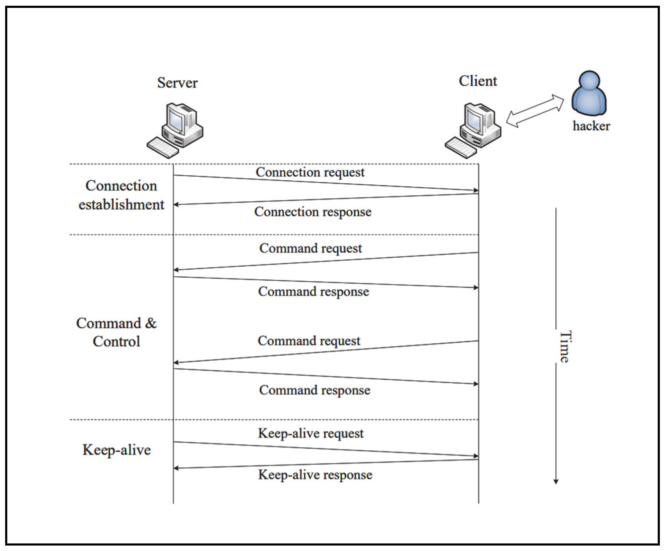
The malicious malware Remote Access Trojan (RAT) enables intruders to remotely take control of systems and intercept data, having a significant negative impact on governments, businesses, and private citizens [1]. The RAT is generally made up of an infected side and a control side. To discover the computers that can be infected, attackers can employ phishing, social engineering, or any other techniques to deliver the RAT into the victim’s device [2]. To prevent their appearance on the task list, concealment methods integrate themselves into other legal processes in which the RAT operations become more similar to those of legitimate programs, and it becomes harder to identify RATs. RATs typically rely on a client/server design. The attacker controls the client device to either directly steal information from the target device or employ the remote control ability of the target host by using the client to manage the server [3]. Figure 1 shows the runtime states of the RAT, which are connection setup, keep-alive, and command and control.
As shown in Figure 1, the connection establishment phase is the first and shortest stage in a RAT’s lifecycle, during which the attacker delivers the RAT and establishes the initial connection. After that, the system alternates between two recurring states: keep-alive and command-and-control [4]. The keep-alive state lasts the longest and involves minimal activity. During this phase, the RAT server sends small periodic signals (keep-alive requests) to check whether the client is still connected. These packets are typically tiny and contain little information [5]. From a detection standpoint, this quiet behavior can be identified by analyzing the network packets and monitoring the limited number of host operations. In contrast, the command-and-control state is more active and involves frequent communication between the client and server. Once connected, the attacker can issue commands to the client, which are executed by the server. This state often involves large data transfers, especially when the attacker is stealing sensitive information [6]. Finally, because of its malicious action, which was discussed previously, RAT becomes a serious problem in cyberspace [7]. This research presents a methodology for detecting RATs by employing various machine learning algorithms to achieve the highest possible accuracy.
Figure 1. Different operational states of a Remote Access Trojan (RAT) [5].
Ai 06 00237 g001

1.2. Related Studies

Through the literature, numerous studies have discussed RAT detection, and the different methodologies used by other researchers can be categorized into three groups: host-based, network-based, and hybrid-based. This section will discuss each one separately.

1.2.1. Host-Based Studies

The host-based approach relies on evaluating and monitoring the behavior of RATs as they run on infected devices. To identify and detect RATs, they use various metrics based on execution data from the operating system, such as CPU and memory utilization [8], processor execution path [9], process ID, and API requests [10]. According to Moon et al. [11], the system behavior of a typical software may be used to identify malware from an Advanced Persistent Threat (APT) attack. A technique for spotting APT malware that focuses on “changes” in host behavior was implemented by Chandran et al. [12]. It utilizes data such as CPU and memory utilization, system files, and open ports. Using the communication and processing data, Liang et al. [13] suggested a method for logging suspicious communications from Trojans. This host-based approach relies on studies of static analysis techniques based on syntactic signatures or semantic properties. However, identifying a Trojan using only the static analysis technique may not be effective [14]. Moreover, malware that employs code obfuscation methods is challenging to examine using this method [15]. A deep learning method for RAT detection was introduced by Floroiu et al. [16]. Their method utilized an image classification model and converted executable files into grayscale texture images. The deployment dataset was constructed using both benign samples and files infected by known RATs. At 83.26%, they had the highest accuracy score among multiple deep learning models. However, the model’s ability to identify RATs is constrained by its dependence on session-level variables and low accuracy. Their findings also indicate that addressing the unbalanced dataset is necessary to improve identification.

1.2.2. Network-Based Studies

RATs are often detected using network recognition methods by examining the network traffic’s payload, examining the behavior of their users, or examining their statistical properties. To characterize the activity of the RAT, Li et al. [17] utilized four IP-level characteristics: the quantity of incoming and outgoing packets, the length of the communication session, the number of transport layer connections, and a couple of flow-level characteristics: packet delivery time and packet time interval. Their model’s false positive rate (FPR) is less than 3.2%, while the accuracy is over 91%. However, this may still allow sensitive data to be exposed before the threat is detected, due to delayed identification. Liang et al. [13] described the behavior of Trojans using five typical characteristics, which are the active connection percentage, the number of unique IPs, the ratio of transmitted to received traffic size, the uploaded connection percentage, and the number of connections. The FPR was 2.94%, with an accuracy of 97.05%. It can be hard to identify Trojans as quickly as possible, and the precise quantity of benign and Trojan cases was not mentioned in the study. In the early stages of TCP communication, RAT traffic can be identified, as achieved by Jiang et al. [18]. This study used 175 sessions for detection purposes. Only 10 RAT sessions were used and 165 benign ones. Their Random Forest classifier accuracy was 96%, and the FPR was 10%. An unbalanced distribution of Trojan and benign sessions was also deployed in other studies [19,20]. This makes the deployed classifier unable to distinguish between Trojan and benign traffic correctly. Sebakara et al. [21] introduced a model for RAT identification in their study. The model is based on metadata and behavioral signs at the network level, including persistent unidirectional flows, irregularities in TLS handshakes, and anomalies in packet timing. Several classifiers were trained and assessed. The Random Forest performed the best, with a 72.11% accuracy. However, their methodology was less dependable when detecting RATs because it is solely static and vulnerable to obfuscation strategies, and it requires further improvements for better detection.

1.2.3. Hybrid-Based Studies

In this approach, the characteristics of both the host and network features are combined to describe the behavior of the RATs. For example, an approach to identifying RAT-Bots was introduced by Awad et al. [22]. They suggested a framework that involves two stages that work together to detect RAT bots early on. The first stage depends on the host-based behavior, which monitors the host’s system activity and raises an alert in the event of any irregularities. The second stage relies on network-based behavior, monitoring network traffic, and identifying any suspicious trends. This strategy significantly depends on the host agent since the network agent does not start operating until the host agent sends the alarm. Guo et al. [5] proposed a system that combines both host and network characteristics to detect RATs. To increase the True Positive Rate (TPR) in their model, they trained two distinct recognition models, each tailored to a particular RAT operational stage. However, their data were highly skewed (benign: 28,730 records; Trojan: 251 records), which would lead to unreliable model accuracy due to the bias towards the benign category [23,24]. Another strategy was put forth to identify RATs in an LAN environment by employing a range of static and dynamic analysis techniques [25]. Both host-level activity analysis (using Process Explorer and static inspection tools like VirusTotal) and network traffic analysis (using Wireshark) are integrated in this work. The detection framework monitors the compromised host and examines the traffic it produces, spanning both ends of the RAT communication channel. Their method lacks machine learning approaches and does not evaluate performance under network variability, latency, or detection accuracy.
Despite the significant advancements in host-based, network-based, and hybrid RAT detection methods, several limitations remain unaddressed in the current literature. Many host-based studies rely heavily on static analysis techniques, which are often ineffective against obfuscated or polymorphic malware and may lack the context of external communication patterns. Network-based approaches usually rely on limited session-level features and struggle with high false positive rates or delayed detection, particularly when encountering encrypted or stealthy communication. Moreover, several prior studies suffer from highly imbalanced datasets, which compromise classifier reliability by biasing detection toward benign instances. Hybrid approaches have shown promise, but existing models often lack rich behavioral feature sets or rely on sequential triggers between host and network agents, limiting their responsiveness and detection scope [5]. To overcome these issues, this study suggests a hybrid detection methodology that combines a balanced dataset and advanced feature engineering.
The main contributions of this study are as follows:
  • Hybrid detection approach: A novel framework is proposed that combines host-based and network-based features to enhance RAT detection.
  • Improved accuracy and lower false positives: By integrating various features, the approach enhances classification accuracy and reduces false alarms.
  • Broader threat coverage: The hybrid method captures both external network behaviors (e.g., command-and-control activity) and internal host indicators (e.g., unauthorized access attempts).
  • Highlighting the significance of feature engineering: The study introduces and evaluates 10 newly engineered behavioral features that significantly improve model performance.

2. Materials and Methods

2.1. Methodology

This study introduces a new machine learning method for detecting RATs by combining host and network features. Two models were created: Model A, which includes the original dataset features along with engineered behavioral features, and Model B, which uses only the original dataset features without the added engineered attributes. This setup enabled a systematic evaluation of how feature engineering impacts the performance of RAT detection. The methodology used in this research is illustrated in Figure 2.
As illustrated in Figure 2, the study approach contains six main stages, beginning with data acquisition and followed by feature engineering and data preprocessing. The final stages focus on enhancing and evaluating the performance using several metrics. To ensure robust performance, the study employed a diverse set of algorithms, including Logistic Regression (LR), Naive Bayes (NB), K-nearest neighbors (KNN), Random Forest (RF), Gradient Boosting (GB), AdaBoost, LightGBM, and Multilayer Perceptron (MLP).
Linear models such as Logistic Regression provide interpretability and computational efficiency, making them suitable for establishing baseline performance. Naive Bayes is effective in high-dimensional spaces under conditional independence assumptions. Instance-based methods like K-Nearest Neighbors leverage local similarity and lazy learning, enabling direct comparisons between flow instances. Ensemble tree-based methods further enhance predictive power: Random Forest captures complex feature interactions and reduces variance through bagging, Gradient Boosting sequentially corrects errors from prior trees to improve accuracy, AdaBoost iteratively reweights misclassified samples to focus on challenging instances, and LightGBM optimizes leaf-wise growth for the efficient handling of large, high-dimensional datasets. Finally, MLP, as a neural network, learns intricate nonlinear patterns and hierarchical representations in the data.
By combining these diverse classifiers, the study ensures that different aspects of RAT behavior are captured and that conclusions are not biased toward any single algorithmic assumption. This comprehensive evaluation enables the identification of the most effective models for RAT detection and provides robust insight into the benefits of hybrid feature engineering.

2.2. Data Acquisition

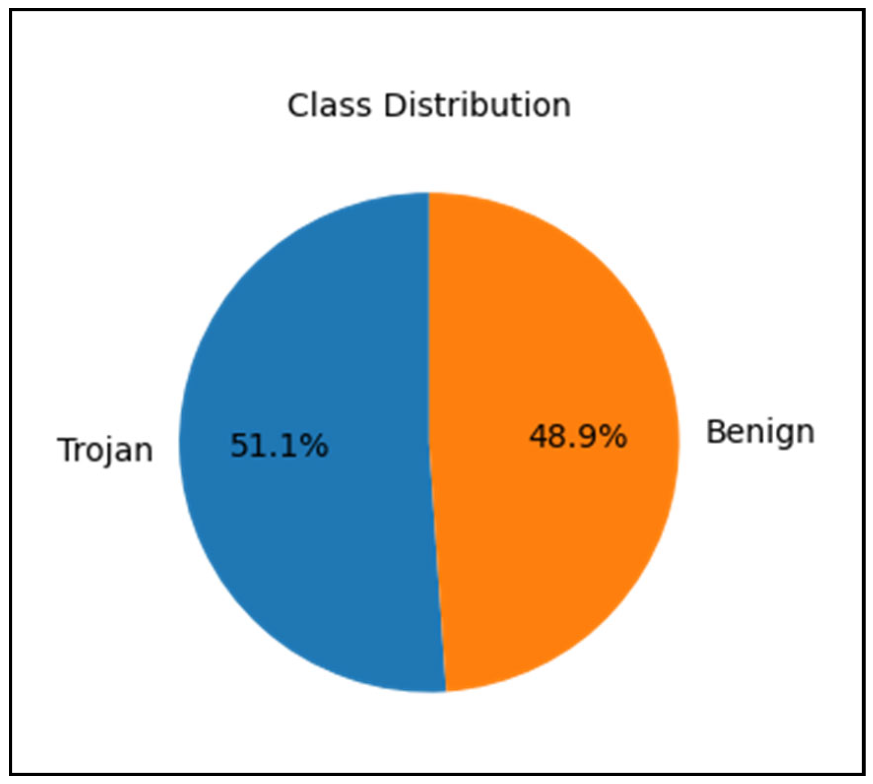
The dataset used in this study was generated by the “Canadian Institute for Cybersecurity (CIC)” and downloaded from the Kaggle website [26]. It includes 177,482 network traffic records, each representing a flow instance labeled as either benign or a RAT. The dataset distribution is shown in Figure 3.
As shown in Figure 3, the dataset is roughly balanced, with 86,799 benign instances and 90,683 RAT instances, offering a nearly even class distribution. This balance reduces the need for extensive rebalancing initially, leading to more reliable training and evaluation of classification models. Although this study used a balanced and publicly available Kaggle dataset for training and assessment, such a distribution might not accurately reflect real-world RAT traffic, where benign flows are much more common. While this balancing was necessary to reduce classifier bias, it also introduces a limitation in terms of realism.

2.3. Feature Engineering

Feature engineering is essential for improving performance. It entails generating, altering, or choosing critical characteristics in unprocessed data to enhance the machine learning model’s efficiency [27]. In security-related tasks such as malware and RAT detection, the raw features in the original dataset capture low-level traffic statistics. By deriving additional behavioral features, we can reveal deeper patterns of activity that better distinguish malicious from benign behavior. This study introduced 10 new features that capture time-based, interaction-based, and behavioral characteristics of network flows. These features help reveal insights such as flow intensity, temporal activity, frequency of communication, and the diversity of contacts between IP addresses. Table 1 below summarizes the engineered features, their source features, and their classification, and provides a brief description of each one.
As shown in Table 1, the newly introduced features include time-related attributes such as “Hour, DayOfWeek, IsWeekend, and SecondsSinceMidnight”, which capture temporal patterns that can reveal attack timing behavior. Behavioral network features, such as “TimeDiffFromLastFlow, SourceIP_FlowCount, UniqueDestinations, and UniqueSources”, offer critical insights into how a source or destination behaves across connections, helping to identify anomalies like port scanning, lateral movement, or unusual communication volume. The “AvgFlowDuration” captures how long a source typically communicates in a session, which may further distinguish malicious flows.
To measure their impact, ablation experiments were performed: model A (hybrid without engineered features) and model B (hybrid with engineered features).

2.4. Data Cleaning and Preprocessing

To ensure data readiness, a comprehensive data preprocessing procedure was implemented. Initially, the preprocessing pipeline for Model A included removing non-informative features such as the “FlowID, and Unnamed: 0” index column, which was a CSV-generated identifier without analytical value. The “Timestamp, and FlowDate” columns were excluded to reduce redundancy and potential information leakage, as their identifying information had already been encoded into more meaningful derived features during the feature engineering phase. Categorical fields such as “Source IP, Destination IP, and Protocol” were transformed into numerical representations; specifically, the IP addresses were hashed into integers to preserve anonymity and maintain compatibility with machine learning algorithms, while the protocol values were encoded using categorical codes. The target variable “Class”, labeled initially with the string values “Benign” and “Trojan”, was mapped to binary numeric values (0 and 1, respectively) for classifier compatibility. To ensure data quality, all columns were assessed for missing values; any rows containing invalid timestamps had already been removed during earlier parsing steps. A final verification step confirmed that no missing values remained. Furthermore, all remaining features were verified to be numeric, aligning the dataset with the input requirements of the selected machine learning frameworks.
Model B followed the same preprocessing pipeline as Model A. Non-informative columns such as “FlowID” and “Unnamed: 0” were removed, categorical fields were transformed into numerical representations, IP addresses were hashed into integers, protocol values were encoded, and the target variable was mapped to binary numeric values (0 and 1). The only difference is that no derived behavioral features were added, and no feature importance or selection was performed
These steps collectively ensured the dataset was clean, numerically consistent, and free from features that could hinder the learning process.

2.5. Feature Selection

To improve performance and reduce computational load, this study employed a comprehensive feature selection and importance analysis process. Not all features contributed equally to classifying benign and RAT traffic. To identify the most critical features, a Random Forest classifier was trained on the preprocessed data. This model was chosen because of its ability to rank features based on their effectiveness in reducing impurity in decision trees. The feature importance was then assessed and ranked. A threshold of 0.001 was applied to exclude features that had minimal impact on the model’s decisions. Refer to Table 2, which lists the features and their descriptions after the feature importance analysis.
As shown in Table 2, the analysis revealed that several engineered behavioral features, such as “DayOfWeek, SecondsSinceMidnight, and IsWeekend” were among the most influential, highlighting the significance of temporal patterns in RAT detection. Network-based metrics such as SourceIP_FlowCount, UniqueDestinations, Flow Duration, and packet statistics like “Flow Bytes/s, Fwd IAT Max, and Packet Length Variance” also showed strong importance scores. In contrast, features like “RST Flag Count, Fwd URG Flags, ECE Flag Count”, and several bulk transfer indicators had an importance of zero and were thus removed.
Out of the ten engineered features, nine were retained in the final set of seventy after applying feature importance analysis. Features such as “FlowDate” were excluded to avoid redundancy; however, they were primarily used as intermediate variables to derive more meaningful features like “DayOfWeek” and “IsWeekend”, which were retained. Similarly, the identifiers feature “FlowID” and the “Timestamp” feature were removed, while their temporal information was already captured in other derived features. Thus, the final feature set preserves the essential behavioral signals introduced by our feature engineering, while avoiding redundant or less informative variables.
To facilitate the reader’s understanding of the final number of features, Figure 4 shows the roadmap for the feature engineering process.
As shown in Figure 4, Model A starts with 86 features. Ten features were extracted through feature engineering, as illustrated previously in Table 1. Four features were dropped, as discussed in Section 2.4. Finally, 22 features were dropped according to importance analysis. As a result, the final number of features in Model A is 70 features, including the label (Trojan, benign). The retained set included a mix of original network features, derived behavioral features, and key host indicators that were empirically validated to contribute significantly to the classification task. This selective pruning of the feature space not only improved training efficiency but also helped mitigate overfitting, as the models were now trained on the most informative subset of data. Model B has 86 features too; 2 features were dropped as discussed previously in Section 2.4. As a result, the final number of features in Model A is 70 features, including the label (Trojan, benign).

2.6. Data Splitting and Model Preparation

To prepare the dataset for training and evaluation, stratified sampling was used to split it into 80% for training and 20% for testing. The distribution was nearly balanced, with Trojan samples forming a slight majority. The training set maintained a class balance of approximately 49% benign and 51% Trojan, while the testing set preserved the same ratio. To address the slight imbalance in the training data and enhance the distinguishability of both classes, the Synthetic Minority Over-sampling Technique (SMOTE) was applied. To prevent data leakage, the dataset was first split into training and testing sets. Then, SMOTE was applied only to the training set to balance the classes before model fitting. The same data splitting process was used for both models. SMOTE generates synthetic data for the minority class, resulting in a perfectly balanced training set with 50% for each class. Table 3 summarizes the distribution of class labels across training, testing, and SMOTE-balanced training sets.
As Table 3 shows, the whole dataset consisted of 177,482 rows, which were divided into 141,985 rows (80%) for training and 35,497 rows (20%) for testing. The training set included 69,439 benign and 72,546 Trojan records, while the testing set contained 17,360 benign and 18,137 Trojan records. After applying SMOTE, the balanced training set consisted of 72,546 samples for each class, totaling 145,092 rows.
Finally, with the dataset preprocessed, features selected, and class distribution balanced, both models were ready for testing the machine learning algorithms. The following section presents the experimental results.

3. Results

3.1. Experiments

3.1.1. Hardware and Software Configuration

This study’s experiments were performed utilizing the “Python programming language within the Anaconda Jupyter Notebook environment (version 3)”. All code was executed on a standard “personal computer equipped with an Intel® Core™ (Santa Clara, CA, USA) i5-10210U CPU @ 1.60GHz (2.11 GHz), 16 GB of RAM”, with Windows 11 Pro OS.
All experiments were implemented in Python (version 3.9.12). The primary libraries included scikit-learn (version 1.0.2), LightGBM (version 4.6.0), NumPy (version 1.21.5), Pandas (version 1.4.2), Matplotlib (version 3.5.1), and Seaborn (version 0.11.2). This setup provided sufficient computational resources for model training, hyperparameter tuning, and visualization. The primary objective was to create a trustworthy and interpretable framework capable of accurately detecting and classifying RAT traffic.

3.1.2. Classifier Design and Tuning

To improve detection performance, specific enhancements were applied to each classifier for both models. The Logistic Regression model was trained on standardized features with L2 regularization (C = 1.0) and a maximum of 3000 iterations to ensure convergence. For Naive Bayes, the 25 most informative features were selected and scaled before training, with the var_smoothing parameter tuned from 10−9 to 10−5 for stable probability estimation. The K-Nearest Neighbors classifier was optimized by testing k values of 3, 5, and 7 with uniform and distance-based weights, while scaling the input features to ensure meaningful distance comparisons.
The ensemble and neural models were also configured with tailored enhancements. The Random Forest model was trained with 200 estimators, meaning it constructed 200 independent decision trees and aggregated their predictions through majority voting, which improves stability and reduces variance. The trees were allowed to grow fully (no maximum depth) to capture complex patterns, while parallel execution (n_jobs = −1) optimized training efficiency. The Gradient Boosting classifier also employed 200 estimators, but in contrast to RF, these were built sequentially, where each tree corrected the mistakes of the previous one. The learning rate of 0.05 reduced the weight of each tree’s contribution for smoother convergence, while the maximum depth of 3 limited tree complexity to prevent overfitting. Stochasticity was introduced with a subsample ratio of 0.8, where each tree was trained on 80% of the samples, improving generalization. The AdaBoost model used 100 estimators, representing 100 weak learners (shallow trees), each reweighted to emphasize previously misclassified samples, allowing the ensemble to iteratively improve its focus on difficult-to-detect Trojans. Similarly, the LightGBM model was configured with 100 estimators and a learning rate of 0.05 but optimized for efficiency by using a maximum depth of 5 and 31 leaves per tree, which constrained memory usage while preserving predictive power. Finally, the MLP neural network was designed with two hidden layers, each containing 128 and 64 neurons, respectively, allowing it to learn hierarchical representations of traffic patterns. It was trained with a maximum of 500 iterations, with early stopping to prevent overfitting, and regularization was applied through an L2 penalty (alpha = 0.0005).
To ensure reproducibility, a fixed random seed (random_state = 42) was applied during train–test splitting, SMOTE balancing, and in classifiers that support seed initialization (Random Forest, Gradient Boosting, AdaBoost, Logistic Regression, and LightGBM). For deterministic classifiers such as k-Nearest Neighbors and Naïve Bayes, reproducibility is inherent. For the MLPClassifier, results may vary slightly due to weight initialization when no random seed is specified.
Together, these models represent a diverse mix of simple, ensemble learning, and deep neural approaches, ensuring both interpretability and adaptability in detecting RAT activity.

3.1.3. Ablation Experiments

To rigorously evaluate the impact of feature engineering, two models were developed. Model B was trained using only the original dataset features, whereas Model A extended this feature space with ten newly engineered behavioral attributes. Both models were trained and tested under identical conditions to ensure a fair and unbiased comparison.
A consistent preprocessing pipeline was applied to both models, including data cleaning, normalization, the handling of missing values, and the use of SMOTE to balance the training set. Each model was then evaluated with the same set of eight classifiers: three simple algorithms, four ensemble methods, and one neural network. For each classifier, the relevant pipeline components (as described in Section 2.4) were integrated to ensure consistency and prevent bias across the experiments.

3.2. Metrics and Results

Demonstrating accuracy through testing alone is not enough to prove the algorithm’s reliability. Therefore, the results were evaluated using various metrics, including the confusion matrix, classification report, ROC curves, precision–recall curves, learning curves, and model training time. Each metric will be explained and discussed in separate sections. For Model A, all these metrics will be shown to provide a thorough assessment of its performance. Conversely, Model B results will be presented using only the classification report, as this highlights the effect of feature engineering without needing a complete comparative analysis.

3.2.1. Confusion Matrix

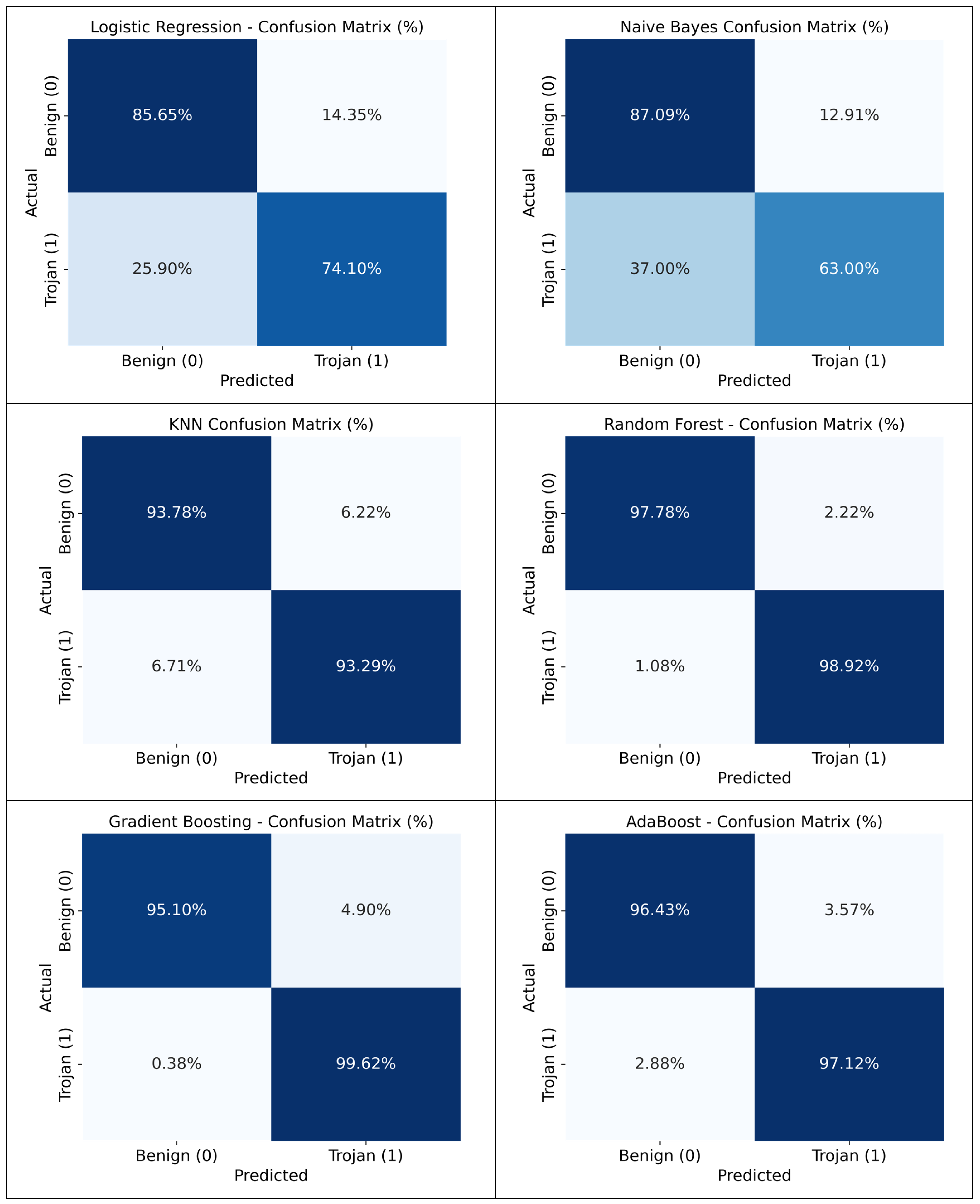
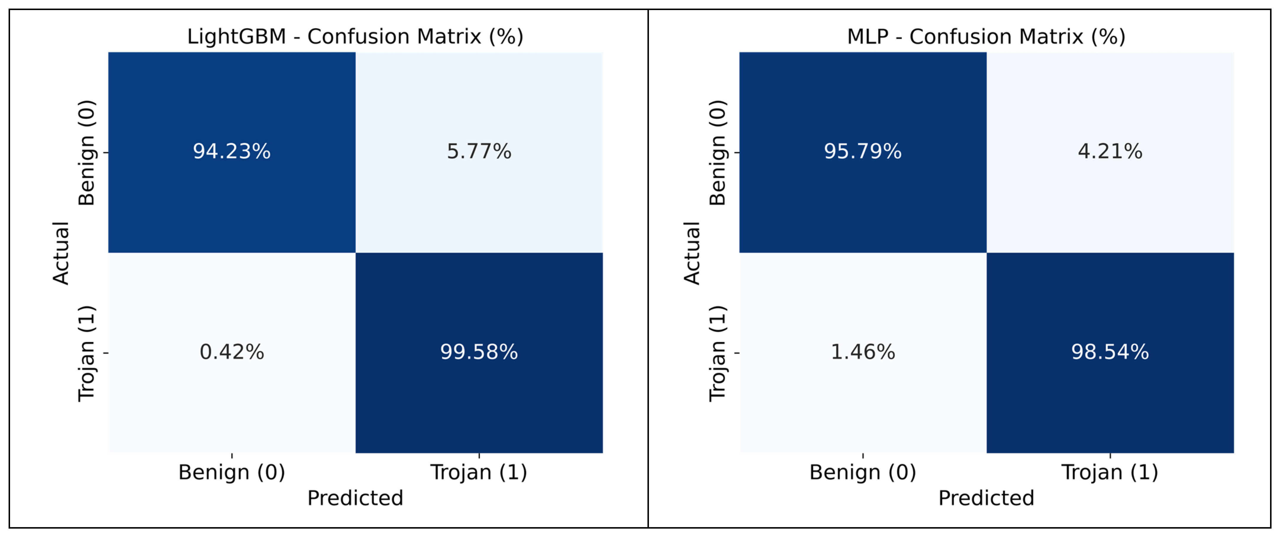
The confusion matrix is a method for classification problems that shows how well a model performs by breaking down correct and incorrect predictions for each class. It divides predictions into four categories: True Positives (TP), True Negatives (TN), False Positives (FP), and False Negatives (FN). TP indicates that your model correctly predicted a positive outcome. TN indicates a correct negative prediction. FP refers to a positive prediction that was incorrect. FN refers to a negative prediction that was wrong [28]. This metric enables a detailed analysis of how effectively each class is identified. The results of the confusion matrix are shown in Figure 5.
As shown in Figure 5, the Logistic Regression correctly predicted 86% of benign flows and 74% of Trojan flows. The Naïve Bayes classifier achieved 87.17% accuracy for benign traffic and 64.17% for Trojan traffic. In contrast, the Random Forest classifier correctly predicted 98% of benign samples and 99% of Trojan samples. The Gradient Boosting, AdaBoost, LightGBM, and MLP models were able to predict the Trojan traffic with accuracies of 99.62%, 97.12%, 99.58%, and 98.54%, respectively.

3.2.2. The Classification Report

Accuracy, precision, recall, and F1 score measures are the outcome of the classification report. The fraction of correctly anticipated results is known as the accuracy. By multiplying the overall quantity of predictions by the sum of TPs and TNs, the classifier’s overall accuracy can be determined. Although accuracy is frequently the best criterion to assess a classifier’s effectiveness. However, for a more thorough comprehension of the classifier’s functionality, various measures should be considered [29]. The quantity of properly recognized outputs is used to calculate precision. Recall is the proportion of TPs, while the F1 score is the average of precision and recall [30]. Table 4 displays the results of the classification report for Model A, and Table 5 shows the results for Model B.
Table 4 reports that Logistic Regression, Naïve Bayes, and k-Nearest Neighbors algorithms achieved accuracies of 80%, 75%, and 94%, respectively. Both Random Forest and Gradient Boosting algorithms obtained 98% accuracy, while AdaBoost, LightGBM, and MLP classifiers achieved an accuracy of 97%.
Table 5 shows that Logistic Regression, Naïve Bayes, and k-Nearest Neighbors achieved accuracies of 50%, 52%, and 54%, respectively. The highest results were for the Random Forest classifier, with an accuracy of 81% and precision and recall values of 85% and 77% for the Trojan class. The classifiers Gradient Boosting, AdaBoost, LightGBM, and MLP achieved accuracies of 74%, 73%, 76%, and 75%, respectively.

3.2.3. ROC Curve

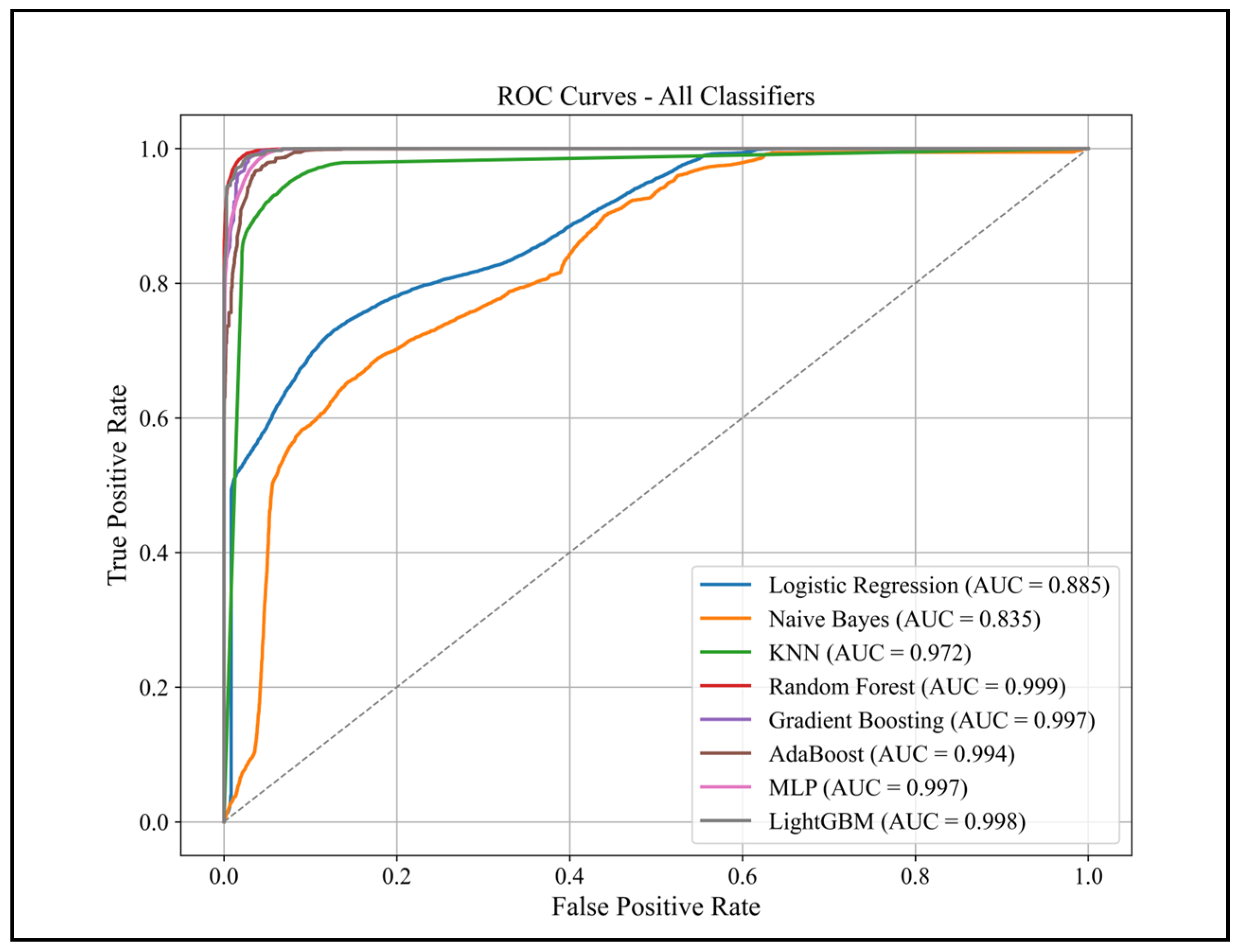
The Receiver Operating Characteristic (ROC) curve is a visualization used to assess a binary classifier’s effectiveness. It demonstrates the connection between the TP rate and the FP rate over various categorization levels [31]. Figure 6 presents the ROC curve results.
As seen in Figure 6, the ensemble and MLP algorithms exhibit curves that closely approach the upper-left corner. In contrast, Logistic Regression and Naïve Bayes had ROC curves closer to the diagonal.

3.2.4. Precision–Recall Curves

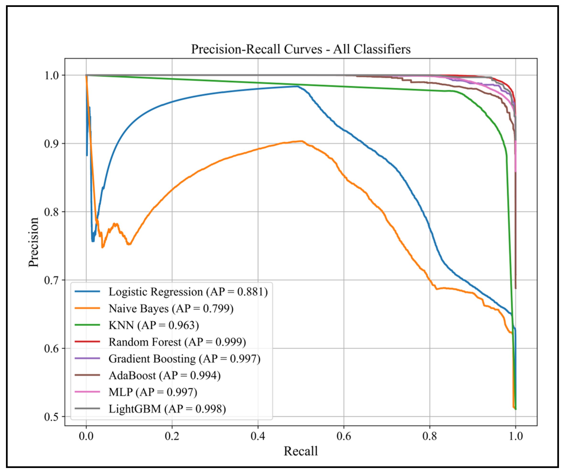
The Precision–Recall (PR) curve is a diagnostic tool that focuses on the performance of a classifier concerning the positive class (Trojan traffic) [32]. The curve displays precision against recall at various threshold values. PR curves are exceptionally informative when dealing with imbalanced datasets, as they provide more meaningful insight than ROC curves when the positive class is rare. Figure 7 shows the PR curves for the same set of models evaluated in the ROC curve analysis.
According to Figure 7, the ensemble and MLP algorithms consistently achieved high precision and recall across thresholds, with higher average precision scores than Logistic Regression and Naïve Bayes.

3.2.5. Learning Curve and Training Time Results

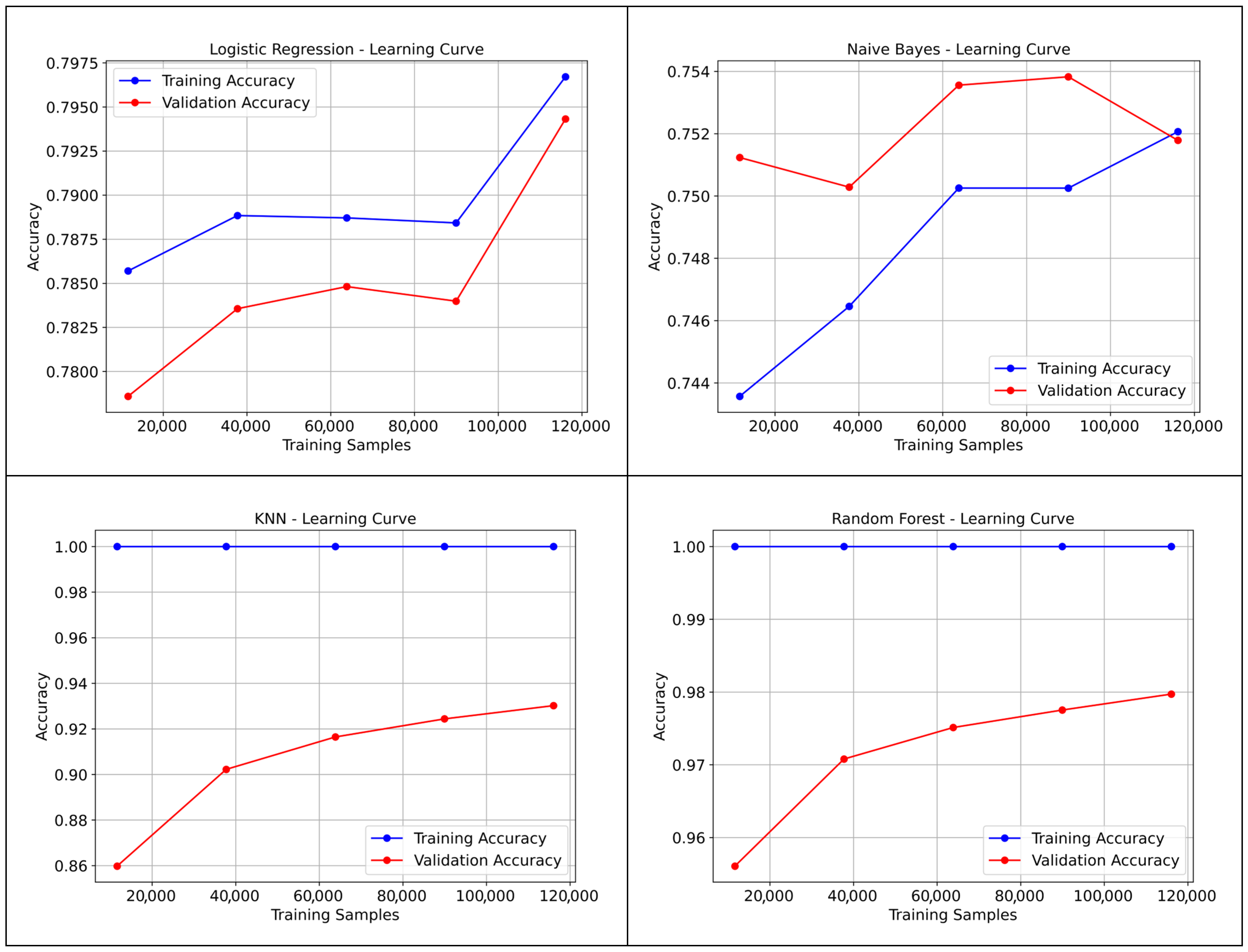
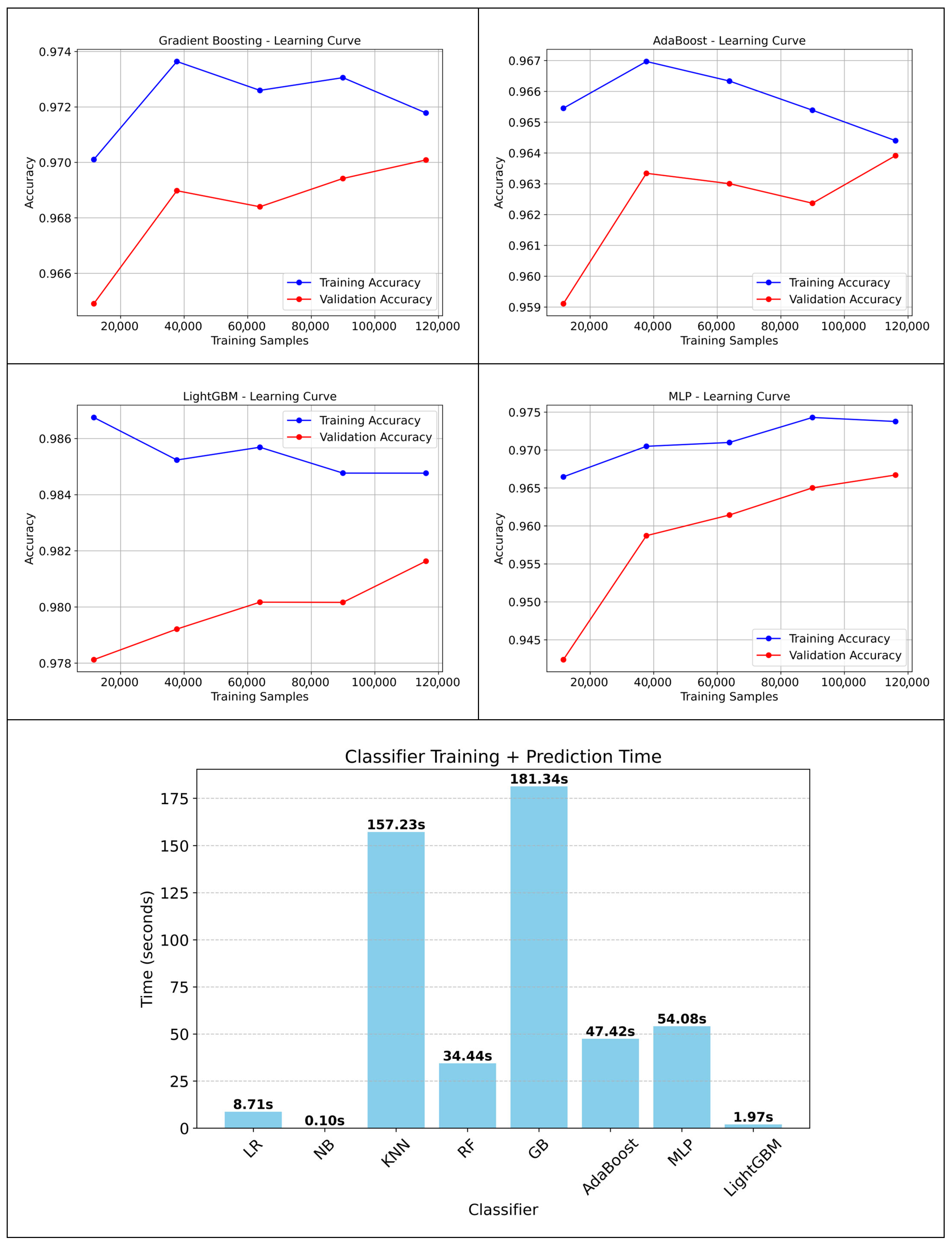
A learning curve illustrates how a model’s performance evolves with increasing training set size [33]. It provides details on how effectively the model generalizes and whether it suffers from underfitting or overfitting. In contrast, the training time bar chart in the bottom-right corner quantifies the computational cost required to fit each model to the whole training dataset. Figure 8 presents a comprehensive analysis of model behavior using both learning curves and a training time comparison.
As shown in Figure 8, Random Forest and Gradient Boosting demonstrated steadily increasing validation accuracy as training data increased, closely following their training accuracy. AdaBoost and LightGBM also showed consistent performance, with validation curves staying near their training curves across all data sizes. The MLPClassifier consistently had a small gap between training and validation accuracy. Logistic Regression reached early convergence, with nearly identical training and validation curves, while Naïve Bayes displayed more variation in validation accuracy. K-Nearest Neighbors maintained high training accuracy, with validation improving gradually as the data size expanded. The training times in seconds were LightGBM (1.79 s), Logistic Regression (8.71 s), Naïve Bayes (0.10 s), k-Nearest Neighbors (157.23 s), Random Forest (34.44 s), Gradient Boosting (181.34 s), AdaBoost (47.42 s), and MLP (50.08 s).

3.2.6. Inference Performance

Inference performance measures how efficiently a trained model can make predictions using new data, considering factors such as latency, memory usage, and CPU utilization. Table 6 provides a comparison of Model A in terms of these metrics.
As shown in Table 6, Logistic Regression exhibited memory usage of ≈1616 MB and CPU utilization of 101.9%. K-Nearest Neighbors required higher memory (≈1695 MB) and CPU (157.1%), with an average latency per sample of 1.986 milliseconds (MS). Random Forest, Gradient Boosting, and AdaBoost consumed between 1690 and 1703 MB of memory, with CPU utilization ranging from 96.2% to 100.2%, and latency per sample from 0.0022 to 0.0154 MS. LightGBM used 1645.98 MB of memory with a CPU utilization of 180.3% and 0.0024 MS latency per sample. The MLP classifier showed the highest CPU usage at 380.6%, memory of 1703.42 MB, and latency of 0.0020 MS per sample.

3.2.7. Feature Contribution Analysis for Ensemble ML Methods

As discussed in Section 3.1.2, all classifiers were carefully tuned using optimal hyperparameters to achieve the best performance while minimizing the risk of overfitting. To gain deeper insights into the contribution of each feature in the predictive process, an importance analysis was conducted specifically for the ensemble algorithms, including Random Forest, Gradient Boosting, AdaBoost, and LightGBM. This analysis highlights which features most strongly influence the model’s decisions and provides an understanding of the relative weight of each attribute in detecting RAT behavior. Figure 9 shows the analysis results.
As shown in Figure 9, “DayOfWeek” and “SecondsSinceMidnight” were the most significant features across all classifiers. For Random Forest, the most important features were “IsWeekend, Hour, and Source IP”. For Gradient Boosting, the top features included “Source IP, SourceIP_FlowCount, and UniqueSources”. The AdaBoost model highlighted “Source IP, Destination IP, and SourceIP_FlowCount”, while LightGBM identified “Source IP, Destination IP, and Flow Packets” as the key contributors.

4. Discussion

The evaluation results show that ensemble and neural network methods are more effective for RAT detection than linear or probabilistic classifiers. For example, Random Forest and MLP have demonstrated the ability to achieve high detection rates for both benign and malicious categories. This advantage is due to their capacity to model complex, nonlinear relationships between features.
The performance gap between advanced and simpler models is also clear in the ROC and Precision–Recall analyses. Ensemble classifiers, especially Random Forest and Gradient Boosting, generated nearly perfect ROC curves while maintaining high precision even at higher recall levels. Likewise, MLP demonstrated a strong balance between precision and recall, highlighting its robustness against false positives. In contrast, Logistic Regression and Naïve Bayes performed poorly when recall increased, revealing their limitations in scenarios that require maximum detection coverage.
Learning curve patterns further validated these findings. Random Forest and Gradient Boosting showed consistent improvements with more training data, while MLP maintained solid generalization with only a small training–validation gap. AdaBoost and LightGBM also displayed strong consistency, thanks to their boosting frameworks. Conversely, K-Nearest Neighbors was sensitive to variance and improved more slowly, Logistic Regression plateaued early due to bias issues, and Naïve Bayes remained unstable because of its independence assumption.
Training time comparisons show a trade-off between predictive performance and computational efficiency. While Random Forest, Gradient Boosting, AdaBoost, and MLP take longer to train, their higher accuracy may justify the extra cost in high-security situations. On the other hand, Naïve Bayes and Logistic Regression run faster but have lower detection ability. The performance evaluation of the classifiers highlights notable differences in memory usage, CPU utilization, and inference latency. Most models, including Logistic Regression and Naive Bayes, have moderate memory footprints around 1.6–1.7 GB, while tree-based models such as Random Forest, Gradient Boosting, AdaBoost, and MLP slightly exceed 1.7 GB. K-Nearest Neighbors, LightGBM, and MLP exhibit higher memory demands, reflecting the need to store extensive data structures during inference. CPU utilization varies considerably: simpler models like Logistic Regression and Naive Bayes remain close to 100%, whereas K-Nearest Neighbors, LightGBM, and especially MLP exceed 150–380%, indicating parallel processing or multi-core usage during computation. Latency per sample is minimal for most models (<0.003 MS), except for K-Nearest Neighbors, which incurs a much higher cost (≈1.99 MS) due to its instance-based computation. Overall, these results suggest that while more complex models may provide higher predictive capacity, they also require significantly more computational resources, which should be considered when deploying them in resource-constrained environments.
Ablation experiments further underscored the importance of feature engineering. Using the new behavioral features, Model A consistently outperformed Model B across all classifiers. These features significantly boosted neural network and ensemble classifiers, showing that behavioral patterns can distinguish RAT traffic. As detailed in Section 3.2.6, most of the top-ranked features were engineered attributes, confirming that the newly created behavioral features significantly contributed to the improved detection performance. To compare the study results, Table 7 presents the results of some related studies that used the same ML algorithms to address the RAT issue.
As shown in Table 7, some earlier studies reported higher KNN accuracy than ours [18,37]; however, our approach achieved better results with ensemble methods such as Random Forest, Gradient Boosting, AdaBoost, and LightGBM. The very high results reported for Random Forest (up to 99.7% [36] and 100% [39]) may suggest overfitting, particularly since these studies lack robustness checks. Additionally, most related works only present accuracy, without comprehensive evaluation metrics, and seldom include class distribution details, making it hard to determine whether their models are biased toward the majority class. In contrast, our study provides a complete set of performance metrics, explicitly analyzes both classes, and validates results across multiple classifiers. Our results do not conflict with previous malware detection research [25,39,40,41,42,43,44]. This study confirms that combining hybrid feature design with well-tuned machine learning models can significantly improve RAT detection efficiency.
False positives remain one of the toughest challenges when deploying RAT detection systems in real-world settings. In high-risk industries like healthcare, finance, and critical infrastructure, even a small FP rate can have serious consequences. For instance, in hospitals, unnecessary alarms might divert analysts’ attention from actual threats to electronic medical records; in financial companies, too many false alerts can interfere with fraud detection and delay responses to incidents; and in industrial control systems, harmless flows that are mistakenly identified as malicious can lead to costly service disruptions or shutdowns. These examples demonstrate that high precision is not only desirable but also essential for practical deployment.
From an operational standpoint, the study demonstrates that hybrid feature integration provides a practical and effective basis for real-world intrusion detection systems. The engineered behavioral features, particularly those that capture temporal patterns and connection diversity, directly relate to common RAT tactics, such as persistence, scheduled execution, and lateral movement. By increasing sensitivity to these behaviors, the framework enhances resilience against stealthy techniques that often evade traditional signature-based defenses. Furthermore, the scalability of tree-based ensemble models and the flexibility of MLP make them strong candidates for deployment in enterprise and critical infrastructure monitoring systems. Although these models demand more computational resources during training, their proven ability to achieve high detection accuracy while minimizing false positives underscores their feasibility and reliability in mission-critical security applications.
Despite the promising results, this study has several limitations. The dataset used was publicly available and balanced, which, although suitable for controlled experiments, might not entirely reflect real-world traffic patterns where benign flows usually prevail. As a result, the high accuracies reported may be influenced more by the dataset’s characteristics than by actual detection capabilities. Additionally, external validation on real-world RAT traffic was not conducted due to the lack of available datasets. Stronger model explainability methods, such as SHAP or LIME, were also not applied because the dataset was huge, and initial attempts to compute feature attributions using SHAP did not complete within a reasonable time on the available computational resources. These analyses are planned for future work when additional datasets and higher computational capacity become available.
Our main contribution is the development of a hybrid detection framework that combines host-based, network-based, and newly designed behavioral features. This design, validated through ablation tests and extended ensemble evaluations, demonstrates that the engineered features are the primary factors driving performance improvements, distinguishing our work from previous RAT detection studies.

5. Conclusions

This study introduces a new machine learning method for detecting RATs by merging host and network features. Two models were created: Model A, which uses the original dataset features along with engineered behavioral features, and Model B, which relies solely on the original dataset features without the added engineered attributes.
The process started with acquiring a dataset. Initial efforts focused on cleaning the data by removing irrelevant identifiers and timestamps, and ensuring data consistency. The class distribution was nearly balanced, so SMOTE was used to achieve an exact 50:50 ratio between benign and Trojan samples during training. After data preparation, a thorough feature engineering process was conducted. Multiple time-based and behavioral features were derived from temporal and flow patterns, combining domain knowledge with statistical attributes to enhance data understanding. These new features aim to capture temporal and communication patterns between hosts, improving the detection of stealthy RAT behavior. In total, ten new features were created and added to the dataset to provide a more informative view of flow behavior. A feature importance analysis was performed to refine the input space and help the learning algorithms focus on the most relevant variables. From the original 86 features, a final set of 70 features was selected based on importance thresholds and data cleaning. This subset included essential indicators from all three feature domains, reducing noise, redundancy, and computational costs while maintaining predictive power.
Eight classifiers (Logistic Regression, Naïve Bayes, k-Nearest Neighbors, Random Forest, Gradient Boosting, AdaBoost, LightGBM, and MLP) were used in both models. The results showed that adding engineered features significantly boosted performance across all classifiers. Model A consistently outperformed Model B, confirming the usefulness of the new behavioral attributes. Both Random Forest and Gradient Boosting achieved 98% accuracy, while AdaBoost, LightGBM, and MLP also performed well with 97% accuracy and dependable detection. In contrast, simpler models like Logistic Regression and Naïve Bayes fell behind, mainly when evaluated with ROC and Precision–Recall curves, which revealed their challenges in balancing precision and recall at high detection levels.
Unlike many previous studies that only reported accuracy, our evaluation used a wide range of metrics, including classification reports, confusion matrices, ROC curves, Precision–Recall curves, learning curves, and training times. This provides a complete view of how the model performs and its robustness. This thorough assessment builds confidence in the strength of our framework and reduces the chance of biased results caused by unbalanced datasets or single-metric assessments.
In conclusion, this research demonstrates that combining feature engineering with a proper setup for ensemble and neural network classifiers yields a robust and dependable approach for RAT detection. The method not only improves detection accuracy but also offers a reproducible benchmark for future studies. Going forward, testing the framework on real-world RAT traffic and incorporating explainable AI for better interpretability will further enhance its usefulness in cybersecurity defense.

Author Contributions

A.M.A. designed the methodology, built the model, processed the data, interpreted results, and wrote the first draft of the manuscript; M.F.-V. helped in the interpretation of the results, helped in the data visualization, revised and edited the manuscript, and provided supervision. A.H. helped with the experimental work, helped improve the results, and revised and edited the manuscript. All authors have read and agreed to the published version of the manuscript.

Funding

This research received no external funding.

Institutional Review Board Statement

Not applicable.

Informed Consent Statement

Not applicable.

Data Availability Statement

Data are contained within the article.

Conflicts of Interest

The authors declare no conflicts of interest.

References

  1. El-Metwaly, A.E.S.; Abdelfattah, M.A.; Maher, N.M.; Hamed, M.; Tayel, E.M.; Al-Rifai, M.A.; Takieldeen, A.E. Remote Access Trojan (RAT) Attack: A Stealthy Cyber Threat Posing Severe Security Risks. In Proceedings of the International Telecommunications Conference (ITC), Cairo, Egypt, 22–25 July 2024. [Google Scholar] [CrossRef]
  2. Jiang, W.; Wu, X.; Cui, X.; Liu, C.A. Highly Efficient Remote Access Trojan Detection Method. Int. J. Digit. Crime Forensics 2019, 11, 1–13. [Google Scholar] [CrossRef]
  3. Sai, F.; Wang, X.; Yu, X.; Yan, P.; Ma, W. Recognition and Detection Technology for Abnormal Flow of Rebound Type Remote Control Trojan in Power Monitoring System. In Proceedings of the IEEE 6th Information Technology, Networking, Electronic and Automation Control Conference (ITNEC), Chongqing, China, 24–26 February 2023. [Google Scholar] [CrossRef]
  4. Jiang, D.; Omote, K. An Approach to Detect Remote Access Trojan in the Early Stage of Communication. In Proceedings of the International Conference on Advanced Information Networking and Applications (AINA), Gwangju, Republic of Korea, 24–27 March 2015. [Google Scholar] [CrossRef]
  5. Guo, C.; Song, Z.; Ping, Y.; Shen, G.; Cui, Y.; Jiang, C. PRATD: A Phased Remote Access Trojan Detection Method with Double-Sided Features. Electronics 2020, 9, 1894. [Google Scholar] [CrossRef]
  6. Piet, J.; Anderson, B.; McGrew, D. An In-Depth Study of Open-Source Command and Control Frameworks. In Proceedings of the 13th International Conference on Malicious and Unwanted Software (MALWARE), Nantucket, MA, USA, 22–24 October 2018. [Google Scholar] [CrossRef]
  7. Valeros, V.; Garcia, S. Growth and Commoditization of Remote Access Trojans. In Proceedings of the 5th IEEE European Symposium on Security and Privacy Workshops (Euro S&PW), Genoa, Italy, 7–11 September 2020. [Google Scholar] [CrossRef]
  8. Bridges, R.; Hernandez Jimenez, J.; Nichols, J.; Goseva-Popstojanova, K.; Prowell, S. Towards Malware Detection via CPU Power Consumption: Data Collection Design and Analytics. In Proceedings of the 17th IEEE International Conference on Trust, Security And Privacy in Computing and Communications/12th IEEE International Conference On Big Data Science and Engineering (TrustCom/BigDataSE), New York, NY, USA, 1–3 August 2018. [Google Scholar] [CrossRef]
  9. Adachi, D.; Omote, K. A Host-Based Detection Method of Remote Access Trojan in the Early Stage. In Proceedings of the 12th International Conference on Information Security Practice and Experience (ISPEC), Zhangjiajie, China, 16–18 November 2016. [Google Scholar] [CrossRef]
  10. Zhang, H.; Zhang, W.; Lv, Z.; Sangaiah, A.K.; Huang, T.; Chilamkurti, N. MALDC: A Depth Detection Method for Malware Based on Behavior Chains. World Wide Web 2020, 23, 991–1010. [Google Scholar] [CrossRef]
  11. Moon, D.; Pan, S.B.; Kim, I. Host-Based Intrusion Detection System for Secure Human-Centric Computing. J. Supercomput. 2016, 72, 2520–2536. [Google Scholar] [CrossRef]
  12. Chandran, S.; Hrudya, P.; Poornachandran, P. An Efficient Classification Model for Detecting Advanced Persistent Threat. In Proceedings of the International Conference on Advances in Computing, Communications and Informatics (ICACCI), Kochi, India, 10–13 August 2015. [Google Scholar] [CrossRef]
  13. Liang, Y.; Peng, G.; Zhang, H.; Wang, Y. An Unknown Trojan Detection Method Based on Software Network Behavior. Wuhan Univ. J. Nat. Sci. 2013, 18, 369–376. [Google Scholar] [CrossRef]
  14. Moser, A.; Kruegel, C.; Kirda, E. Limits of Static Analysis for Malware Detection. In Proceedings of the Annual Computer Security Applications Conference, ACSAC, Miami Beach, FL, USA, 10–14 December 2007; pp. 421–430. [Google Scholar] [CrossRef]
  15. Pendleton, M.; Garcia-Lebron, R.; Cho, J.H.; Xu, S. A Survey on Systems Security Metrics. ACM Comput. Surv. 2016, 49, 1–35. [Google Scholar] [CrossRef]
  16. Floroiu, I.; Floroiu, M.; Niga, A. Remote Access Trojans Detection Using Convolutional and Transformer-Based Deep Learning Techniques. Rom. Cyber Secur. J. 2024, 6, 47–58. [Google Scholar] [CrossRef]
  17. Li, S.; Yun, X.; Zhang, Y.; Xiao, J.; Wang, Y. A General Framework of Trojan Communication Detection Based on Network Traces. In Proceedings of the IEEE 7th International Conference on Networking, Architecture and Storage (NAS), Xiamen, China, 28–30 June 2012. [Google Scholar] [CrossRef]
  18. Jiang, D.; Omote, K. A RAT Detection Method Based on Network Behavior of the Communication’s Early Stage. IEICE Trans. Fundam. Electron. Commun. Comput. Sci. 2016, E99A, 145–153. [Google Scholar] [CrossRef]
  19. Jinlong, W.; Haidong, G.; Yixin, X. Closed-Loop Feedback Trojan Detection Technique Based on Hierarchical Model. In Proceedings of the 2015 Joint International Mechanical, Electronic and Information Technology Conference, Chongqing, China, 18–20 December 2015; pp. 240–243. [Google Scholar] [CrossRef]
  20. Yin, K.S.; Khine, M.A. Network Behavioral Features for Detecting Remote Access Trojans in the Early Stage. In Proceedings of the VI International Conference on Network, Communication and Computing (ICNCC), Kunming, China, 8–10 December 2017. [Google Scholar] [CrossRef]
  21. Sebakara, E.; Jonathan, K.N. Encrypted Remote Access Trojan Detection: A Machine Learning Approach with Real-World and Open Datasets. J. Inf. Technol. 2025, 5, 30–42. [Google Scholar] [CrossRef]
  22. Awad, A.A.; Sayed, S.G.; Salem, S.A. Collaborative Framework for Early Detection of RAT-Bots Attacks. IEEE Access 2019, 7, 71780–71790. [Google Scholar] [CrossRef]
  23. Aburbeian, A.M.; Ashqar, H.I. Credit Card Fraud Detection Using Enhanced Random Forest Classifier for Imbalanced Data. In Proceedings of the 2023 International Conference on Advances in Computing Research (ACR’23), Orlando, FL, USA, 8–10 May 2023. [Google Scholar] [CrossRef]
  24. Banerjee, R.; Bourla, G.; Chen, S.; Kashyap, M.; Purohit, S. Comparative Analysis of Machine Learning Algorithms through Credit Card Fraud Detection. In Proceedings of the IEEE MIT Undergraduate Research Technology Conference (URTC), Cambridge, MA, USA, 5–7 October 2018. [Google Scholar] [CrossRef]
  25. Rashid, S.J.; Baker, S.A.; Alsaif, O.I.; Ahmad, A.I. Detecting Remote Access Trojan (RAT) Attacks Based on Different LAN Analysis Methods. Eng. Technol. Appl. Sci. Res. 2024, 14, 17294–17301. [Google Scholar] [CrossRef]
  26. Cop, C. Trojan Detection. Available online: https://www.kaggle.com/datasets/subhajournal/trojan-detection/data (accessed on 6 July 2023).
  27. Verdonck, T.; Baesens, B.; Óskarsdóttir, M.; vanden Broucke, S. Special Issue on Feature Engineering Editorial. Mach. Learn. 2024, 113, 3917–3928. [Google Scholar] [CrossRef]
  28. Caelen, O. A Bayesian Interpretation of the Confusion Matrix. Ann. Math. Artif. Intell. 2017, 81, 429–450. [Google Scholar] [CrossRef]
  29. Goutte, C.; Gaussier, E. A Probabilistic Interpretation of Precision, Recall and F-Score, with Implication for Evaluation. In Lecture Notes in Computer Science; Springer: Berlin/Heidelberg, Germany, 2005; Volume 3408, pp. 345–359. [Google Scholar] [CrossRef]
  30. Boyd, K.; Costa, V.S.; Davis, J.; Page, C.D. Unachievable Region in Precision-Recall Space and Its Effect on Empirical Evaluation. In Proceedings of the 2012 11th International Conference on Machine Learning and Applications, Washington, DC, USA, 12–15 December 2012; pp. 349–368. Available online: https://pmc.ncbi.nlm.nih.gov/articles/PMC3858955 (accessed on 5 June 2025).
  31. Aburbeian, A.H.M.; Fernández-Veiga, M. Secure Internet Financial Transactions: A Framework Integrating Multi-Factor Authentication and Machine Learning. AI 2024, 5, 177–194. [Google Scholar] [CrossRef]
  32. Davis, J.; Goadrich, M. The Relationship between Precision-Recall and ROC Curves. In Proceedings of the 23rd International Conference on Machine Learning (ICML), Pittsburgh, PA, USA, 25–29 June 2006. [Google Scholar] [CrossRef]
  33. Mohr, F.; van Rijn, J.N. Learning Curves for Decision Making in Supervised Machine Learning: A survey. Mach. Learn. 2024, 113, 8371–8425. [Google Scholar] [CrossRef]
  34. Awad, A.A.; Sayed, S.G.; Salem, S.A. A Host-Based Framework for RAT Bots Detection. In Proceedings of the International Conference on Computer and Applications (ICCA), Doha, Qatar, 6–7 September 2017. [Google Scholar] [CrossRef]
  35. Awad, A.A.; Sayed, S.G.; Salem, S.A. A Network-Based Framework for RAT-Bots Detection. In Proceedings of the 8th IEEE Annual Information Technology, Electronics and Mobile Communication Conference (IEMCON), Vancouver, BC, Canada, 3–5 October 2017. [Google Scholar] [CrossRef]
  36. Dehkordy, D.T.; Rasoolzadegan, A. DroidTKM: Detection of Trojan Families Using the KNN Classifier Based on Manhattan Distance Metric. In Proceedings of the 10th International Conference on Computer and Knowledge Engineering (ICCKE), Mashhad, Iran, 29–30 October 2020. [Google Scholar] [CrossRef]
  37. Kanaker, H.; Karim, A.; Awwad, S.A.B.; Ismail, N.H.A.; Zraqou, J.; Al Ali, A.M.F. Trojan Horse Infection Detection in Cloud Based Environment Using Machine Learning. Int. J. Interact. Mob. Technol. 2022, 16, 81–106. [Google Scholar] [CrossRef]
  38. Razak, M.F.A.; Jaya, M.I.; Ismail, Z.; Firdaus, A. Trojan Detection System Using Machine Learning Approach. Indones. J. Inf. Syst. 2022, 5, 38–47. [Google Scholar] [CrossRef]
  39. Pi, B.; Guo, C.; Cui, Y.; Shen, G.; Yang, J.; Ping, Y. Remote Access Trojan Traffic Early Detection Method Based on Markov Matrices and Deep Learning. Comput. Secur. 2024, 137, 103628. [Google Scholar] [CrossRef]
  40. Tran, G.; Hoang, A.; Bui, T.; Tong, V.; Tran, D. A Deep Learning Approach to Early Identification of Remote Access Trojans. In Proceedings of the International Symposium on Information and Communication Technology (SOICT), Danang, Vietnam, 13–15 December 2024. [Google Scholar] [CrossRef]
  41. Ritzkal; Hendrawan, A.H.; Kurniawan, R.; Aprian, A.J.; Primasari, D.; Subchan, M. Enhancing Cybersecurity Through Live Forensic Investigation of Remote Access Trojan Attacks Using FTK Imager Software. Int. J. Saf. Secur. Eng. 2024, 14, 217. [Google Scholar] [CrossRef]
  42. Safdar, H.; Seher, I.; Elgamal, E.; Prasad, P.W.C. A Review of Machine Learning-Based Trojan Detection Techniques for Securing IoT Edge Devices. In Proceedings of the 3rd International Conference on Intelligent Education and Intelligent Research (IEIR), Macau, China, 6–8 November 2024. [Google Scholar] [CrossRef]
  43. Khan, S.U.; Nabil, M.; Mahmoud, M.M.E.A.; AlSabaan, M.; Alshawi, T. Trojan Attack and Defense for Deep Learning Based Power Quality Disturbances Classification. IEEE Trans. Netw. Sci. Eng. 2025, 12, 3962–3974. [Google Scholar] [CrossRef]
  44. Jin, L.; Wen, X.; Jiang, W.; Zhan, J.; Zhou, X. Trojan Attacks and Countermeasures on Deep Neural Networks from Life-Cycle Perspective: A Review. ACM Comput. Surv. 2025, 57, 1–37. [Google Scholar] [CrossRef]
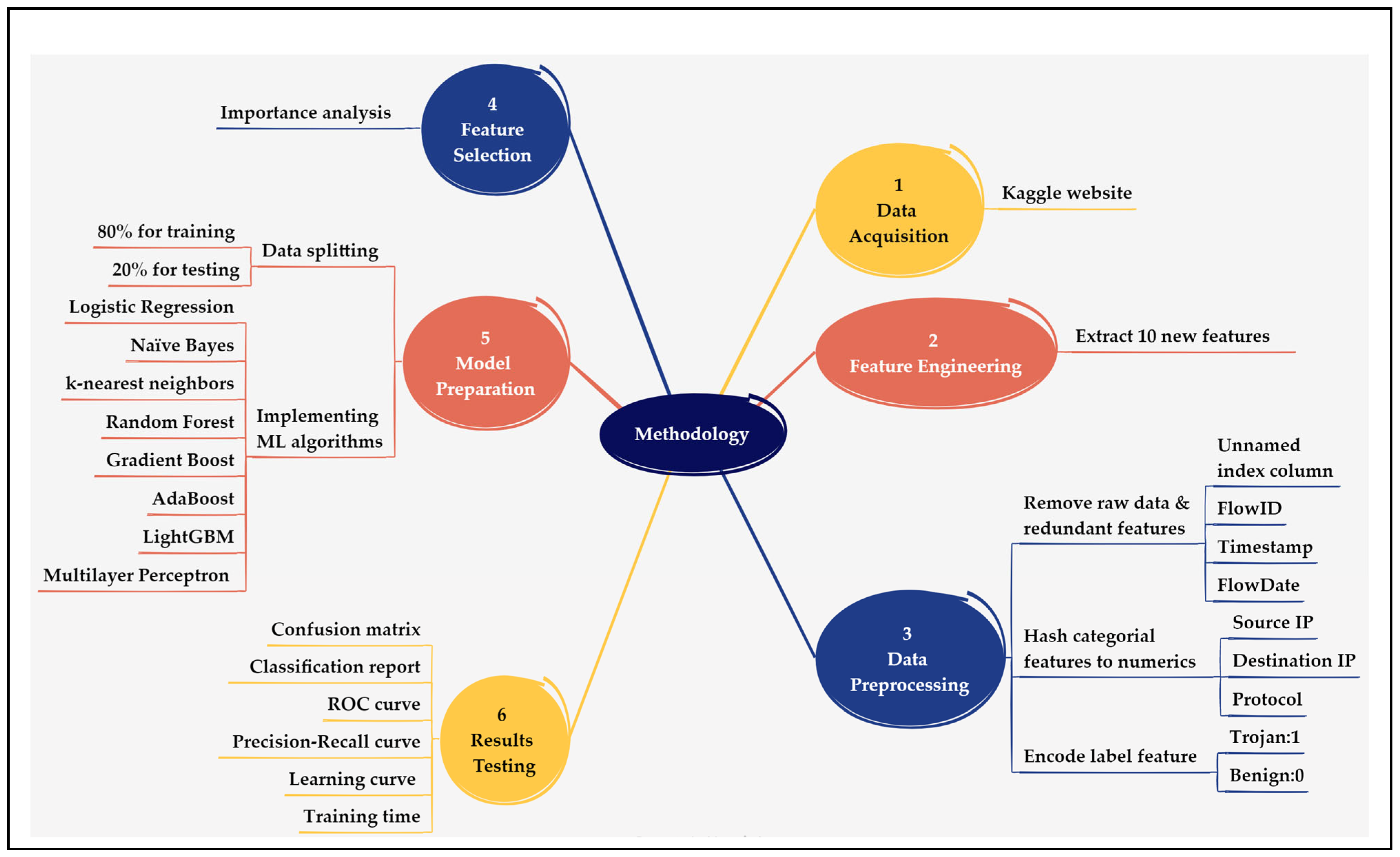
Figure 2. Research methodology workflow for RAT detection.
Ai 06 00237 g002
Figure 3. Distribution of RAT and benign samples in the dataset.
Ai 06 00237 g003
Figure 4. Feature engineering and selection roadmap for Model A and Model B.
Ai 06 00237 g004
Figure 5. Confusion matrix of Model A for RAT and benign classification.
Ai 06 00237 g005aAi 06 00237 g005b
Figure 6. ROC curves of Model A classifiers for distinguishing RAT and benign samples.
Ai 06 00237 g006
Figure 7. Precision–Recall curves of Model A classifiers for RAT and benign detection.
Ai 06 00237 g007
Figure 8. Learning curves and training time comparison of Model A classifiers.
Ai 06 00237 g008aAi 06 00237 g008b
Figure 9. Feature contribution in ensemble classifiers for Model A.
Ai 06 00237 g009
Table 1. Feature engineering results.
Source FeatureDerived Feature ClassificationDescription
TimestampFlowDateNetwork-based The calendar date of the flow. Used for grouping flows by day for aggregation.
HourNetwork-basedThe hour of the day when the flow occurred (0–23). Helps identify time-of-day attack patterns.
DayOfWeekNetwork-basedDay of the week (0 = Monday, 6 = Sunday). Used to detect weekday vs. weekend behavior variations.
SecondsSinceMidnightNetwork-basedTotal seconds elapsed since midnight. Provides more precise temporal behavior within a day.
Source IPSourceIP_FlowCountNetwork-behavioralTotal number of flows initiated by the source IP. Helps distinguish between active/inactive devices.
Source IP + TimestampTimeDiffFromLastFlowNetwork-behavioralTime difference (in seconds) between the current flow and the previous one from the same source IP. Indicates communication frequency.
Source IP + Destination IPUniqueDestinationsNetwork-behavioralNumber of unique destination IPs contacted by a source IP. A higher number may indicate scanning or RAT behavior.
Source IP + Destination IPUniqueSourcesNetwork-behavioralNumber of distinct source IPs contacting a destination. Can highlight unusual popularity.
Source IP +
Flow Duration
AvgFlowDurationNetwork-behavioralAverage flow duration per source IP. Helps characterize the typical length of communications from a source.
DayOfWeekIsWeekendNetwork-basedBinary value indicating whether the flow occurred on a weekend (1) or a weekday (0).
Table 2. Final model features description [27].
FeatureDescriptionImportance Score
1DayOfWeekDay of the week the flow was captured (0 = Monday, 6 = Sunday)0.247309
2SecondsSinceMidnightTime of the flow in seconds since midnight0.116366
3IsWeekendWhether the flow occurred during the weekend (1) or not (0)0.108793
4HourHour of the day when the flow occurred0.070363
5SourceIP_FlowCountNumber of flows originating from the same Source IP0.052595
6UniqueDestinationsNumber of distinct Destination IPs contacted by a Source IP0.047872
7Source IPIP address of the sender of the flow (hashed)0.043232
8AvgFlowDurationAverage duration of flows for a given Source IP0.038080
9UniqueSourcesNumber of unique Source IPs contacting a Destination IP0.018321
10Destination IPIP address of the receiver of the flow (hashed)0.013639
11Source PortPort number at the source device0.011500
12Flow DurationDuration of the flow in microseconds0.009645
13Flow IAT MinMinimum inter-arrival time between packets in the flow0.009489
14Flow IAT MaxMaximum inter-arrival time between packets in the flow0.009452
15Flow IAT MeanAverage inter-arrival time between packets in the flow0.009449
16Flow Packets/sRate of packets per second in the flow0.009331
17Fwd Packets/sRate of forward direction packets per second0.009276
18Init_Win_bytes_forwardInitial window size in bytes in the forward direction0.008862
19Destination PortPort number at the destination device0.007974
20Bwd Packets/sRate of backward direction packets per second0.006739
21Fwd IAT MaxMaximum inter-arrival time in the forward direction0.006585
22Fwd IAT TotalTotal inter-arrival time in the forward direction0.006416
23Init_Win_bytes_backwardInitial window size in bytes in the backward direction0.006255
24Fwd IAT MeanAverage inter-arrival time in the forward direction0.006102
25Fwd IAT MinMinimum inter-arrival time in the forward direction0.005927
26TimeDiffFromLastFlowTime since last flow from the same Source IP0.005879
27Flow Bytes/sRate of bytes per second in the flow0.004903
28Fwd IAT StdStandard deviation of inter-arrival time in forward direction0.004480
29Flow IAT StdStandard deviation of inter-arrival time in the flow0.003865
30Fwd Header LengthHeader length of packets in the forward direction0.003789
31Packet Length MeanAverage length of packets in the flow0.003656
32Fwd Packet Length MeanAverage packet length in forward direction0.003577
33Packet Length StdStandard deviation of packet lengths0.003453
34Fwd Header Length.1Duplicate of forward header length0.003444
35Avg Fwd Segment SizeAverage segment size in forward direction0.003373
36Average Packet SizeAverage size of packets in the flow0.003372
37Fwd Packet Length MaxMaximum packet length in forward direction0.003364
38Subflow Fwd BytesTotal bytes sent in subflow forward direction0.003334
39Total Length of Fwd PacketsSum of lengths of forward packets0.003305
40Packet Length VarianceVariance of packet lengths0.003305
41Bwd Packet Length MeanAverage packet length in backward direction0.003262
42Subflow Bwd BytesTotal bytes sent in subflow backward direction0.002940
43Bwd Header LengthHeader length of packets in the backward direction0.002908
44Avg Bwd Segment SizeAverage segment size in backward direction0.002906
45Total Length of Bwd PacketsSum of lengths of backward packets0.002833
46Bwd Packet Length MaxMaximum packet length in backward direction0.002690
47Bwd IAT MinMinimum inter-arrival time in backward direction0.002667
48Max Packet LengthMaximum packet length in the flow0.002644
49min_seg_size_forwardMinimum segment size in forward direction0.002493
50Bwd IAT TotalTotal inter-arrival time in backward direction0.002486
51Bwd IAT MaxMaximum inter-arrival time in backward direction0.002480
52Fwd Packet Length StdStandard deviation of packet lengths (forward)0.002471
53Bwd IAT MeanAverage inter-arrival time in backward direction0.002301
54Bwd IAT StdStandard deviation of inter-arrival times (backward)0.001968
55Bwd Packet Length StdStandard deviation of packet lengths (backward)0.001885
56Min Packet LengthMinimum packet length in the flow0.001853
57Bwd Packet Length MinMinimum packet length in backward direction0.001795
58Subflow Fwd PacketsNumber of packets sent in subflow forward0.001663
59Total Fwd PacketsTotal number of forward packets0.001584
60Total Backward PacketsTotal number of backward packets0.001560
61Fwd Packet Length MinMinimum packet length in forward direction0.001463
62Subflow Bwd PacketsNumber of packets sent in subflow backward0.001425
63Idle MeanAverage idle time between flows0.001324
64Idle MinMinimum idle time between flows0.001224
65Idle MaxMaximum idle time between flows0.001181
66Active MinMinimum active time between packets0.001162
67Active MeanAverage active time between packets0.001141
68Active MaxMaximum active time between packets0.001110
69URG Flag CountNumber of packets with the URG flag set0.001096
70ClassTarget label (0 = Benign, 1 = Trojan)1.000000
Table 3. Data splitting details for both models.
Class 0 (Benign)Class 1 (Trojan)Total SamplesClass Balance
Training Set69,43972,546141,985~49/51
Testing Set17,36018,13735,497~49/51
Balanced Training Set72,54672,546145,09250/50
Table 4. Classification report results of Model A: benign (0); Trojan (1).
AlgorithmPrecisionRecallF1-Score
Logistic Regression
(LR)
076%86%81%
185%74%79%
accuracy 80%
Naïve Bayes
(NB)
070%86%77%
183%64%72%
accuracy 75%
k-nearest neighbors
(KNN)
093%94%93%
194%93%94%
accuracy 94%
Random Forest
(RF)
099%98%98%
198%99%98%
accuracy 98%
Gradient Boosting
(GB)
0100%96%98%
196%100%98%
accuracy 98%
AdaBoost 097%96%97%
196%98%97%
accuracy 97%
LightGBM0100%94%97%
195%100%97%
accuracy 97%
Multilayer Perceptron
(MLP)
098%96%97%
196%98%97%
accuracy 97%
Table 5. Classification report results of Model B: benign (0); Trojan (1).
AlgorithmClassPrecisionRecallF1-Score
Logistic Regression
(LR)
049%51%50%
151%50%51%
accuracy 50%
Naïve Bayes
(NB)
050%87%64%
159%17%27%
accuracy 52%
k-nearest neighbors
(KNN)
053%53%53%
155%54%54%
accuracy 54%
Random Forest
(RF)
078%86%82%
185%77%81%
accuracy 81%
Gradient Boosting
(GB)
068%89%77%
186%60%70%
accuracy 74%
AdaBoost068%85%76%
181%62%70%
accuracy 73%
LightGBM070%90%79%
187%63%73%
accuracy 76%
Multilayer Perceptron
(MLP)
070%84%77%
181%66%73%
accuracy 75%
Table 6. Inference performance comparison of Model A classifiers: LR: logistic regression; NB: naïve Bayes; KNN: k-nearest neighbors; RF: random forest; GB: gradient boost; MLP: multilayer perceptron.
ClassifierAvg Latency
(MS/Sample)
Memory Usage (MB)CPU Utilization (%)
LR0.0006251616.863281201.6
NB0.0014551616.898438101.9
KNN1.9864211695.187500157.1
RF0.0154311690.18750097.1
GB0.0021771703.367188100.2
AdaBoost0.0110361703.36718896.2
LightGBM0.0023851645.976562180.3
MLP0.0020381703.417969380.6
Table 7. Related studies’ results. RF: random forest; KNN: k-nearest neighbors; NB: naïve Bayes; MLP: multilayer perceptron.
ReferenceYearClassifierAccuracy
[18]2016RF97.1%
KNN91.9%
NB43%
[34]2017RF95.2%
[35]2017RF99.7%
[20]2017NB96.5%
[22]2019RF99.5%
[36]2020KNN97.8%
[5]2020AdaBoost92%
[37]2022MLP95.8%
RF95.6%
[38]2022NB88.2%
RF100%
[21]2025RF74.8%
Disclaimer/Publisher’s Note: The statements, opinions and data contained in all publications are solely those of the individual author(s) and contributor(s) and not of MDPI and/or the editor(s). MDPI and/or the editor(s) disclaim responsibility for any injury to people or property resulting from any ideas, methods, instructions or products referred to in the content.